Emerging Communications for Wireless Sensor Networks Part 14 ppt
Bạn đang xem bản rút gọn của tài liệu. Xem và tải ngay bản đầy đủ của tài liệu tại đây (1.01 MB, 18 trang )
Indoor Location Tracking using Received Signal Strength Indicator 253
constraint, the individual device in wireless sensor network is normally limited in
processing capability, storage capacity, communication bandwidth, and battery power
supply (Culler, et al., 2004). The battery life-time and the communication bandwidth usage
are generally treated higher priority than the rest since in most applications, battery may not
be frequently recharged or replaced. Saving bandwidth or reducing the data transmission
among sensor nodes also means reducing power consumption used in communication.
Therefore, various algorithms such as collaborative signal processing, adaptive system,
distributed algorithm, and sensor fusion were developed for low power and bandwidth
applications.
Recently, a new trend of study is focused on in-network processing and intelligent system
such as (Tseng, et al., 2007) and (Yang, et al., 2007). For the applications of location tracking,
(Liu, et al., 2003) develop the initial concept of collaborative in-network processing for target
tracking. The focus is on vehicle tracking using acoustic and direction-of-arrival sensors.
(Lin, et al., 2004, 2006) presents in-network moving object tracking. The way of tracking
object is based on detection in a mass deployment of sensor nodes.
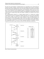
In general, the received RSSI values from reference nodes are sent to base station
immediately. The based station is an interface between WSN and computer, which collects
sufficient RSSI values and forwards them to the computer. In this case, location estimation
task is performed and stored in the computer.
Besides the monitoring of user’s activities, location information also can be used to support
the needs of network routing, data sensing, information query, self-organization, task
scheduling, field coverage, and etc. If the sensor nodes need the resultant location
information for decision making, the computer has to send the computed location
estimation result back to sensor nodes through the network. In this way, location estimation
does not consume processing power in the sensor nodes but this greatly increases the
wireless data transmission traffic for multi-user condition.
For a compromise, it is better to let the sensor nodes to collect all RSSI values and estimate
location coordinates locally within the WSN. The estimated location information is then
forwarded to a computer for monitoring or display. This approach also provides fast
location update rate due to short packets used. If the location information can be updated
immediately, the response and operation sensing tasks can be active, and the time taken for
decision making is short. The architectures of estimating location coordinate in a computer
and in sensor nodes are shown in Fig. 18.
Fig. 18. Two Scenarios of Location Estimation (Pu, 2009).
In Fig. 18(a), R1 to R3 are reference nodes in the area. A mobile node L1 is hold by a user
and moving around the area. L1 collects data from all reference nodes, and forwards them
to a computer. The packet includes the ID of each reference nodes (ID
R1
, ID
R2
, ID
R3
,), RSSI
values from each reference node (RSSI
1
, RSSI
2
, RSSI
3
,), and the ID of the mobile node (ID
L1
).
If the number of reference node increases, the packet size would be large. This largely
increases network traffic and load.
In Fig. 18 (b), R4 to R6 are reference nodes in the area. A mobile node L2 is hold by user and
moving around the area. L2 collects data from all reference nodes, and perform location
estimation locally. The resultant packet is then forwarded to computer. Hence, the packet
only includes the coordinate (x, y), space ID (SP
01
), and the ID of the mobile node (ID
L2
). If
the number of reference node increases, the packet size does not increase but still remains
small and constant because only the estimation result is forwarded to computer.
Wireless sensor network have substantial processing capability in the aggregate, but not
individually. For most of the low-power mobile device such as wireless sensor motes, the
processors or microcontrollers are limited in computational capability. For this reason,
indoor location estimation algorithms must be simple and ease of implementation.
For ensuring light-weight processing and tool-independent programming, it is necessary to
consider carefully that algorithms, mathematical calculations and processing are simple and
programmable to any low-power mobile devices which have limitation and constraints. The
main computational loads are in RSSI-distance conversion step and in trilateration step.
Computation using trilateration can be simplified by carefully planning the locations of
reference nodes at strategic locations and applying equations (21) to (23).
However, the computation of RSSI-distance conversion is not easy to be implemented in a
resource and computational power limited sensor node. This is because the computation of
exponential function is required in the equation (20), which generates large number if the
input data is not stable. To solve this problem, Taylor series can be used to avoid
exponential computation and simplify the calculation by selecting appropriate length of
expression L as shown in the following expression (Pu, 2009):
L
i
iL
i
x
d
L
xxxx
dd
1
0
321
0
!
1
!
!3!2!1
1
(27)
where
n
PP
x
drdr
10
10ln
)(0
(28)
4. Conclusions
This chapter is to provide essential knowledge on the development of a location awareness
system for location monitoring in ubiquitous applications. The location system must be able
to estimate fine-grained location in indoor environment. Wireless sensor network was
selected as the main body of the system. All data from wireless sensor network are sent to a
base station for centralized operation and management.
Emerging Communications for Wireless Sensor Networks254
Based on the way of ranging, location system can be time measurement or signal
measurement. Time measurement can be achieved using the combination of RF and
ultrasound for time difference of arrival (TDOA). Signal measurement can be achieved by
converting received signal strength indicator (RSSI) to distance. Since RSSI does not need
additional dedicated devices for ranging, and the power consumption is much lower than
other distance measurement methods, it was selected as the ranging method in this research.
With the existing technology, RSSI ranging is still not a perfect solution for fine-grained
location tracking because of inaccurate and uncertain input data when it is used in indoor
environment. Therefore, it is required to be improved through research studies. Three
important processes of indoor location tracking can be studied to improve the performance.
First, the signal quality of RSSI in indoor environment must be studied for accuracy and
precision improvement. Second, the methods used for environmental characterization need
to be re-investigated so that a convenient and effective calibration method or procedure can
be developed to obtained accurate environmental parameters. Third, the positioning
algorithm must be reconsidered to exploit an innovative way of location estimation that
may provide advantages additional to traditional positioning algorithm.
5. References
Abdalla, M.; Feeney, S. M. & Salous, S. (2003). Antenna Array and Quadrature Calibration
for Angle of Arrival Estimation, SCI, Florida, July 2003.
Bulusu, N.; Heidemann, J. & Estrin, D. (2000). GPS-less Low Cost Outdoor Localization for
Very Small Devices, IEEE Personal Communications Magazine, vol.7, no.5, pp.28–34.
Cong, T X.; Kim, E. & Koo, I. (2008). An Efficient RSS-Based Localization Scheme with
Calibration in Wireless Sensor Networks, IEICE Trans. Communications, vol.E91-B,
no.12, pp.4013–4016.
Culler, D.; Estrin, D. & Srivastava, M. (2004). Guest Editors’s Introduction: Overview of
Sensor Networks, IEEE Computer Society, vol. 37, no. 8, pp.4149.
Eltahir, I. K. (2007). The Impact of Different Radio Propagation Models for Mobile Ad hoc
NETworks (MANET) in Urban Area Environment, AusWireless, pp. 3038,
Sydney, Australia, Aug 2007.
Favre-Bulle, B.; Prenninger, J. & Eitzinger, C. (1998). Efficient Tracking of 3D-Robot
Positions by Dynamic Triangulation, MTC, pp.446–449, St. Paul, Minnesota, May
1998.
He, J. (2008). Optimizing 2-D Triangulations by the Steepest Descent Method, PACIIA,
pp.939–943, Wuhan, China, December 2008.
He, T.; Huang, C.; Blum, B. M.; Stankovic, J. A. & Abdelzaher, T. F. (2005). Range-Free
Localization and Its Impact on Large Scale Sensor Networks, ACM Trans. Embedded
Computing Systems, vol.4, no.4, November 2005, pp.877–906.
Hightower, J. & Borriello, G. (2001). Location Systems for Ubiquitous Computing, IEEE
Computer, vol.34, no.8, August 2001, pp.57–66.
Kamath, S.; Meisner, E. & Isler, V. (2007). Triangulation Based Multi Target Tracking with
Mobile Sensor Networks, ICRA, pp.3283–3288, Roma, Italy, April 2007.
Li, X Y.; Calinescu, G.; Wan, P J. & Wang, Y. (2003). Localized Delaunay Triangulation with
Application in Ad Hoc Wireless Networks, IEEE Trans. Parallel and Distributed
Systems, vol.14, no.10, pp.1035–1047.
Li, X Y.; Wang, Y. & Frieder, O. (2003). Localized Routing for Wireless Ad Hoc Networks,
ICC, pp.443–447, Anchorage, Alaska, USA, May 2003.
Lin C Y. & Tseng, Y C. (2004). Structures for In-Network Moving Object Tracking in
Wireless Sensor Networks, BROADNET, pp.718727, San Jose, California, USA,
2004.
Lin, C Y.; Peng, W C. & Tseng, Y C. (2006). Efficient In-network Moving Object Tracking
in Wireless Sensor Network, IEEE Transactions on Mobile Computing, vol.5, no.8,
pp.10441056.
Liu, J.; Reich, J. & Zhao, F. (2003). Collaborative In-Network Processing for Target Tracking,
EURASIP Journal on Applied Signal Processing, vol.4, pp.378391.
Mak, L. C & Furukawa, T. (2006). A ToA-based Approach to NLOS Localization Usiong
Low-Frequency Sound, ACRA, Auckland, New Zealand, December 2006.
Najar, M. & Vidal, J. (2001). Kalman Tracking based on TDOA for UMTS Mobile Location,
PIMRC, pp.B45–B49, San Diego, California, USA, September 2001.
Nakajima, N. (2007). Indoor Wireless Network for Person Location Identification and Vital
Data Collection, ISMICT, Oulu, Finland, December 2007.
Niculescu, D. & Nath, B. (2003). DV Based Positioning in Ad hoc Networks. Journal of
Telecommunication Systems, vol.22, no.1-4, pp.1018–4864.
Phaiboon, S. (2002). An Empirically Based Path Loss Model for Indoor Wireless Channels in
Laboratory Building, IEEE TENCON, pp.10201023, vol.2, October 2002.
Pu, C C. (2009). Development of a New Collaborative Ranging Algorithm for RSSI Indoor Location
Tracking in WSN, PhD Thesis, Dongseo University, South Korea.
Rao, S.V.; Xu, X. & Sahni, S. (2007). A Computational Geometry Method for DTOA
Triangulation, ICIF, pp.1–7, Quebec, Canada, July 2007.
Rice, A & Harle, R. (2005). Evaluating Lateration-based Positioning Algorithms for Fine-
grained Tracking, DIALM-POMC, pp.54–61, Cologne, Germany, September 2005.
Satyanarayana, D. & Rao, S. V. (2008). Local Delaunay Triangulation for Mobile Nodes,
ICETET, pp.282–287, Nagpur, Maharashtra, India, July 2008.
Savvides, A.; Han, C C. & Mani, B. (2001). Strivastava. Dynamic Fine-Grained Localization
in Ad-Hoc Networks of Sensors, MobiCom, pp.166–179, Rome, Italy, July 2001.
Sklar, B. (1997). Rayleigh Fading Channels in Mobile Digital Communication Systems:
Characterization and Mitigation, IEEE Communications Magazine, vol. 35, no. 7, pp.
90109.
Smith, A.; Balakrishnan, H.; Goraczko, M. & Priyantha, N. (2004). Tracking Moving Devices
with the Cricket Location System, MobiSYS, pp.190–202, Boston, USA.
Thomas, F. & Ros, L. (2005). Revisiting Trilateration for Robot Localization, IEEE Robotics,
vol.21, no.1, pp.93101.
Tian, H.; Wang, S. & Xie, H. (2007). Localization using Cooperative AOA Approach,
WiCOM, pp.2416–2419, Shanghai, China, September 2007.
Tseng, Y C; Chen, C C.; Lee, C. & Huang, Y K. (2007). Incremental In-Network RNN
Search in Wireless Sensor Networks, ICPPW, pp.6464, XiAn, China, September
2007.
Yang, H Y.; Peng, W C. & Lo, C H. (2007). Optimizing Multiple In-Network Aggregate
Queries in Wireless Sensor Networks, LNCS, vol.4443, pp.870875.
Indoor Location Tracking using Received Signal Strength Indicator 255
Based on the way of ranging, location system can be time measurement or signal
measurement. Time measurement can be achieved using the combination of RF and
ultrasound for time difference of arrival (TDOA). Signal measurement can be achieved by
converting received signal strength indicator (RSSI) to distance. Since RSSI does not need
additional dedicated devices for ranging, and the power consumption is much lower than
other distance measurement methods, it was selected as the ranging method in this research.
With the existing technology, RSSI ranging is still not a perfect solution for fine-grained
location tracking because of inaccurate and uncertain input data when it is used in indoor
environment. Therefore, it is required to be improved through research studies. Three
important processes of indoor location tracking can be studied to improve the performance.
First, the signal quality of RSSI in indoor environment must be studied for accuracy and
precision improvement. Second, the methods used for environmental characterization need
to be re-investigated so that a convenient and effective calibration method or procedure can
be developed to obtained accurate environmental parameters. Third, the positioning
algorithm must be reconsidered to exploit an innovative way of location estimation that
may provide advantages additional to traditional positioning algorithm.
5. References
Abdalla, M.; Feeney, S. M. & Salous, S. (2003). Antenna Array and Quadrature Calibration
for Angle of Arrival Estimation, SCI, Florida, July 2003.
Bulusu, N.; Heidemann, J. & Estrin, D. (2000). GPS-less Low Cost Outdoor Localization for
Very Small Devices, IEEE Personal Communications Magazine, vol.7, no.5, pp.28–34.
Cong, T X.; Kim, E. & Koo, I. (2008). An Efficient RSS-Based Localization Scheme with
Calibration in Wireless Sensor Networks, IEICE Trans. Communications, vol.E91-B,
no.12, pp.4013–4016.
Culler, D.; Estrin, D. & Srivastava, M. (2004). Guest Editors’s Introduction: Overview of
Sensor Networks, IEEE Computer Society, vol. 37, no. 8, pp.4149.
Eltahir, I. K. (2007). The Impact of Different Radio Propagation Models for Mobile Ad hoc
NETworks (MANET) in Urban Area Environment, AusWireless, pp. 3038,
Sydney, Australia, Aug 2007.
Favre-Bulle, B.; Prenninger, J. & Eitzinger, C. (1998). Efficient Tracking of 3D-Robot
Positions by Dynamic Triangulation, MTC, pp.446–449, St. Paul, Minnesota, May
1998.
He, J. (2008). Optimizing 2-D Triangulations by the Steepest Descent Method, PACIIA,
pp.939–943, Wuhan, China, December 2008.
He, T.; Huang, C.; Blum, B. M.; Stankovic, J. A. & Abdelzaher, T. F. (2005). Range-Free
Localization and Its Impact on Large Scale Sensor Networks, ACM Trans. Embedded
Computing Systems, vol.4, no.4, November 2005, pp.877–906.
Hightower, J. & Borriello, G. (2001). Location Systems for Ubiquitous Computing, IEEE
Computer, vol.34, no.8, August 2001, pp.57–66.
Kamath, S.; Meisner, E. & Isler, V. (2007). Triangulation Based Multi Target Tracking with
Mobile Sensor Networks, ICRA, pp.3283–3288, Roma, Italy, April 2007.
Li, X Y.; Calinescu, G.; Wan, P J. & Wang, Y. (2003). Localized Delaunay Triangulation with
Application in Ad Hoc Wireless Networks, IEEE Trans. Parallel and Distributed
Systems, vol.14, no.10, pp.1035–1047.
Li, X Y.; Wang, Y. & Frieder, O. (2003). Localized Routing for Wireless Ad Hoc Networks,
ICC, pp.443–447, Anchorage, Alaska, USA, May 2003.
Lin C Y. & Tseng, Y C. (2004). Structures for In-Network Moving Object Tracking in
Wireless Sensor Networks, BROADNET, pp.718727, San Jose, California, USA,
2004.
Lin, C Y.; Peng, W C. & Tseng, Y C. (2006). Efficient In-network Moving Object Tracking
in Wireless Sensor Network, IEEE Transactions on Mobile Computing, vol.5, no.8,
pp.10441056.
Liu, J.; Reich, J. & Zhao, F. (2003). Collaborative In-Network Processing for Target Tracking,
EURASIP Journal on Applied Signal Processing, vol.4, pp.378391.
Mak, L. C & Furukawa, T. (2006). A ToA-based Approach to NLOS Localization Usiong
Low-Frequency Sound, ACRA, Auckland, New Zealand, December 2006.
Najar, M. & Vidal, J. (2001). Kalman Tracking based on TDOA for UMTS Mobile Location,
PIMRC, pp.B45–B49, San Diego, California, USA, September 2001.
Nakajima, N. (2007). Indoor Wireless Network for Person Location Identification and Vital
Data Collection, ISMICT, Oulu, Finland, December 2007.
Niculescu, D. & Nath, B. (2003). DV Based Positioning in Ad hoc Networks. Journal of
Telecommunication Systems, vol.22, no.1-4, pp.1018–4864.
Phaiboon, S. (2002). An Empirically Based Path Loss Model for Indoor Wireless Channels in
Laboratory Building, IEEE TENCON, pp.10201023, vol.2, October 2002.
Pu, C C. (2009). Development of a New Collaborative Ranging Algorithm for RSSI Indoor Location
Tracking in WSN, PhD Thesis, Dongseo University, South Korea.
Rao, S.V.; Xu, X. & Sahni, S. (2007). A Computational Geometry Method for DTOA
Triangulation, ICIF, pp.1–7, Quebec, Canada, July 2007.
Rice, A & Harle, R. (2005). Evaluating Lateration-based Positioning Algorithms for Fine-
grained Tracking, DIALM-POMC, pp.54–61, Cologne, Germany, September 2005.
Satyanarayana, D. & Rao, S. V. (2008). Local Delaunay Triangulation for Mobile Nodes,
ICETET, pp.282–287, Nagpur, Maharashtra, India, July 2008.
Savvides, A.; Han, C C. & Mani, B. (2001). Strivastava. Dynamic Fine-Grained Localization
in Ad-Hoc Networks of Sensors, MobiCom, pp.166–179, Rome, Italy, July 2001.
Sklar, B. (1997). Rayleigh Fading Channels in Mobile Digital Communication Systems:
Characterization and Mitigation, IEEE Communications Magazine, vol. 35, no. 7, pp.
90109.
Smith, A.; Balakrishnan, H.; Goraczko, M. & Priyantha, N. (2004). Tracking Moving Devices
with the Cricket Location System, MobiSYS, pp.190–202, Boston, USA.
Thomas, F. & Ros, L. (2005). Revisiting Trilateration for Robot Localization, IEEE Robotics,
vol.21, no.1, pp.93101.
Tian, H.; Wang, S. & Xie, H. (2007). Localization using Cooperative AOA Approach,
WiCOM, pp.2416–2419, Shanghai, China, September 2007.
Tseng, Y C; Chen, C C.; Lee, C. & Huang, Y K. (2007). Incremental In-Network RNN
Search in Wireless Sensor Networks, ICPPW, pp.6464, XiAn, China, September
2007.
Yang, H Y.; Peng, W C. & Lo, C H. (2007). Optimizing Multiple In-Network Aggregate
Queries in Wireless Sensor Networks, LNCS, vol.4443, pp.870875.
Emerging Communications for Wireless Sensor Networks256
Zhao, F.; Liu, J.; Liu, J.; Guibas, L. & Reich, J. (2003). Collaborative signal and information
processing: an information directed approach, Proc. IEEE, vol.91, no.8, pp.1199–
1209.
Zhao, F. & Guibas, L. J. (2004). Wireless Sensor Networks: An Information Processing Approach,
Elsevier: Morgan Kaufmann Series.
Mobile Location Tracking Scheme for Wireless
Sensor Networks with Decient Number of Sensor Nodes 257
Mobile Location Tracking Scheme for Wireless Sensor Networks with
Decient Number of Sensor Nodes
Po-Hsuan Tseng, Wen-Jiunn Liu and Kai-Ten Feng
X
Mobile Location Tracking Scheme
for Wireless Sensor Networks with
Deficient Number of Sensor Nodes
Po-Hsuan Tseng, Wen-Jiunn Liu and Kai-Ten Feng
Department of Communication Engineering, National Chiao Tung University
Taiwan, R.O.C.
1.Introduction
A wireless sensor network (WSN) consists of sensor nodes (SNs) with wireless
communication capabilities for specific sensing tasks. Among different applications,
wireless location technologies which are designated to estimate the position of SNs
(Geziciet al., 2005) (Haraet al., 2005) (Patwari et al., 2005)have drawn a lot of attention
over the past few decades. There are increasing demands for commercial applications to
adopt location tracking information within their system design, such as navigation
systems, location-based billing, health care systems, and intelligent transportation
systems. With emergent interests in location-based services (Perusco & Michael, 2007),
location estimation and tracking algorithms with enhanced precision become necessitate
for the applications under different circumstances.
The location estimation schemes have been widely proposed and employed in the
wireless communication system. These schemes locate the position of a mobile sensor (MS)
based on the measured radio signals from its neighborhood anchor nodes (ANs). The
representative algorithms for the measured distance techniques are the Time-Of-Arrival
(TOA),the Time Difference-Of-Arrival (TDOA), and the Angle-Of-Arrival (AOA). The
TOA scheme measures the arrival time of the radio signals coming from different wireless
BSs; while the TDOA scheme measures the time difference between the radio signals. The
AOA technique is conducted within the BS by observing the arriving angle of the signals
coming from the MS.
It is recognized that the equations associated with the location estimation schemes are
inherently nonlinear. The uncertainties induced by the measurement noises make it more
difficult to acquire the estimated MS position with tolerable precision. The Taylor Series
Expansion (TSE) method was utilized in(Foy, 1976) to acquire the location estimation of
the MS from the TOA measurements. The method requires iterative processes to obtain
the location estimate from a linearized system. The major drawback of the TSE scheme is
that it may suffer from the convergence problem due to an incorrect initial guess of the
MS’s position. The two-step Least Square (LS) method was adopted to solve the location
estimation problem from the TOA (Wanget al., 2003), the TDOA (Chen& Ho, 1994), and
the hybrid TOA/TDOA(Tseng & Feng, 2009) measurements. It is an approximate
12
Emerging Communications for Wireless Sensor Networks258
realization of the Maximum Likelihood (ML) estimator and does not require iterative
processes. The two-step LS scheme is advantageous in its computational efficiency with
adequate accuracy for location estimation.
In addition to the estimation of a MS’s position, trajectory tracking of a moving MS has
been studied. The Extended Kalman Filter (EKF) scheme is considered the well-adopted
method for location tracking. The EKF algorithm estimates the MS’s position, speed, and
acceleration via the linearization of measurement inputs. The Kalman Tracking (KT)
scheme (Nájar& Vidal,2001) distinguishes the linear part from the originally nonlinear
equations for location estimation. The linear aspect is exploited within the Kalman
filtering formulation; while the nonlinear term is served as an external measurement
input to the Kalman filter. The Cascade Location Tracking(CLT) scheme (Chen &Feng,
2005) utilizes the two-step LS method for initial location estimation of the MS.The Kalman
filtering technique is employed to smooth out and to trace the position of the MS based on
its previously estimated data.
With the characteristics of simplicity and high accuracy, the range-based positioning
method based on triangulation approach is considered according to the time-of-arrival
measurements. The location of a MS can be estimated and traced from the availability of
enough SNs with known positions, denoted as anchor nodes ANs. In general, at least
three ANs are required to perform two-dimensional location estimation for an MS.
However, enough signal sources for location estimation and tracking may not always
happen under the WSN scenarios. Unlike the regular deployment of satellites or cellular
base stations, the ANs within the WSN are in general spontaneously and arbitrarily
deployed. Even though there can be high density of SNs within certain area, the number
of ANs with known position can still be limited. Moreover, the transmission ranges for
SNs are comparably shorter than both the satellite-based (Kuusniemi et al., 2007) and the
cellular-based (Zhao, 2002) systems. Therefore, there is high probability for the node
deficiency problem (i.e., the number of available ANs is less than three) to occur within
the WSN, especially under the situations that the SNs are moving. Due to the deficiency of
signal sources, most of the existing location estimation and tracking schemes becomes
inapplicable for the WSNs.
In this book chapter, a predictive location tracking (PLT) algorithm is proposed to
alleviate the problem with insufficient measurement inputs for the WSNs. Location
tracking can still be performed even with only two ANs or a single AN available to be
exploited. The predictive information obtained from the Kalman filtering technique (Zaidi
& Mark, 2005) is adopted as the virtual signal sources, which are incorporated into the
two-step least square method for location estimation and tracking. Persistent accuracy for
location tracking can be achieved by adopting the proposed PLT scheme, especially under
the situations with inadequate signal sources. Numerical results demonstrate that the
proposed PLT algorithm can achieve better precision in comparison with other location
tracking schemes under the WSNs.
2. Preliminaries
2.1 Mathematical Modeling
In order to facilitate the design of the proposed PLT algorithm, the signal model for the TOA
measurements is utilized. The set r
k
contains all the available measured relative distance at
the k
th
time step, i.e., r
k
= { r
1,k
, r
2,k
, …, r
i,k
, …,
}, where
denotes the number of
available ANs. The measured relative distance (r
i,k
) between the MS and the i
th
AN(obtained
at the k
th
time step) can be represented as
r
i,k
= c· t
i,k
=
i,k
+ n
i,k
+ e
i,k
(1)
Where t
i,k
denotes the TOA measurement obtained from the i
th
AN at the k
th
time step, and c
is the speed of light. r
i,k
is contaminated with the TOA measurement noise n
i,k
and the NLOS
error e
i,k
. It is noted that the measurement noise n
i,k
is in general considered as zero mean
with Gaussian distribution. On the other hand, the NLOS error e
i,k
is modeled as
exponentially-distributed for representing the positive bias due to the NLOS effect (Lee,
1993). The noiseless relative distance ζ
i,k
in (1) between the MS’s true position and the i
th
AN
can be obtained as
ζ
i,k
= [ (x
k
- x
i,k
)
2
+ (y
k
- y
i,k
)
2
]
1/2
(2)
where x
k
= [x
k
y
k
] represents the MS’s true position and x
i,k
= [x
i,k
y
i,k
] is the location of the
i
th
AN for i = 1 to
. Therefore, the set of all the available ANs at the k
th
time step can be
obtained as P
AN,k
= { x
1,k
, x
2,k
, …,x
i,k
, …,
}.
2.2Two-Step LS Estimator
The two-step LS scheme (Chen& Ho, 1994) is utilized as the baseline location estimator for
the proposed predictive location tracking algorithms. It is noticed that three TOA
measurements are required for the two-step LS method in order to solve for the location
estimation problem. The concept of the two-step LS scheme is to acquire an intermediate
location estimate in the first step with the definition of a new variable β
k
, which is
mathematically related to the MS’s position, i.e., β
k
= x
k
2
+ y
k
2
. At this stage, the variable β
k
is
assumed to be uncorrelated to the MS’s position. This assumption effectively transforms the
nonlinear equations for location estimation into a set of linear equations, which can be
directly solved by the LS method. Moreover, the elements within the associated covariance
matrix are selected based on the standard deviation from the measurements. The variations
within the corresponding signal paths are therefore considered within the problem
formulation.
The second step of the method primarily considers the relationship that the variable β
k
is
equal to x
k
2
+ y
k
2
, which was originally assumed to be uncorrelated in the first step.
Improved location estimation can be obtained after the adjustment from the second step.
The detail algorithm of the two-step LS method for location estimation can be found in
(Chen& Ho, 1994) (Cong & Zhuang, 2002) (Wang et al., 2003).
Mobile Location Tracking Scheme for Wireless
Sensor Networks with Decient Number of Sensor Nodes 259
realization of the Maximum Likelihood (ML) estimator and does not require iterative
processes. The two-step LS scheme is advantageous in its computational efficiency with
adequate accuracy for location estimation.
In addition to the estimation of a MS’s position, trajectory tracking of a moving MS has
been studied. The Extended Kalman Filter (EKF) scheme is considered the well-adopted
method for location tracking. The EKF algorithm estimates the MS’s position, speed, and
acceleration via the linearization of measurement inputs. The Kalman Tracking (KT)
scheme (Nájar& Vidal,2001) distinguishes the linear part from the originally nonlinear
equations for location estimation. The linear aspect is exploited within the Kalman
filtering formulation; while the nonlinear term is served as an external measurement
input to the Kalman filter. The Cascade Location Tracking(CLT) scheme (Chen &Feng,
2005) utilizes the two-step LS method for initial location estimation of the MS.The Kalman
filtering technique is employed to smooth out and to trace the position of the MS based on
its previously estimated data.
With the characteristics of simplicity and high accuracy, the range-based positioning
method based on triangulation approach is considered according to the time-of-arrival
measurements. The location of a MS can be estimated and traced from the availability of
enough SNs with known positions, denoted as anchor nodes ANs. In general, at least
three ANs are required to perform two-dimensional location estimation for an MS.
However, enough signal sources for location estimation and tracking may not always
happen under the WSN scenarios. Unlike the regular deployment of satellites or cellular
base stations, the ANs within the WSN are in general spontaneously and arbitrarily
deployed. Even though there can be high density of SNs within certain area, the number
of ANs with known position can still be limited. Moreover, the transmission ranges for
SNs are comparably shorter than both the satellite-based (Kuusniemi et al., 2007) and the
cellular-based (Zhao, 2002) systems. Therefore, there is high probability for the node
deficiency problem (i.e., the number of available ANs is less than three) to occur within
the WSN, especially under the situations that the SNs are moving. Due to the deficiency of
signal sources, most of the existing location estimation and tracking schemes becomes
inapplicable for the WSNs.
In this book chapter, a predictive location tracking (PLT) algorithm is proposed to
alleviate the problem with insufficient measurement inputs for the WSNs. Location
tracking can still be performed even with only two ANs or a single AN available to be
exploited. The predictive information obtained from the Kalman filtering technique (Zaidi
& Mark, 2005) is adopted as the virtual signal sources, which are incorporated into the
two-step least square method for location estimation and tracking. Persistent accuracy for
location tracking can be achieved by adopting the proposed PLT scheme, especially under
the situations with inadequate signal sources. Numerical results demonstrate that the
proposed PLT algorithm can achieve better precision in comparison with other location
tracking schemes under the WSNs.
2. Preliminaries
2.1 Mathematical Modeling
In order to facilitate the design of the proposed PLT algorithm, the signal model for the TOA
measurements is utilized. The set r
k
contains all the available measured relative distance at
the k
th
time step, i.e., r
k
= { r
1,k
, r
2,k
, …, r
i,k
, …,
}, where
denotes the number of
available ANs. The measured relative distance (r
i,k
) between the MS and the i
th
AN(obtained
at the k
th
time step) can be represented as
r
i,k
= c· t
i,k
=
i,k
+ n
i,k
+ e
i,k
(1)
Where t
i,k
denotes the TOA measurement obtained from the i
th
AN at the k
th
time step, and c
is the speed of light. r
i,k
is contaminated with the TOA measurement noise n
i,k
and the NLOS
error e
i,k
. It is noted that the measurement noise n
i,k
is in general considered as zero mean
with Gaussian distribution. On the other hand, the NLOS error e
i,k
is modeled as
exponentially-distributed for representing the positive bias due to the NLOS effect (Lee,
1993). The noiseless relative distance ζ
i,k
in (1) between the MS’s true position and the i
th
AN
can be obtained as
ζ
i,k
= [ (x
k
- x
i,k
)
2
+ (y
k
- y
i,k
)
2
]
1/2
(2)
where x
k
= [x
k
y
k
] represents the MS’s true position and x
i,k
= [x
i,k
y
i,k
] is the location of the
i
th
AN for i = 1 to
. Therefore, the set of all the available ANs at the k
th
time step can be
obtained as P
AN,k
= { x
1,k
, x
2,k
, …,x
i,k
, …,
}.
2.2Two-Step LS Estimator
The two-step LS scheme (Chen& Ho, 1994) is utilized as the baseline location estimator for
the proposed predictive location tracking algorithms. It is noticed that three TOA
measurements are required for the two-step LS method in order to solve for the location
estimation problem. The concept of the two-step LS scheme is to acquire an intermediate
location estimate in the first step with the definition of a new variable β
k
, which is
mathematically related to the MS’s position, i.e., β
k
= x
k
2
+ y
k
2
. At this stage, the variable β
k
is
assumed to be uncorrelated to the MS’s position. This assumption effectively transforms the
nonlinear equations for location estimation into a set of linear equations, which can be
directly solved by the LS method. Moreover, the elements within the associated covariance
matrix are selected based on the standard deviation from the measurements. The variations
within the corresponding signal paths are therefore considered within the problem
formulation.
The second step of the method primarily considers the relationship that the variable β
k
is
equal to x
k
2
+ y
k
2
, which was originally assumed to be uncorrelated in the first step.
Improved location estimation can be obtained after the adjustment from the second step.
The detail algorithm of the two-step LS method for location estimation can be found in
(Chen& Ho, 1994) (Cong & Zhuang, 2002) (Wang et al., 2003).
Emerging Communications for Wireless Sensor Networks260
3. Architecture overview of proposed PLT algorithm
Fig. 1.The architecture diagrams of (a) the KT scheme; (b) the CLTscheme; and (c) the
proposed PLT scheme.
The objective of the proposed PLT algorithm is to utilize the predictive information acquired
from the Kalman filter to serve as the assisted measurement inputs while the environments
are deficient with signal sources. Fig. 1 illustrates the system architectures of the KT(Njar&
Vidal,2001), the CLT (Chen & Feng, 2005) and the proposed PLT scheme. The TOA signals
(r
k
as in (1)) associated with the corresponding location set of the ANs (P
AN,k
) are obtained as
the signal inputs to each of the system, which result in the estimated state vector of the MS,
i.e.
where
represents the MS’s estimated position,
is the estimated velocity, and
= denotes the estimated acceleration.
Since the equations (i.e., (1) and (2)) associated with the location estimation are intrinsically
nonlinear, different mechanisms are considered within the existing algorithms for location
tracking. The KT scheme (as shown in Fig. 1.(a)) explores the linear aspect of location
estimation within the Kalman filtering formulation; while the nonlinear term (i.e.,
) is treated as an additional measurement input to the Kalman filter. It is stated within the
KT scheme that the value of the nonlinear term can be obtained from an external location
estimator, e.g. via the two-step LS method. Consequently, the estimation accuracy of the KT
algorithm greatly depends on the precision of the additional location estimator. On the other
hand, the CLT scheme (as illustrated in Fig. 1.(b)) adopts the two-step LS method to acquire
the preliminary location estimate of the MS. The Kalman Filter is utilized to smooth out the
estimation error by tracing the estimated state vector
of the MS.
The architecture of the proposed PLT scheme is illustrated in Fig. 1.(c). It can be seen that
the PLT algorithm will be thesame as the CLT scheme while
≥3, i.e. the number of
available ANs is greater than or equal to three. However, the effectiveness of the PLT
schemes is revealed as1≤
<3, i.e. with deficient measurement inputs. The predictive state
information obtained from the Kalman filter is utilized for acquiring the assisted
information, which will be fed back into the location estimator. The extended sets for the
locations of the ANs (i.e.,
) and the measured relative
distances(i.e.,
) will be utilized as the inputs to thelocation estimator. The sets
of the virtual ANs’ locations
and the virtual measurements
are defined asfollows.
Definition 1 (Virtual Anchor Nodes).Within the PLT formulation, the virtual Anchor
Nodes are considered as the designed locations for assisting the location tracking of the MS
under the environments with deficient signal sources. The set of virtual ANs
is
defined under two different numbers of
as
(3)
Definition 2 (Virtual Measurements).Within thePLT formulation, the virtual measurements
are utilized to provide assisted measurement inputs while the signal sources are insufficient.
Associating with the designed set of virtual ANs
, the corresponding set of virtual
measurements is defined as
(4)
It is noticed that the major task of the PLT scheme is to design and to acquire the values of
and
for the two cases (i.e.
= 1 and2) with inadequate signal sources. In both the
KT andthe CLT schemes, the estimated state vector
can onlybe updated by the internal
prediction mechanism of the Kalman filter while there are insufficient numbers of ANs
(i.e.,
<3 as shown in Fig. 1.(a) and 1.(b) with the dashed lines). The location estimator (i.e.,
the two-step LS method) is consequently disabled owing to the inadequate number of the
signal sources. The tracking capabilities of both schemes significantly depend on the
correctness of the Kalman filter’s prediction mechanism. Therefore, the performance for
location tracking can be severely degraded due to the changing behavior of the MS, i.e., with
the variations from the MS’s acceleration.
On the other hand, the proposed PLT algorithm can still provide satisfactory tracking
performance with deficient measurement inputs, i.e., with
= 1 and 2. Under these
circumstances, the locationestimator is still effective with the additional virtual ANs
and the virtual measurements
, whichare imposed from the predictive output of the
Kalman filter (as shown in Fig. 1.(c)). It is also noted that the PLT scheme will perform the
same as the CLT method under the case with no signal input, i.e., under
= 0. The virtual
ANs’ location set
andthe virtual measurements
by exploiting the PLTformulation
are presented in the next section.
Mobile Location Tracking Scheme for Wireless
Sensor Networks with Decient Number of Sensor Nodes 261
3. Architecture overview of proposed PLT algorithm
Fig. 1.The architecture diagrams of (a) the KT scheme; (b) the CLTscheme; and (c) the
proposed PLT scheme.
The objective of the proposed PLT algorithm is to utilize the predictive information acquired
from the Kalman filter to serve as the assisted measurement inputs while the environments
are deficient with signal sources. Fig. 1 illustrates the system architectures of the KT(Njar&
Vidal,2001), the CLT (Chen & Feng, 2005) and the proposed PLT scheme. The TOA signals
(r
k
as in (1)) associated with the corresponding location set of the ANs (P
AN,k
) are obtained as
the signal inputs to each of the system, which result in the estimated state vector of the MS,
i.e.
where
represents the MS’s estimated position,
is the estimated velocity, and
= denotes the estimated acceleration.
Since the equations (i.e., (1) and (2)) associated with the location estimation are intrinsically
nonlinear, different mechanisms are considered within the existing algorithms for location
tracking. The KT scheme (as shown in Fig. 1.(a)) explores the linear aspect of location
estimation within the Kalman filtering formulation; while the nonlinear term (i.e.,
) is treated as an additional measurement input to the Kalman filter. It is stated within the
KT scheme that the value of the nonlinear term can be obtained from an external location
estimator, e.g. via the two-step LS method. Consequently, the estimation accuracy of the KT
algorithm greatly depends on the precision of the additional location estimator. On the other
hand, the CLT scheme (as illustrated in Fig. 1.(b)) adopts the two-step LS method to acquire
the preliminary location estimate of the MS. The Kalman Filter is utilized to smooth out the
estimation error by tracing the estimated state vector
of the MS.
The architecture of the proposed PLT scheme is illustrated in Fig. 1.(c). It can be seen that
the PLT algorithm will be thesame as the CLT scheme while
≥3, i.e. the number of
available ANs is greater than or equal to three. However, the effectiveness of the PLT
schemes is revealed as1≤
<3, i.e. with deficient measurement inputs. The predictive state
information obtained from the Kalman filter is utilized for acquiring the assisted
information, which will be fed back into the location estimator. The extended sets for the
locations of the ANs (i.e.,
) and the measured relative
distances(i.e.,
) will be utilized as the inputs to thelocation estimator. The sets
of the virtual ANs’ locations
and the virtual measurements
are defined asfollows.
Definition 1 (Virtual Anchor Nodes).Within the PLT formulation, the virtual Anchor
Nodes are considered as the designed locations for assisting the location tracking of the MS
under the environments with deficient signal sources. The set of virtual ANs
is
defined under two different numbers of
as
(3)
Definition 2 (Virtual Measurements).Within thePLT formulation, the virtual measurements
are utilized to provide assisted measurement inputs while the signal sources are insufficient.
Associating with the designed set of virtual ANs
, the corresponding set of virtual
measurements is defined as
(4)
It is noticed that the major task of the PLT scheme is to design and to acquire the values of
and
for the two cases (i.e.
= 1 and2) with inadequate signal sources. In both the
KT andthe CLT schemes, the estimated state vector
can onlybe updated by the internal
prediction mechanism of the Kalman filter while there are insufficient numbers of ANs
(i.e.,
<3 as shown in Fig. 1.(a) and 1.(b) with the dashed lines). The location estimator (i.e.,
the two-step LS method) is consequently disabled owing to the inadequate number of the
signal sources. The tracking capabilities of both schemes significantly depend on the
correctness of the Kalman filter’s prediction mechanism. Therefore, the performance for
location tracking can be severely degraded due to the changing behavior of the MS, i.e., with
the variations from the MS’s acceleration.
On the other hand, the proposed PLT algorithm can still provide satisfactory tracking
performance with deficient measurement inputs, i.e., with
= 1 and 2. Under these
circumstances, the locationestimator is still effective with the additional virtual ANs
and the virtual measurements
, whichare imposed from the predictive output of the
Kalman filter (as shown in Fig. 1.(c)). It is also noted that the PLT scheme will perform the
same as the CLT method under the case with no signal input, i.e., under
= 0. The virtual
ANs’ location set
andthe virtual measurements
by exploiting the PLTformulation
are presented in the next section.
Emerging Communications for Wireless Sensor Networks262
4. Formulation of PLT algorithm
The proposed PLT scheme will be explained in this section. As shown in Fig. 1.(c), the
measurement and state equations for the Kalman filter can be represented as
(5)
(6)
where
. The variables
and
denotethe measurement and the process
noises associated withthe covariance matrices R and Q within the Kalman filtering
formulation. The measurement vector
represents the measurement input
whichis obtained from the output of the two-step LS estimatorat the k
th
time step (as in Fig.
1.(c)). The matrix M and the state transition matrix F can be obtained as
(7)
(8)
wheredenotes the sample time interval. The mainconcept of the PLT scheme is to provide
additional virtual measurements (i.e.,
as in (4)) to the two-step LS estimator while the
signal sources are insufficient. Two cases (i.e. the two-ANs case and the single-AN case) are
considered in the following subsections.
4.1Two-ANs case
As shown in Fig. 2, it is assumed that only two ANs (i.e., AN
1
and AN
2
) associated with two
TOA measurements are available at the time step k in consideration. The main target is to
introduce an additional virtual AN along with its virtual measurement (i.e.,
and
) by acquiring the predictive output information from the Kalman
filter. Knowing that there are predicting and correcting phases within the Kalman filtering
formulation, the predictive state can therefore be utilized to compute the supplementary
virtual measurement
as
Fig. 2.The schematic diagram of the two-ANs case for the proposed PLT scheme.
(9)
where
denotes the predicted MS’s position at time step k; while
is the
corrected (i.e., estimated) MS’s position obtained at the (k - 1)
th
time step. It is noticed that
both values are available at the (k - 1)
th
time step. The virtual measurement
isdefined as
the distance between the previous locationestimate (
) as the position of the virtual
AN (i.e., AN
v,1
:
) and the predicted MS’s position(
) as the possible
position of the MS as shown in Fig. 2. It is also noted that the corrected state vector
is
available at the current time step k. However, due to the insufficient measurement input, the
state vector
is unobtainable at the k
th
time step while adopting the conventional two-
step LS estimator. By exploiting
(in (9)) as the additional signal input, the measurement
vector
can be acquired after thethree measurement inputs
and
thelocations of the ANs
have beenimposed into the two-step LS
estimator. As
has beenobtained, the corrected state vector
can be updatedwith the
implementation of the correcting phase of the Kalman filter at the time step k as
(10)
Mobile Location Tracking Scheme for Wireless
Sensor Networks with Decient Number of Sensor Nodes 263
4. Formulation of PLT algorithm
The proposed PLT scheme will be explained in this section. As shown in Fig. 1.(c), the
measurement and state equations for the Kalman filter can be represented as
(5)
(6)
where
. The variables
and
denotethe measurement and the process
noises associated withthe covariance matrices R and Q within the Kalman filtering
formulation. The measurement vector
represents the measurement input
whichis obtained from the output of the two-step LS estimatorat the k
th
time step (as in Fig.
1.(c)). The matrix M and the state transition matrix F can be obtained as
(7)
(8)
wheredenotes the sample time interval. The mainconcept of the PLT scheme is to provide
additional virtual measurements (i.e.,
as in (4)) to the two-step LS estimator while the
signal sources are insufficient. Two cases (i.e. the two-ANs case and the single-AN case) are
considered in the following subsections.
4.1Two-ANs case
As shown in Fig. 2, it is assumed that only two ANs (i.e., AN
1
and AN
2
) associated with two
TOA measurements are available at the time step k in consideration. The main target is to
introduce an additional virtual AN along with its virtual measurement (i.e.,
and
) by acquiring the predictive output information from the Kalman
filter. Knowing that there are predicting and correcting phases within the Kalman filtering
formulation, the predictive state can therefore be utilized to compute the supplementary
virtual measurement
as
Fig. 2.The schematic diagram of the two-ANs case for the proposed PLT scheme.
(9)
where
denotes the predicted MS’s position at time step k; while
is the
corrected (i.e., estimated) MS’s position obtained at the (k - 1)
th
time step. It is noticed that
both values are available at the (k - 1)
th
time step. The virtual measurement
isdefined as
the distance between the previous locationestimate (
) as the position of the virtual
AN (i.e., AN
v,1
:
) and the predicted MS’s position(
) as the possible
position of the MS as shown in Fig. 2. It is also noted that the corrected state vector
is
available at the current time step k. However, due to the insufficient measurement input, the
state vector
is unobtainable at the k
th
time step while adopting the conventional two-
step LS estimator. By exploiting
(in (9)) as the additional signal input, the measurement
vector
can be acquired after thethree measurement inputs
and
thelocations of the ANs
have beenimposed into the two-step LS
estimator. As
has beenobtained, the corrected state vector
can be updatedwith the
implementation of the correcting phase of the Kalman filter at the time step k as
(10)
Emerging Communications for Wireless Sensor Networks264
where
(11)
and
(12)
It is noted that
and
represent the predicted and the corrected estimation
covariance within the Kalman filter. I in (12) is denoted as an identity matrix. As can been
observed from Fig. 2, the virtual measurement
associating with the other two
existingmeasurements
and
provide a confinedregion for the estimation of the MS’s
location at the time step k, i.e.,
.Based on (9), the signal variation of
isconsidered as
the variance of the predicted distance
between the previous (k -1) time
steps. Therefore, the variance of virtual noise
is regarded as
= Var (
).
4.2One-AN case
Fig. 3.The schematic diagram of the one-AN case for the proposed PLT scheme.
In this case, only one AN (i.e.,AN
1
) with one TOA measurement input is available at the k
th
time step(as shown in Fig. 3). Two additional virtual ANs and measurements are required
for the computation of the two-step LS estimator, i.e.,
and
. Similar to the previous case,the first virtual measurement
is acquired as
in(9) by considering
as the position of the firstvirtual AN (i.e.,
)
with the predicted MS’sposition (i.e.,
) as the possible position of the MS.On the other
hand, the second virtual AN’s position i sassumed to locate at the predicted MS’s position
(i.e.,
) as illustrated in Fig. 3. The corresponding second virtual measurement
is defined as the averageprediction error obtained from the Kalman filtering
formulation by accumulating the previous time steps as
(13)
It is noted that
is obtained as the mean predictionerror until the (k - 1)
th
time step. In the
case while the Kalman filter is capable of providing sufficient accuracy in its prediction
phase, the virtual measurement
may approach zero value. Associating with the
singlemeasurement
from AN
1
, the two additional virtual measurements
(centered
at
) and
(centered at
) result in a constrained region (as in Fig. 3) for
location estimation of the MS under the environments with insufficient signal sources.
Similarly to two-ANs case, the variance of virtual noise
is regarded as
= Var
(
). On the other hand, the signal variation of the second virtual
measurement
is obtained as the variance of the averaged prediction errors as
(14)
The associated variance of virtual noise
can also be regarded as
= Var (
). It is
noted that the variances will be exploited as the weighting coefficients within the
formulation of the two-step LS estimator.
5. Performance evaluation
Simulations are performed to show the effectiveness of the proposed PLT scheme under
different numbers of ANs, including the scenarios with deficient signal sources. The noise
models and the simulation parameters are illustrated in Subsection 5.1. The performance
comparison between the proposed PLT algorithm with the other existing location tracking
schemes, i.e., the KT and the CLT techniques, are conducted in Subsection 5.2.
5.1 Noise model
Different noise models (Chen, 1999) for the TOA measurements are considered in the
simulations. The model for the measurement noise of the TOA signals is selected as the
Gaussian distribution with zero mean and 5meters of standard deviation, i.e.
.On the other hand, an exponential distribution
is assumed for the NLOS
Mobile Location Tracking Scheme for Wireless
Sensor Networks with Decient Number of Sensor Nodes 265
where
(11)
and
(12)
It is noted that
and
represent the predicted and the corrected estimation
covariance within the Kalman filter. I in (12) is denoted as an identity matrix. As can been
observed from Fig. 2, the virtual measurement
associating with the other two
existingmeasurements
and
provide a confinedregion for the estimation of the MS’s
location at the time step k, i.e.,
.Based on (9), the signal variation of
isconsidered as
the variance of the predicted distance
between the previous (k -1) time
steps. Therefore, the variance of virtual noise
is regarded as
= Var (
).
4.2One-AN case
Fig. 3.The schematic diagram of the one-AN case for the proposed PLT scheme.
In this case, only one AN (i.e.,AN
1
) with one TOA measurement input is available at the k
th
time step(as shown in Fig. 3). Two additional virtual ANs and measurements are required
for the computation of the two-step LS estimator, i.e.,
and
. Similar to the previous case,the first virtual measurement
is acquired as
in(9) by considering
as the position of the firstvirtual AN (i.e.,
)
with the predicted MS’sposition (i.e.,
) as the possible position of the MS.On the other
hand, the second virtual AN’s position i sassumed to locate at the predicted MS’s position
(i.e.,
) as illustrated in Fig. 3. The corresponding second virtual measurement
is defined as the averageprediction error obtained from the Kalman filtering
formulation by accumulating the previous time steps as
(13)
It is noted that
is obtained as the mean predictionerror until the (k - 1)
th
time step. In the
case while the Kalman filter is capable of providing sufficient accuracy in its prediction
phase, the virtual measurement
may approach zero value. Associating with the
singlemeasurement
from AN
1
, the two additional virtual measurements
(centered
at
) and
(centered at
) result in a constrained region (as in Fig. 3) for
location estimation of the MS under the environments with insufficient signal sources.
Similarly to two-ANs case, the variance of virtual noise
is regarded as
= Var
(
). On the other hand, the signal variation of the second virtual
measurement
is obtained as the variance of the averaged prediction errors as
(14)
The associated variance of virtual noise
can also be regarded as
= Var (
). It is
noted that the variances will be exploited as the weighting coefficients within the
formulation of the two-step LS estimator.
5. Performance evaluation
Simulations are performed to show the effectiveness of the proposed PLT scheme under
different numbers of ANs, including the scenarios with deficient signal sources. The noise
models and the simulation parameters are illustrated in Subsection 5.1. The performance
comparison between the proposed PLT algorithm with the other existing location tracking
schemes, i.e., the KT and the CLT techniques, are conducted in Subsection 5.2.
5.1 Noise model
Different noise models (Chen, 1999) for the TOA measurements are considered in the
simulations. The model for the measurement noise of the TOA signals is selected as the
Gaussian distribution with zero mean and 5meters of standard deviation, i.e.
.On the other hand, an exponential distribution
is assumed for the NLOS
Emerging Communications for Wireless Sensor Networks266
noise model of the TOAmeasurements as
(15)
where
. The parameter
is the RMS delay spread between the
i
th
AN to the MS.
represents the median value of
, which is selectedas 0.1in the
simulations. is the path loss exponentwhich is assumed to be 0.5. The shadow fading
factoris a log-normal random variable with zero mean andstandard deviation
chosen as
4 dB in the simulations.The parameters for the noise models as listed in thissubsection
primarily fulfill the environment while theMS is located within the rural area in (Chen,1999).
It is noticed that the reason for selecting the rural area as the simulation scenario is due to its
similarity to the channel condition of WSNs. The transmission range of the AN is set as 100
meter. Moreover, the sampling timet is chosen as 1 sec in the simulations.
5.2 Simulation Results
Fig. 4.Total number of available ANs (N
k
) vs. simulation time (sec).
The performance comparisons between the KT scheme, the CLT scheme, and the proposed
PLT algorithm are conducted under the rural environment. Fig. 4 illustrates the scenario
with various numbers of ANs (i.e. the N
k
values) that are available at different time intervals.
It can be seen that the number of ANs becomes insufficient (i.e. N
k
<3) from the time interval
of t = 84 to 89 and t=98 to 150 sec. The region I marked in Fig. 4 denotes for the time period
t=84 to 89 when the number of available AN is two (i.e., N
k
= 2); the region II represents for
the time period t=98 to 126 when N
k
= 2; while the region III stands for t =127 to 150 when
N
k
= 1. The total simulation interval is set as 150 seconds.
Fig. 5.Performance comparison of MS tracking. (Dashed lines: estimated trajectory; Solid
lines: true trajectory; Red empty circles: the position of the ANs).
Fig. 5 illustrates the performance comparison of the trajectory using the three algorithms.
The estimated values obtained from these schemes are illustrated via the dashed lines; while
the true values are denoted by the solid lines. The locations of the ANs are represented by
the red empty circles as in Fig. 5. The acceleration is designed to vary at time t = 1, 40, 55,
100, and 120sec from a
k
= (a
x,k
, a
y,k
) = (0.05, 0), (-0.01, 0.075), (0, 0), (0.025,0), to (0.05, -0.1)
m/sec
2
. The corresponding velocity of MS is lied between [0,5] m/sec. It is noted that the
MS experiences third (i.e., region I and II), fourth (i.e., region II) and fifth (i.e. region III)
acceleration change when the number of ANs becomes insufficient.
By observing the starting time interval between t = 0and 83 sec (where the number of ANs is
sufficient), the three algorithms provide similar performance on location tracking as shown
in the x-y plots in Fig. 5.During the time interval between t = 98 and 150 sec with inadequate
signal sources, it can be observed that only the proposed PLT scheme can achieve
satisfactory performance in the trajectory tracking. The estimated trajectories obtained from
both the KT and the CLT schemes diverge from the true trajectories due to the inadequate
number of measurement inputs.
Mobile Location Tracking Scheme for Wireless
Sensor Networks with Decient Number of Sensor Nodes 267
noise model of the TOAmeasurements as
(15)
where
. The parameter
is the RMS delay spread between the
i
th
AN to the MS.
represents the median value of
, which is selectedas 0.1in the
simulations. is the path loss exponentwhich is assumed to be 0.5. The shadow fading
factoris a log-normal random variable with zero mean andstandard deviation
chosen as
4 dB in the simulations.The parameters for the noise models as listed in thissubsection
primarily fulfill the environment while theMS is located within the rural area in (Chen,1999).
It is noticed that the reason for selecting the rural area as the simulation scenario is due to its
similarity to the channel condition of WSNs. The transmission range of the AN is set as 100
meter. Moreover, the sampling timet is chosen as 1 sec in the simulations.
5.2 Simulation Results
Fig. 4.Total number of available ANs (N
k
) vs. simulation time (sec).
The performance comparisons between the KT scheme, the CLT scheme, and the proposed
PLT algorithm are conducted under the rural environment. Fig. 4 illustrates the scenario
with various numbers of ANs (i.e. the N
k
values) that are available at different time intervals.
It can be seen that the number of ANs becomes insufficient (i.e. N
k
<3) from the time interval
of t = 84 to 89 and t=98 to 150 sec. The region I marked in Fig. 4 denotes for the time period
t=84 to 89 when the number of available AN is two (i.e., N
k
= 2); the region II represents for
the time period t=98 to 126 when N
k
= 2; while the region III stands for t =127 to 150 when
N
k
= 1. The total simulation interval is set as 150 seconds.
Fig. 5.Performance comparison of MS tracking. (Dashed lines: estimated trajectory; Solid
lines: true trajectory; Red empty circles: the position of the ANs).
Fig. 5 illustrates the performance comparison of the trajectory using the three algorithms.
The estimated values obtained from these schemes are illustrated via the dashed lines; while
the true values are denoted by the solid lines. The locations of the ANs are represented by
the red empty circles as in Fig. 5. The acceleration is designed to vary at time t = 1, 40, 55,
100, and 120sec from a
k
= (a
x,k
, a
y,k
) = (0.05, 0), (-0.01, 0.075), (0, 0), (0.025,0), to (0.05, -0.1)
m/sec
2
. The corresponding velocity of MS is lied between [0,5] m/sec. It is noted that the
MS experiences third (i.e., region I and II), fourth (i.e., region II) and fifth (i.e. region III)
acceleration change when the number of ANs becomes insufficient.
By observing the starting time interval between t = 0and 83 sec (where the number of ANs is
sufficient), the three algorithms provide similar performance on location tracking as shown
in the x-y plots in Fig. 5.During the time interval between t = 98 and 150 sec with inadequate
signal sources, it can be observed that only the proposed PLT scheme can achieve
satisfactory performance in the trajectory tracking. The estimated trajectories obtained from
both the KT and the CLT schemes diverge from the true trajectories due to the inadequate
number of measurement inputs.
Emerging Communications for Wireless Sensor Networks268
Fig. 6.The position error(m) vs. the simulation time (sec)
Fig. 7.The RMSE (m) vs. the simulation time (sec).
Moreover, Figs. 6 and 7 illustrate the position error and the Root Mean Square Error
(RMSE)(i.e., characterizing the signal variances) for location estimation and tracking of the
MS. It is noted that the position error (
) are computed as:
, where
= 100 indicates the number of simulation runs. On the other hand, it is noted that the
RMSE is computed as: RMSE=
.The three location tracking schemes
are compared based on the same simulation scenario as shown in Fig. 5. It can be observed
from both plots that the proposed PLT algorithms outperform the conventional KT and CLT
schemes. The main differences between these algorithms occur while the signal sources
become insufficient within the region I, II, and III. The proposed PLT schemes can still
provide consistent location estimation and tracking; while the other two algorithms result in
significantly augmented estimation errors. The major reason is attributed to the assisted
information that is fed back into the location estimator while the signal sources are deficient.
Fig. 8.Performance comparison between the location tracking schemes.
Fig. 8 shows the sorted position errors based on the same simulation results as shown in Fig.
6. Since the PLT algorithm is essentially the same as the CLT scheme while the number of
ANs is adequate, both schemes perform the same under 50% of position errors. The
performance of the CLT scheme becomes worse after 60% of position errors due to the
deficiency of signal sources; while the proposed PLT algorithm can still provide feasible
performance for location tracking. Moreover, the performance obtained from the KT scheme
is similar to the CLT which is comparably worse than the PLT algorithm.
6. Conclusion
In this book chapter, the Predictive Location Tracking (PLT) scheme is proposed. The
predictive information obtained from the Kalman filtering formulation is exploited as the
additional measurement inputs for the location estimator. With the feedback information,
Mobile Location Tracking Scheme for Wireless
Sensor Networks with Decient Number of Sensor Nodes 269
Fig. 6.The position error(m) vs. the simulation time (sec)
Fig. 7.The RMSE (m) vs. the simulation time (sec).
Moreover, Figs. 6 and 7 illustrate the position error and the Root Mean Square Error
(RMSE)(i.e., characterizing the signal variances) for location estimation and tracking of the
MS. It is noted that the position error (
) are computed as:
, where
= 100 indicates the number of simulation runs. On the other hand, it is noted that the
RMSE is computed as: RMSE=
.The three location tracking schemes
are compared based on the same simulation scenario as shown in Fig. 5. It can be observed
from both plots that the proposed PLT algorithms outperform the conventional KT and CLT
schemes. The main differences between these algorithms occur while the signal sources
become insufficient within the region I, II, and III. The proposed PLT schemes can still
provide consistent location estimation and tracking; while the other two algorithms result in
significantly augmented estimation errors. The major reason is attributed to the assisted
information that is fed back into the location estimator while the signal sources are deficient.
Fig. 8.Performance comparison between the location tracking schemes.
Fig. 8 shows the sorted position errors based on the same simulation results as shown in Fig.
6. Since the PLT algorithm is essentially the same as the CLT scheme while the number of
ANs is adequate, both schemes perform the same under 50% of position errors. The
performance of the CLT scheme becomes worse after 60% of position errors due to the
deficiency of signal sources; while the proposed PLT algorithm can still provide feasible
performance for location tracking. Moreover, the performance obtained from the KT scheme
is similar to the CLT which is comparably worse than the PLT algorithm.
6. Conclusion
In this book chapter, the Predictive Location Tracking (PLT) scheme is proposed. The
predictive information obtained from the Kalman filtering formulation is exploited as the
additional measurement inputs for the location estimator. With the feedback information,
Emerging Communications for Wireless Sensor Networks270
sufficient signal sources become available for location estimation and tracking of a mobile
device. It is shown in the simulation results that the proposed PLT scheme can provide
consistent accuracy for location estimation and tracking even with insufficient signal sources.
7. References
Chen, C L. & Feng, K F. (2005). Hybrid Location Estimation and Tracking System for Mobile
Devices, Proceedings of IEEE Vehicular Technology Conference, pp. 2648–2652, Jun. 2005
Chen, P. C. (1999). A Non-Line-of-Sight Error Mitigation Algorithm in Location Estimation,
Proceedings of IEEE Wireless Communications Networking Conference, pp. 316–320, Sep.
1999
Chen, Y. T. & Ho, K. C. (1994).A Simple and Efficient Estimator for Hyperbolic Location.
IEEE Trans. Signal Processing, Vol. 42, Aug. 1994.pp.1905–1915
Cong, L. & Zhuang, W. (2002).Hybrid TDOA/AOA Mobile User Location for Wideband
CDMA Cellular Systems. IEEE Trans. Wireless Commun., Vol. 1, Jul. 2002, pp. 439–447
Foy,W. H. (1976).Position-Location Solutions by Taylor-Series Estimation, IEEE Trans. Aerosp.
Electron. Syst., vol. 12, pp. 187–194, Mar.1976.
Gezici, S.; Tian Z.; Giannakis, G. B.; Kobayashi, H.; Molisch, A. F.; Poor, H. V.& Sahinoglu, Z.
(2005). Localization via Ultra-Wideband Radios: A Look at Positioning Aspects for
Future Sensor Networks. IEEE Signal Processing Mag., Vol. 22, Jul. 2005, pp. 70–84
Hara, S.; Zhao, D.; Yanagihara, K.; Taketsugu, J.; Fukui, K.; Fukunaga, S. & Kitayama, K.
(2005). Propagation Characteristics of IEEE 802.15.4 Radio Signal and Their
Application for Location Estimation, Proceedings of IEEE Vehicular Technology
Conference, pp. 97–101, Jun. 2005
Lee, C. Y. (1993). Mobile Communications Engineering, McGraw-Halls, ISBN: 978-0070370395
Kuusniemi, H.; Wieser, A.; Lachapellea, G. & Takala, J. (2007).User-level reliability
monitoring in urban personal satellite-navigation. IEEE Trans. Aerosp. Electron. Syst.,
Vol. 43, Oct. 2007, pp. 1305–1318
Nájar, M. & Vidal, J. (2001).Kalman Tracking Based on TDOA for UMTS Mobile Location,
Proceedings of IEEE International Symposium on Personal, Indoor and Mobile Radio
Communications, pp. 45–49, Sep. 2001
Patwari, N.; Ash, J. N.; Kyperountas, S.; Hero III, A. O.; Moses, R. L. & Correal, N. S. (2005).
Locating the Nodes: Cooperative Localization in Wireless Sensor Networks. IEEE
Signal Processing Mag., Vol. 22, Jul. 2005, pp. 54–69
Perusco, L. & Michael, K. (2007). Control, Trust, Privacy, and Security: Evaluating Location-
based Services. IEEE Technol. Soc. Mag., Vol. 26, Jul. 2007, pp. 4–16
Tseng, P H. & Feng, K F.(2009).Hybrid Network/Satellite-Based Location Estimation and
Tracking Systems for Wireless Networks,IEEE Trans. Veh. Technol., vol.58, issue 9,
pp.5174-5189, Nov. 2009
Wang, X.; Wang Z. & O’Dea, B. (2003).A TOA-Based Location Algorithm Reducing the
Errors Due to Non-Line-of-Sight (NLOS) Propagation. IEEE Trans. Veh. Technol.,
Vol. 52, Jan. 2003, pp. 112–116
Zaidi, Z. R. & Mark, B. L. (2005) Real-time mobility tracking algorithms for cellular networks
based on Kalman filtering. IEEE Trans. Mobile Comput., Vol. 4, Mar. 2005, pp. 195–208
Zhao, Y. (2002). Standardization of Mobile Phone Positioning for 3G Systems. IEEE Commun.
Mag., Vol. 40, Jul. 2002, pp. 108–116