Magnetic Bearings Theory and Applications Part 7 docx

Salient pole permanent magnet axial-gap self-bearing motor 77

Torque can be controlled by the q-axis current as shown in equation (16); therefore, the
speed control loop is shown in Fig. 13.
1
1
eq
T s

ref

1
J
s

Fig. 13. Speed control loop

Like the axial displacement control loop, the speed control loop also contains the inner q-
axis current control loop and rotational motion function. Since the rotational load is
unknown, it is handled in a first step as an external system disturbance. The influence of the
speed measurement is usually combined with the equivalent time constant of the current
control.
Consequently, the resulting speed loop to be controlled is:


2
1
1
T
qref eq
K

i T s Js



(42)

The simplest speed controller is a proportional controller (P), converting the speed error in
the q-axis current command i
qref
. Assuming no load (T
L
=0), a positive speed error creates
positive electromagnetic torque accelerating the drive until the error vanishes, and a
negative speed error gives negative electromagnetic torque decelerating the drive until the
error vanishes (braking mode). Thus, the steady-state error is zero in the no-load case. When
the P-controller is used, the closed-loop transfer function is:


2
2
1 1
1
1 2
2 2
eq
ref
T p T p
n n
JT
J

s s
s s
K K K K



 
 
   
 
 
   
   

(43)

with:

2
T p
n
eq
K
K
JT

 is the natural angular frequency, and (44)

8
T p eq

J
K
K T

 is the damping constant. (45)

From these equations, it can be seen that the speed response to the external torque is
determined by the natural angular frequency. Faster response is obtained at higher

n
, while
strong damper is achieved at higher

. For arriving at a compromise, the optimum gain of
the current control is chosen as:


4
P
T eq
J
K
K
T

when the damping constant
1/ 2


. (46)

However, a simple P controller yields a steady-state error in the presence of rotational load
torque, this error can be estimated as:


 
L
ref
t
p
T
e
K

 

  
(47)

The most common approach to overcome this problem is applying an integral-acting part
within the speed controller. The speed controller function is expressed as:


1
( )
i
c p
i
T s
G s K

T s



 


 
 
(48)

Then the open-loop transfer function of speed loop is:


0
1
2 1
( )
1
i
T
p
i eq
T s
K
G s K
T s T s Js







(49)

Similar to the current control, the calculation of the controller parameters K
1

and T
1


depend on the system to be controlled. For optimum speed response, parameter calculation
is done according to symmetrical optimization criterion. The time constant T
1

of the speed
controller is chosen bigger than the largest time constant in the loop, and the gain is chosen
so that the cut-off frequency is at maximum phase. The results can be expressed as:


20
2
i eq
p
T i eq
T T
J
K
K

T T









(50)

4. Experimental Results

4.1 Hardware
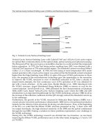
To demonstrate the proposed control method for a PM-type AGBM, an experimental setup
was constructed; it is shown schematically in Fig. 14. The rotor disc, shown in Fig. 15, has a
diameter of 50mm. Four neodymium magnets with a thickness of 1mm for each side are
mounted to the disc’s surfaces to create two pole pairs. In this paper, only rotational motion of
the rotor and translation of the stator along the z axis are considered, hence for a more simple
experiment, the rotor is supported by two radial ball bearings that restrict the radial motion.
The stator, shown in Fig. 16, has a core diameter 50 mm and six concentrated wound poles,
each with 200 coil turns. The stators can slide on the linear guide to ensure a desired air gap
between the rotor and the two stators. A DC generator (Sanyo T402) is installed to give the
load torque. A rotary encoder (Copal RE30D) measures the rotor angle and an eddy-current-
type displacement sensor (Shinkawa VC-202N) measures the axial position.
Magnetic Bearings, Theory and Applications78

The control hardware of the AGBM drive is based on a dSPACE DS1104 board dedicated to
the control of electrical drives. It includes PWM units, general purpose input/output units

(8 ADC and 8 DAC), and an encoder interface. The DS1104 reads the displacement signal
from the displacement sensor via an A/D converter, and the rotor angle position and speed
from the encoder via an encoder interface. Two motor phase currents are sensed, rescaled,
and converted to digital values via the A/D converters. The DS1104 then calculates
reference currents using the rotation control and axial position control algorithms and sends
its commands to the three-phase inverter boards. The AGBM is supplied by two three-phase
PWM inverters with a switching frequency of 20 kHz.

Stator phase resistance R
s

2.6 
Effective inductance per unit gap in d axis
0
s
d
L


8.2e-6 Hm
Effective inductance per unit gap in q axis
0sq
L


9.6e-6 Hm
Leakage inductance L
sl
6e-3 H
Inertial moment of rotor J 0.00086 kgm

2
Number of pole pairs P 1
Permanent magnet flux
m
λ

0.0126 Wb
Table 1. Parameters of salient pole AGBM


Fig. 14. Picture of the experimental setup


Fig. 15. Picture of the rotor of the AGBM Fig. 16. Picture of the stator of the AGBM

4.2 Response of Speed and Axial Displacement
Fig. 17 shows the axial displacement at 0 rpm. The original displacement is set to 0.32 mm,
and at the time of 0.45 s, the axial position controller starts to work. In transient state, the
maximum error is 0.05 mm, much smaller than the air gap at the equilibrium point (g
0
=
1.7mm) and the settling time is about 0.05 s. After that, the displacement is almost zero in a
steady state, i.e. the air gaps between stators and rotor are equal (
1 2 0
g
g g

 ). The rotor
now stands in the middle of two stators.

Fig. 17. Response of axial displacement at zero speed

Fig. 18 describes the change in the speed from zero to 6000 rpm and vice versa when the
displacement is zero and the limited current is ±5A. The AGBM does not bear any load.
With small starting time (about 0.7s) and stopping time (about 0.4s) the AGBM drive shows
its good dynamic response.


Fig. 18. Response of speed at zero displacement
Salient pole permanent magnet axial-gap self-bearing motor 79

The control hardware of the AGBM drive is based on a dSPACE DS1104 board dedicated to
the control of electrical drives. It includes PWM units, general purpose input/output units
(8 ADC and 8 DAC), and an encoder interface. The DS1104 reads the displacement signal
from the displacement sensor via an A/D converter, and the rotor angle position and speed
from the encoder via an encoder interface. Two motor phase currents are sensed, rescaled,
and converted to digital values via the A/D converters. The DS1104 then calculates
reference currents using the rotation control and axial position control algorithms and sends
its commands to the three-phase inverter boards. The AGBM is supplied by two three-phase
PWM inverters with a switching frequency of 20 kHz.

Stator phase resistance R
s

2.6


Effective inductance per unit gap in d axis
0

s
d
L


8.2e-6 Hm
Effective inductance per unit gap in q axis
0
s
q
L


9.6e-6 Hm
Leakage inductance L
sl
6e-3 H
Inertial moment of rotor J 0.00086 kgm
2
Number of pole pairs P 1
Permanent magnet flux
m
λ

0.0126 Wb
Table 1. Parameters of salient pole AGBM


Fig. 14. Picture of the experimental setup

Fig. 15. Picture of the rotor of the AGBM Fig. 16. Picture of the stator of the AGBM

4.2 Response of Speed and Axial Displacement
Fig. 17 shows the axial displacement at 0 rpm. The original displacement is set to 0.32 mm,
and at the time of 0.45 s, the axial position controller starts to work. In transient state, the
maximum error is 0.05 mm, much smaller than the air gap at the equilibrium point (g
0
=
1.7mm) and the settling time is about 0.05 s. After that, the displacement is almost zero in a
steady state, i.e. the air gaps between stators and rotor are equal (
1 2 0
g
g g  ). The rotor
now stands in the middle of two stators.


Fig. 17. Response of axial displacement at zero speed

Fig. 18 describes the change in the speed from zero to 6000 rpm and vice versa when the
displacement is zero and the limited current is ±5A. The AGBM does not bear any load.
With small starting time (about 0.7s) and stopping time (about 0.4s) the AGBM drive shows
its good dynamic response.


Fig. 18. Response of speed at zero displacement
Magnetic Bearings, Theory and Applications80

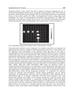
Figs. 19 and 20 show response of the axial displacement and the speed when the AGBM starts
to work. Initial displacement error is adjusted to 0.32mm, and the reference speed is 1500 rpm.

When the AGBM operates, the displacement jumps immediately to zero. At the same time, the
rotor speed increases and reaches 1500 rpm after 0.5s without influence of each other.
From above experimental results, it is obvious that the axial displacement and the speed are
controlled independently with each other.
Fig. 21 illustrates the change of the direct axis current i
d
, the quadrate axis current i
q
, and the
displacement when the motor speed changes from 1000 rpm to 1500 rpm and vice versa. The
limited currents are set to ±3A. The AGBM drive works with rotational load. The rotational
load is created by closing the terminals of a DC generator using a 1 Ω resistor. When the
reference speed is changed from 1000 rpm to 1500 rpm, the q-axis current increases to the
limited current. At the speed of 1500 rpm, the q-axis current is about 2.5A. Due to the
influence of the q-axis current as shown in equation (18), there is little higher vibration in the
displacement and the d-axis current at 1500 rpm. However, the displacement error is far
smaller than the equilibrium air gap g
0
, therefore the influence can be neglected.


Fig. 19. Response of speed at start


Fig. 20. Response of axial displacement at start




Fig. 21. Currents and displacement when rotor speed was changed

Salient pole permanent magnet axial-gap self-bearing motor 81

Figs. 19 and 20 show response of the axial displacement and the speed when the AGBM starts
to work. Initial displacement error is adjusted to 0.32mm, and the reference speed is 1500 rpm.
When the AGBM operates, the displacement jumps immediately to zero. At the same time, the
rotor speed increases and reaches 1500 rpm after 0.5s without influence of each other.
From above experimental results, it is obvious that the axial displacement and the speed are
controlled independently with each other.
Fig. 21 illustrates the change of the direct axis current i
d
, the quadrate axis current i
q
, and the
displacement when the motor speed changes from 1000 rpm to 1500 rpm and vice versa. The
limited currents are set to ±3A. The AGBM drive works with rotational load. The rotational
load is created by closing the terminals of a DC generator using a 1 Ω resistor. When the
reference speed is changed from 1000 rpm to 1500 rpm, the q-axis current increases to the
limited current. At the speed of 1500 rpm, the q-axis current is about 2.5A. Due to the
influence of the q-axis current as shown in equation (18), there is little higher vibration in the
displacement and the d-axis current at 1500 rpm. However, the displacement error is far
smaller than the equilibrium air gap g
0
, therefore the influence can be neglected.


Fig. 19. Response of speed at start


Fig. 20. Response of axial displacement at start

Fig. 21. Currents and displacement when rotor speed was changed
Magnetic Bearings, Theory and Applications82

5. Conclusion
This chapter introduces and explains a vector control of the salient two-pole AGBM drives
as required for high-performance motion control in many industrial applications.
Firstly, a general dynamic model of the AGBM used for vector control is developed, in
which the saliency of the rotor is considered. The model development is based on the
reference frame theory, in which all the motor electrical variables is transformed to a rotor
field-oriented reference frame (d,q reference frame). As seen from the d,q reference frame
rotating with synchronous speed, all stator and rotor variables become constant in steady
state. Thus, dc values, very practical regarding DC motor control strategies, are obtained.
Furthermore, by using this transformation, the mutual magnetic coupling between d- and q-
axes is eliminated. The stator current in d-axis is only active in the affiliated windings of the
d-axis, and the same applies for the q-axis.
Secondly, the vector control technique for the AGBM drives is presented in detail. In spite of
many different control structures available, the cascaded structure, inner closed-loop current
control and overlaid closed-loop speed and axial position control, is chosen. This choice
guarantees that the AGBM drive is closed to the modern drives, which were developed for
the conventional motors. Furthermore, the closed-loop vector control method for the axial
position and the speed is developed in the way of eliminating the influence of the reluctance
torque. The selection of suitable controller types and the calculation of the controller
parameters, both depending on the electrical and mechanical behavior of the controlled
objects, are explicitly evaluated.
Finally, the AGBM was fabricated with an inset PM type rotor, and the vector control with
decoupled d- and q-axis current controllers was implemented based on dSpace DS1104 and
Simukink/Matlab. The results confirm that the motor can perform both functions of motor

and axial bearing without any additional windings. The reluctance torque and its influence
are rejected entirely. Although, there is very little interference between the axial position
control and speed control in high speed range and high rotational load, the proposed AGBM
drive can be used for many kind of applications, which require small air gap, high speed
and levitation force.

6. References

Aydin M.; Huang S. and Lipo T. A. (2006). Torque quality and comparison of internal and
external rotor axial flux surface-magnet disc machines. IEEE Transactions on
Industrial Electronics, Vol. 53, No. 3, June 2006, pp. 822-830.
Chiba A.; Fukao T.; Ichikawa O.; Oshima M., Takemoto M. and Dorrell D.G. (2005). Magnetic
Bearings and Bearingless Drives, 1
st
edition, Elsevier, Burlington, 2005.
Dussaux M. (1990). The industrial application of the active magnetic bearing technology,
Proceedings of the 2nd International Symposium on Magnetic Bearings, pp. 33-38, Tokyo,
Japan, July 12–14, 1990.
Fitzgerald A. E.; C. Kingsley Jr. and S. D. Uman (1992). Electric Machinery, 5
th
edition,
McGraw-Hill, New York,1992.
Gerd Terörde (2004). Electrical Drives and Control Techniques, first edition, ACCO, Leuven,
2004.

Grabner, H.; Amrhein, W.; Silber, S. and Gruber, W. (2010). Nonlinear Feedback Control of a
Bearingless Brushless DC Motor. IEEE/ASME Transactions on Mechatronics, Vol. 15,
No. 1, Feb. 2010, pp. 40 – 47.
Horz, M.; Herzog, H G. and Medler, N., (2006). System design and comparison of
calculated and measured performance of a bearingless BLDC-drive with axial flux

path for an implantable blood pump. Proceedings of International Symposium on
Power Electronics, Electrical Drives, Automation and Motion, (SPEEDAM), pp.1024 –
1027, May 2006.
Kazmierkowski M. P. and Malesani L. (1998). Current control techniques for three-phase
voltage-source PWM converters: a survey. IEEE Transactions on Industrial
Electronics, Vol. 45, No. 5, Oct. 1998, pp. 691-703.
Marignetti F.; Delli Colli V. and Coia Y. (2008). Design of Axial Flux PM Synchronous
Machines Through 3-D Coupled Electromagnetic Thermal and Fluid-Dynamical
Finite-Element Analysis," IEEE Transactions on Industrial Electronics, Vol. 55, No. 10,
pp. 3591-3601, Oct 2008.
Nguyen D. Q. and Ueno S. (2009). Axial position and speed vector control of the inset
permanent magnet axial gap type self bearing motor. Proceedings. of the
International Conference on Advanced Intelligent Mechatronics (AIM2009), pp. 130-135,
Singapore, July 2009. (b)
Nguyen D. Q. and Ueno S. (2009). Sensorless speed control of a permanent magnet type
axial gap self bearing motor. Journal of System Design and Dynamics, Vol. 3, No. 4,
July 2009, pp. 494-505. (a)
Okada Y.; Dejima K. and Ohishi T. (1995). Analysis and comparison of PM synchronous
motor and induction motor type magnetic bearing, IEEE Transactions on Industry
Applications, vol. 32, Sept./Oct. 1995, pp. 1047-1053.
Okada, Y.; Yamashiro N.; Ohmori K.; Masuzawa T.; Yamane T.; Konishi Y. and Ueno S.
(2005). Mixed flow artificial heart pump with axial self-bearing motor. IEEE/ASME
Transactions on Mechatronics, Vol. 10, No. 6, Dec. 2005, pp. 658 – 665.
Oshima M.; Chiba A.; Fukao T. and Rahman M. A. (1996). Design and Analysis of
Permanent Magnet-Type Bearingless Motors. IEEE Transaction on Industrial
Electronics, Vol. 43, No. 2, pp. 292-299, Apr. 1996. (b)
Oshima M.; Miyazawa S.; Deido T.; Chiba A.; Nakamura F.; and Fukao T. (1996).
Characteristics of a Permanent Magnet Type Bearingless Motor. IEEE Transactions
on Industry Applications, Vol. 32, No. 2, pp. 363-370, Mar./Apr. 1996. (a)
Schneider, T. and Binder, A. (2007). Design and Evaluation of a 60000 rpm Permanent

Magnet Bearingless High Speed Motor. Proceedings on International Conference on
Power Electronics and Drive Systems, pp. 1 – 8, Bangkok, Thailand, Nov. 2007.
Ueno S. and Okada Y. (1999). Vector control of an induction type axial gap combined motor-
bearing. Proceedings of the IEEE International Conference on Advanced Intelligent
Mechatronics, Sept. 19-23, 1999, Atlanta, USA, pp. 794-799.
Ueno S. and Okada Y. (2000). Characteristics and control of a bidirectional axial gap
combined motor-bearing. IEEE Transactions on Mechatronics, Vol. 5, No. 3, Sept.
2000, pp. 310-318.
Zhaohui Ren and Stephens L.S. (2005). Closed-loop performance of a six degree-of-freedom
precision magnetic actuator, IEEE/ASME Transactions on Mechatronics, Vol. 10, No.
6, Dec. 2005 pp. 666 – 674.
Salient pole permanent magnet axial-gap self-bearing motor 83

5. Conclusion
This chapter introduces and explains a vector control of the salient two-pole AGBM drives
as required for high-performance motion control in many industrial applications.
Firstly, a general dynamic model of the AGBM used for vector control is developed, in
which the saliency of the rotor is considered. The model development is based on the
reference frame theory, in which all the motor electrical variables is transformed to a rotor
field-oriented reference frame (d,q reference frame). As seen from the d,q reference frame
rotating with synchronous speed, all stator and rotor variables become constant in steady
state. Thus, dc values, very practical regarding DC motor control strategies, are obtained.
Furthermore, by using this transformation, the mutual magnetic coupling between d- and q-
axes is eliminated. The stator current in d-axis is only active in the affiliated windings of the
d-axis, and the same applies for the q-axis.
Secondly, the vector control technique for the AGBM drives is presented in detail. In spite of
many different control structures available, the cascaded structure, inner closed-loop current
control and overlaid closed-loop speed and axial position control, is chosen. This choice
guarantees that the AGBM drive is closed to the modern drives, which were developed for
the conventional motors. Furthermore, the closed-loop vector control method for the axial

position and the speed is developed in the way of eliminating the influence of the reluctance
torque. The selection of suitable controller types and the calculation of the controller
parameters, both depending on the electrical and mechanical behavior of the controlled
objects, are explicitly evaluated.
Finally, the AGBM was fabricated with an inset PM type rotor, and the vector control with
decoupled d- and q-axis current controllers was implemented based on dSpace DS1104 and
Simukink/Matlab. The results confirm that the motor can perform both functions of motor
and axial bearing without any additional windings. The reluctance torque and its influence
are rejected entirely. Although, there is very little interference between the axial position
control and speed control in high speed range and high rotational load, the proposed AGBM
drive can be used for many kind of applications, which require small air gap, high speed
and levitation force.

6. References

Aydin M.; Huang S. and Lipo T. A. (2006). Torque quality and comparison of internal and
external rotor axial flux surface-magnet disc machines. IEEE Transactions on
Industrial Electronics, Vol. 53, No. 3, June 2006, pp. 822-830.
Chiba A.; Fukao T.; Ichikawa O.; Oshima M., Takemoto M. and Dorrell D.G. (2005). Magnetic
Bearings and Bearingless Drives, 1
st
edition, Elsevier, Burlington, 2005.
Dussaux M. (1990). The industrial application of the active magnetic bearing technology,
Proceedings of the 2nd International Symposium on Magnetic Bearings, pp. 33-38, Tokyo,
Japan, July 12–14, 1990.
Fitzgerald A. E.; C. Kingsley Jr. and S. D. Uman (1992). Electric Machinery, 5
th
edition,
McGraw-Hill, New York,1992.
Gerd Terörde (2004). Electrical Drives and Control Techniques, first edition, ACCO, Leuven,

2004.

Grabner, H.; Amrhein, W.; Silber, S. and Gruber, W. (2010). Nonlinear Feedback Control of a
Bearingless Brushless DC Motor. IEEE/ASME Transactions on Mechatronics, Vol. 15,
No. 1, Feb. 2010, pp. 40 – 47.
Horz, M.; Herzog, H G. and Medler, N., (2006). System design and comparison of
calculated and measured performance of a bearingless BLDC-drive with axial flux
path for an implantable blood pump. Proceedings of International Symposium on
Power Electronics, Electrical Drives, Automation and Motion, (SPEEDAM), pp.1024 –
1027, May 2006.
Kazmierkowski M. P. and Malesani L. (1998). Current control techniques for three-phase
voltage-source PWM converters: a survey. IEEE Transactions on Industrial
Electronics, Vol. 45, No. 5, Oct. 1998, pp. 691-703.
Marignetti F.; Delli Colli V. and Coia Y. (2008). Design of Axial Flux PM Synchronous
Machines Through 3-D Coupled Electromagnetic Thermal and Fluid-Dynamical
Finite-Element Analysis," IEEE Transactions on Industrial Electronics, Vol. 55, No. 10,
pp. 3591-3601, Oct 2008.
Nguyen D. Q. and Ueno S. (2009). Axial position and speed vector control of the inset
permanent magnet axial gap type self bearing motor. Proceedings. of the
International Conference on Advanced Intelligent Mechatronics (AIM2009), pp. 130-135,
Singapore, July 2009. (b)
Nguyen D. Q. and Ueno S. (2009). Sensorless speed control of a permanent magnet type
axial gap self bearing motor. Journal of System Design and Dynamics, Vol. 3, No. 4,
July 2009, pp. 494-505. (a)
Okada Y.; Dejima K. and Ohishi T. (1995). Analysis and comparison of PM synchronous
motor and induction motor type magnetic bearing, IEEE Transactions on Industry
Applications, vol. 32, Sept./Oct. 1995, pp. 1047-1053.
Okada, Y.; Yamashiro N.; Ohmori K.; Masuzawa T.; Yamane T.; Konishi Y. and Ueno S.
(2005). Mixed flow artificial heart pump with axial self-bearing motor. IEEE/ASME
Transactions on Mechatronics, Vol. 10, No. 6, Dec. 2005, pp. 658 – 665.

Oshima M.; Chiba A.; Fukao T. and Rahman M. A. (1996). Design and Analysis of
Permanent Magnet-Type Bearingless Motors. IEEE Transaction on Industrial
Electronics, Vol. 43, No. 2, pp. 292-299, Apr. 1996. (b)
Oshima M.; Miyazawa S.; Deido T.; Chiba A.; Nakamura F.; and Fukao T. (1996).
Characteristics of a Permanent Magnet Type Bearingless Motor. IEEE Transactions
on Industry Applications, Vol. 32, No. 2, pp. 363-370, Mar./Apr. 1996. (a)
Schneider, T. and Binder, A. (2007). Design and Evaluation of a 60000 rpm Permanent
Magnet Bearingless High Speed Motor. Proceedings on International Conference on
Power Electronics and Drive Systems, pp. 1 – 8, Bangkok, Thailand, Nov. 2007.
Ueno S. and Okada Y. (1999). Vector control of an induction type axial gap combined motor-
bearing. Proceedings of the IEEE International Conference on Advanced Intelligent
Mechatronics, Sept. 19-23, 1999, Atlanta, USA, pp. 794-799.
Ueno S. and Okada Y. (2000). Characteristics and control of a bidirectional axial gap
combined motor-bearing. IEEE Transactions on Mechatronics, Vol. 5, No. 3, Sept.
2000, pp. 310-318.
Zhaohui Ren and Stephens L.S. (2005). Closed-loop performance of a six degree-of-freedom
precision magnetic actuator, IEEE/ASME Transactions on Mechatronics, Vol. 10, No.
6, Dec. 2005 pp. 666 – 674.
Magnetic Bearings, Theory and Applications84
Passive permanent magnet bearings for rotating shaft : Analytical calculation 85
Passive permanent magnet bearings for rotating shaft : Analytical
calculation
Valerie Lemarquand and Guy Lemarquand
0
Passive permanent magnet bearings for
rotating shaft : Analytical calculation
Valerie Lemarquand
*
LAPLACE. UMR5213. Universite de Toulouse
France

Guy Lemarquand
†
LAUM. UMR6613. Universite du Maine
France
1. Introduction
Magnetic bearings are contactless suspension devices, which are mainly used for rotating ap-
plications but also exist for translational ones. Their major interest lies of course in the fact that
there is no contact and therefore no friction at all between the rotating part and its support.
As a consequence, these bearings allow very high rotational speeds. Such devices have been
investigated for eighty years. Let’s remind the works of F. Holmes and J. Beams (Holmes &
Beams, 1937) for centrifuges.
The appearing of modern rare earth permanent magnets allowed the developments of passive
devices, in which magnets work in repulsion (Meeks, 1974)(Yonnet, 1978).
Furthermore, as passive magnetic bearings don’t require any lubricant they can be used in
vacuum and in very clean environments.
Their main applications are high speed systems such as turbo-molecular pumps, turbo-
compressors, energy storage flywheels, high-speed machine tool spindles, ultra-centrifuges
and they are used in watt-hour meters and other systems in which a very low friction is
required too (Hussien et al., 2005)(Filatov & Maslen, 2001).
The magnetic levitation of a rotor requires the control of five degrees of freedom. The
sixth degree of freedom corresponds to the principal rotation about the motor axis. As a
consequence of the Earnshaw’s theorem, at least one of the axes has to be controlled actively.
For example, in the case of a discoidal wheel, three axes can be controlled by passive bearings
and two axes have to be controlled actively (Lemarquand & Yonnet, 1998). Moreover, in some
cases the motor itself can be designed to fulfil the function of an active bearing (Barthod &
Lemarquand, 1995). Passive magnetic bearings are simple contactless suspension devices but
it must be emphazised that one bearing controls a single degree of freedom. Moreover, it
exerts only a stiffness on this degree of freedom and no damping.
*

†

5
Magnetic Bearings, Theory and Applications86
Permanent magnet bearings for rotating shafts are constituted of ring permanent magnets.
The simplest structure consists either of two concentric rings separated by a cylindrical air
gap or of two rings of same dimensions separated by a plane air gap. Depending on the
magnet magnetization directions, the devices work as axial or radial bearings and thus control
the position along an axis or the centering of an axis. The several possible configurations
are discussed throughout this chapter. The point is that in each case the basic part is a ring
magnet. Therefore, the values of importance are the magnetic field created by such a ring
magnet, the force exerted between two ring magnets and the stiffness associated.
The first author who carried out analytical calculations of the magnetic field created by ring
permanent magnets is Durand (Durand, 1968). More recently, many authors proposed sim-
plified and robust formulations of the three components of the magnetic field created by ring
permanent magnets (Ravaud et al., 2008)(Ravaud, Lemarquand, Lemarquand & Depollier,
2009)(Babic & Akyel, 2008a)(Babic & Akyel, 2008b)(Azzerboni & Cardelli, 1993).
Moreover, the evaluation of the magnetic field created by ring magnets is only a helpful step
in the process of the force calculation. Indeed, the force and the stiffness are the values of
importance for the design and optimization of a bearing. So, authors have tried to work out
analytical expressions of the force exerted between two ring permanent magnets (Kim et al.,
1997)(Lang, 2002)(Samanta & Hirani, 2008)(Janssen et al., 2010)(Azukizawa et al., 2008).
This chapter intends to give a detailed description of the modelling and approach used to cal-
culate analytically the force and the stiffness between two ring permanent magnets with axial
or radial polarizations (Ravaud, Lemarquand & Lemarquand, 2009a)(Ravaud, Lemarquand
& Lemarquand, 2009b). Then, these formulations will be used to study magnetic bearings
structures and their properties.
2. Analytical determination of the force transmitted between two axially polarized
ring permanent magnets.
2.1 Preliminary remark

The first structure considered is shown on Fig.1. It is constituted of two concentric axially
magnetized ring permanent magnets. When the polarization directions of the rings are an-
tiparallel, as on the figure, the bearing controls the axial position of the rotor and works as a
so called axial bearing. When the polarization directions are the same, then the device con-
trols the centering around the axis and works as a so called radial bearing. Only one of the
two configurations will be studied thoroughly in this chapter because the results of the second
one are easily deducted from the first one. Indeed, the difference between the configurations
consists in the change of one of the polarization direction into its opposite. The consequence
is a simple change of sign in all the results for the axial force and for the axial stiffness which
are the values that will be calculated.
Furthermore, the stiffness in the controlled direction is often considered to be the most inter-
esting value in a bearing. So, for an axial bearing, the axial stiffness is the point. Nevertheless,
both stiffnesses are linked. Indeed, when the rings are in their centered position, for symmetry
reasons, the axial stiffeness, K
z
, and the radial one, K
r
, verify:
2K
r
+ K
z
= 0 (1)
So, either the axial or the radial force may be calculated and is sufficient to deduct both stiff-
nesses. Thus, the choice was made for this chapter to present only the axial force and stiffness
in the sections dealing with axially polarized magnets.
J
0
r
r

r
r
u
r
u
u
z
z
z
z
z
1
2
3
4
3
1
4 2
J
Fig. 1. Axial bearing constituted of two axially magnetized ring permanent magnets. J
1
and
J
2
are the magnet polarizations
2.2 Notations
The parameters which describe the geometry of Fig.1 and its properties are listed below:
J
1
: outer ring polarization [T].

J
2
: inner ring polarization [T].
r
1
, r
2
: radial coordinates of the outer ring [m].
r
3
, r
4
: radial coordinates of the inner ring [m].
z
1
, z
2
: axial coordinates of the outer ring [m].
z
3
, z
4
: axial coordinates of the inner ring [m].
h
1
= z
2
−z
1
: outer ring height [m].

h
2
= z
4
−z
3
: inner ring height [m].
The rings are radially centered and their polarizations are supposed to be uniform.
2.3 Magnet modelling
The axially polarized ring magnet has to be modelled and two approaches are available to
do so. Indeed, the magnet can have a coulombian representation, with fictitious magnetic
charges or an amperian one, with current densities. In the latter, the magnet is modelled
by two cylindrical surface current densities k
1
and k
2
located on the inner and outer lateral
surfaces of the ring whereas in the former the magnet is modelled by two surface charge
densities located on the plane top and bottom faces of the ring.
As a remark, the choice of the model doesn’t depend on the nature of the real magnetic
source, but is done to obtain an analytical formulation. Indeed, the authors have demontrated
Passive permanent magnet bearings for rotating shaft : Analytical calculation 87
Permanent magnet bearings for rotating shafts are constituted of ring permanent magnets.
The simplest structure consists either of two concentric rings separated by a cylindrical air
gap or of two rings of same dimensions separated by a plane air gap. Depending on the
magnet magnetization directions, the devices work as axial or radial bearings and thus control
the position along an axis or the centering of an axis. The several possible configurations
are discussed throughout this chapter. The point is that in each case the basic part is a ring
magnet. Therefore, the values of importance are the magnetic field created by such a ring
magnet, the force exerted between two ring magnets and the stiffness associated.

The first author who carried out analytical calculations of the magnetic field created by ring
permanent magnets is Durand (Durand, 1968). More recently, many authors proposed sim-
plified and robust formulations of the three components of the magnetic field created by ring
permanent magnets (Ravaud et al., 2008)(Ravaud, Lemarquand, Lemarquand & Depollier,
2009)(Babic & Akyel, 2008a)(Babic & Akyel, 2008b)(Azzerboni & Cardelli, 1993).
Moreover, the evaluation of the magnetic field created by ring magnets is only a helpful step
in the process of the force calculation. Indeed, the force and the stiffness are the values of
importance for the design and optimization of a bearing. So, authors have tried to work out
analytical expressions of the force exerted between two ring permanent magnets (Kim et al.,
1997)(Lang, 2002)(Samanta & Hirani, 2008)(Janssen et al., 2010)(Azukizawa et al., 2008).
This chapter intends to give a detailed description of the modelling and approach used to cal-
culate analytically the force and the stiffness between two ring permanent magnets with axial
or radial polarizations (Ravaud, Lemarquand & Lemarquand, 2009a)(Ravaud, Lemarquand
& Lemarquand, 2009b). Then, these formulations will be used to study magnetic bearings
structures and their properties.
2. Analytical determination of the force transmitted between two axially polarized
ring permanent magnets.
2.1 Preliminary remark
The first structure considered is shown on Fig.1. It is constituted of two concentric axially
magnetized ring permanent magnets. When the polarization directions of the rings are an-
tiparallel, as on the figure, the bearing controls the axial position of the rotor and works as a
so called axial bearing. When the polarization directions are the same, then the device con-
trols the centering around the axis and works as a so called radial bearing. Only one of the
two configurations will be studied thoroughly in this chapter because the results of the second
one are easily deducted from the first one. Indeed, the difference between the configurations
consists in the change of one of the polarization direction into its opposite. The consequence
is a simple change of sign in all the results for the axial force and for the axial stiffness which
are the values that will be calculated.
Furthermore, the stiffness in the controlled direction is often considered to be the most inter-
esting value in a bearing. So, for an axial bearing, the axial stiffness is the point. Nevertheless,

both stiffnesses are linked. Indeed, when the rings are in their centered position, for symmetry
reasons, the axial stiffeness, K
z
, and the radial one, K
r
, verify:
2K
r
+ K
z
= 0 (1)
So, either the axial or the radial force may be calculated and is sufficient to deduct both stiff-
nesses. Thus, the choice was made for this chapter to present only the axial force and stiffness
in the sections dealing with axially polarized magnets.
J
0
r
r
r
r
u
r
u
u
z
z
z
z
z
1

2
3
4
3
1
4 2
J
Fig. 1. Axial bearing constituted of two axially magnetized ring permanent magnets. J
1
and
J
2
are the magnet polarizations
2.2 Notations
The parameters which describe the geometry of Fig.1 and its properties are listed below:
J
1
: outer ring polarization [T].
J
2
: inner ring polarization [T].
r
1
, r
2
: radial coordinates of the outer ring [m].
r
3
, r
4

: radial coordinates of the inner ring [m].
z
1
, z
2
: axial coordinates of the outer ring [m].
z
3
, z
4
: axial coordinates of the inner ring [m].
h
1
= z
2
−z
1
: outer ring height [m].
h
2
= z
4
−z
3
: inner ring height [m].
The rings are radially centered and their polarizations are supposed to be uniform.
2.3 Magnet modelling
The axially polarized ring magnet has to be modelled and two approaches are available to
do so. Indeed, the magnet can have a coulombian representation, with fictitious magnetic
charges or an amperian one, with current densities. In the latter, the magnet is modelled

by two cylindrical surface current densities k
1
and k
2
located on the inner and outer lateral
surfaces of the ring whereas in the former the magnet is modelled by two surface charge
densities located on the plane top and bottom faces of the ring.
As a remark, the choice of the model doesn’t depend on the nature of the real magnetic
source, but is done to obtain an analytical formulation. Indeed, the authors have demontrated
Magnetic Bearings, Theory and Applications88
J
I
1
2
I
u
u
z
z
r
r
1
2
u
z
r
2
r
1
Fig. 2. Model of a ring magnet: amperian equivalence.

that depending on the polarization direction of the source only one of the model generally
yields an analytical formulation. So, the choice rather depends on the considered problem.
2.4 Force calculation
The force transmitted between two axially polarized ring permanent magnets is determined
by using the amperian approach. Thus, each ring is replaced by two coils of N
1
and N
2
turns
in which two currents, I
1
and I
2
, flow. Indeed, a ring magnet whose polarization is axial and
points up, with an inner radius r
1
and an outer one r
2
, can be modelled by a coil of radius
r
2
with a current I
2
flowing anticlockwise and a coil of radius r
1
with a current I
1
flowing
clockwise (Fig.2).
The equivalent surface current densities related to the coil heights h

1
and h
2
are defined as
follows for the calculations:
k
1
= N
1
I
1
/h
1
: equivalent surface current density for the coils of radii r
1
and r
2
.
k
2
= N
2
I
2
/h
2
: equivalent surface current density for the coils of radii r
3
and r
4

.
The axial force, F
z
, created between the two ring magnets is given by:
F
z
=
µ
0
k
1
k
2
2
2
∑
i=1
4
∑
j=3
(−1)
1+i+j

f
z
(r
i
, r
j
)


(2)
with
f
z
(r
i
, r
j
) = r
i
r
j

z
4
z
3

z
2
z
1

2π
0
(
˜
˜
z

−
˜
z
) cos(
˜
θ
)d
˜
zd
˜
˜
zd
˜
θ

r
2
i
+ r
2
j
−2r
i
r
j
cos(
˜
θ
) + (
˜

˜
z
−
˜
z
)
2

3
2
Parameter Definition
β
b+c
b
−c
µ
c
b
+c

c
c
−b
Table 1. Parameters in the analytical expression of the force exerted between two axially po-
larized ring magnets.
The current densities are linked to the magnet polarizations by:
k
1
=
J

1
µ
0
(3)
and
k
2
=
J
2
µ
0
(4)
Then the axial force becomes:
F
z
=
J
1
J
2
2µ
0
2
∑
i,k=1
4
∑
j,l=3
(−1)

(1+i+j+k+l)
F
i,j,k,l
(5)
with
F
i,j,k,l
= r
i
r
j
g

z
k
−z
l
, r
2
i
+ r
2
j
+ (z
k
−z
l
)
2
, −2r

i
r
j

(6)
g
(a, b, c) = A + S
A
=
a
2
−b
c
π
+

c
2
−(a
2
−b)
2
c

log

−16c
2
(c
2

−(a
2
−b)
2
)
(
3
2
)

+ log

c
2
(c
2
−(a
2
−b)
2
)
(
3
2
)

S
=
2ia
c

√
b + c

(b + c)E

arcsin


β, β
−1

−cF

arcsin


β, β
−1

+
2 a
c
√
b −c
√


c
√
µ

E

β
−1

−c
√
µK

β
−1


+

β
−1

(b − a
2
)K
[
2µ
]
+ (
a
2
−b + c)Π

2c

b
+ c − a
2
, 2µ

(7)
The special functions used are defined as follows:
K
[
m
]
is the complete elliptic integral of the first kind.
K
[
m
]
=

π
2
0
1

1
−m sin( θ)
2
dθ (8)
Passive permanent magnet bearings for rotating shaft : Analytical calculation 89
J
I

1
2
I
u
u
z
z
r
r
1
2
u
z
r
2
r
1
Fig. 2. Model of a ring magnet: amperian equivalence.
that depending on the polarization direction of the source only one of the model generally
yields an analytical formulation. So, the choice rather depends on the considered problem.
2.4 Force calculation
The force transmitted between two axially polarized ring permanent magnets is determined
by using the amperian approach. Thus, each ring is replaced by two coils of N
1
and N
2
turns
in which two currents, I
1
and I

2
, flow. Indeed, a ring magnet whose polarization is axial and
points up, with an inner radius r
1
and an outer one r
2
, can be modelled by a coil of radius
r
2
with a current I
2
flowing anticlockwise and a coil of radius r
1
with a current I
1
flowing
clockwise (Fig.2).
The equivalent surface current densities related to the coil heights h
1
and h
2
are defined as
follows for the calculations:
k
1
= N
1
I
1
/h

1
: equivalent surface current density for the coils of radii r
1
and r
2
.
k
2
= N
2
I
2
/h
2
: equivalent surface current density for the coils of radii r
3
and r
4
.
The axial force, F
z
, created between the two ring magnets is given by:
F
z
=
µ
0
k
1
k

2
2
2
∑
i=1
4
∑
j=3
(−1)
1+i+j

f
z
(r
i
, r
j
)

(2)
with
f
z
(r
i
, r
j
) = r
i
r

j

z
4
z
3

z
2
z
1

2π
0
(
˜
˜
z
−
˜
z
) cos(
˜
θ
)d
˜
zd
˜
˜
zd

˜
θ

r
2
i
+ r
2
j
−2r
i
r
j
cos(
˜
θ
) + (
˜
˜
z
−
˜
z
)
2

3
2
Parameter Definition
β

b+c
b−c
µ
c
b+c

c
c−b
Table 1. Parameters in the analytical expression of the force exerted between two axially po-
larized ring magnets.
The current densities are linked to the magnet polarizations by:
k
1
=
J
1
µ
0
(3)
and
k
2
=
J
2
µ
0
(4)
Then the axial force becomes:
F

z
=
J
1
J
2
2µ
0
2
∑
i,k=1
4
∑
j,l=3
(−1)
(1+i+j+k+l)
F
i,j,k,l
(5)
with
F
i,j,k,l
= r
i
r
j
g

z
k

−z
l
, r
2
i
+ r
2
j
+ (z
k
−z
l
)
2
, −2r
i
r
j

(6)
g
(a, b, c) = A + S
A
=
a
2
−b
c
π
+


c
2
−(a
2
−b)
2
c

log

−16c
2
(c
2
−(a
2
−b)
2
)
(
3
2
)

+ log

c
2
(c

2
−(a
2
−b)
2
)
(
3
2
)

S
=
2ia
c
√
b + c

(b + c)E

arcsin


β, β
−1

−cF

arcsin



β, β
−1

+
2 a
c
√
b −c
√


c
√
µ
E

β
−1

−c
√
µK

β
−1


+


β
−1

(b − a
2
)K
[
2µ
]
+ (
a
2
−b + c)Π

2c
b + c − a
2
, 2µ

(7)
The special functions used are defined as follows:
K
[
m
]
is the complete elliptic integral of the first kind.
K
[
m
]

=

π
2
0
1

1 − m sin(θ)
2
dθ (8)
Magnetic Bearings, Theory and Applications90
F
[
φ, m
]
is the incomplete elliptic integral of the first kind.
F
[
φ, m
]
=

φ
0
1

1 − m sin(θ)
2
dθ (9)
E

[
φ, m
]
is the incomplete elliptic integral of the second kind.
E
[
φ, m
]
=

φ
0

1 − m sin(θ)
2
dθ (10)
E
[
m
]
=

π
2
0

1 − m sin(θ)
2
dθ (11)
Π

[
n, m
]
is the incomplete elliptic integral of the third kind.
Π
[
n, m
]
=
Π

n,
π
2
, m

(12)
with
Π
[
n, φ, m
]
=

φ
0
1

1 − n sin(θ)
2

1

1 − m sin(θ)
2
dθ (13)
3. Exact analytical formulation of the axial stiffness between two axially polarized
ring magnets.
The axial stiffness, K
z
existing between two axially polarized ring magnets can be calculated
by deriving the axial force transmitted between the two rings, F
z
, with regard to the axial
displacement, z:
K
z
= −
d
dz
F
z
(14)
F
z
is replaced by the integral formulation of Eq.5 and after some mathematical manipulations
the axial stiffness can be written:
K
z
=
J

1
J
2
2µ
0
2
∑
i,k=1
4
∑
j,l=3
(−1)
(1+i+j+k+l)
C
i,j,k,l
(15)
where
C
i,j,k,l
= 2
√
αE

−4r
i
r
j
α

−2

r
2
i
+ r
2
j
+ (z
k
−z
l
)
2
√
α
K

−4r
i
r
j
α

α
= (r
i
−r
j
)
2
+ (z

k
−z
l
)
2
(16)
4. Study and characteristics of axial bearings with axially polarized ring magnets
and a cylindrical air gap.
4.1 Structures with two ring magnets
This section considers devices constituted of two ring magnets with antiparallel polarization
directions. So, the devices work as axial bearings. The influence of the different parameters
of the geometry on both the axial force and stiffness is studied.
4.1.1 Geometry
The device geometry is shown on Fig.1. The radii remain the same as previously defined. Both
ring magnets have the same axial dimension, the height h
1
= h
2
= h. The axial coordinate,
z, characterizes the axial displacement of the inner ring with regard to the outer one. The
polarization of the magnets is equal to 1T.
The initial set of dimensions for each study is the following:
r
1
= 25mm, r
2
= 28mm, r
3
= 21mm, r
4

= 24mm, h = 3mm
Thus the initial air gap is 1mm wide and the ring magnets have an initial square cross section
of 3
×3mm
2
.
4.1.2 Air gap influence
The ring cross section is kept constant and the radial dimension of the air gap, r
1
−r
3
, is varied
by modifying the radii of the inner ring. Fig.3 and 4 show how the axial force and stiffness are
modified when the axial inner ring position changes for different values of the air gap.
Naturally, when the air gap decreases, the modulus of the axial force for a given axial position
of the inner ring increases (except for large displacements) and so does the modulus of the
axial stiffness. Furthermore, it has to be noted that a positive stiffness corresponds to a stable
configuration in which the force is a pull-back one, whereas a negative stiffness corresponds
to an unstable position: the inner ring gets ejected!
 4
 2
0
2
4
 60
 40
 20
0
20
40

60
z mm
Axial Force N
Fig. 3. Axial force for several air gap radial dimensions. Blue: r
1
= 25mm, r
2
= 28mm, r
3
=
21mm, r
4
= 24mm, h = 3mm Air gap 1mm, Green: Air gap 0.5mm , Red: Air gap 0.1mm
4.1.3 Ring height influence
The air gap is kept constant as well as the ring radii and the height of the rings is varied.
Fig.5 and 6 show how the axial force and stiffness are modified. When the magnet height
decreases, the modulus of the axial force for a given axial position of the inner ring decreases.
This is normal, as the magnet volume also decreases.
The study of the stiffness is carried out for decreasing ring heights (Fig.6) but also for
increasing ones (Fig.7). As a result, the stiffness doesn’t go on increasing in a significant way
above a given ring height. This means that increasing the magnet height, and consequently