Mobile Ad Hoc Networks Applications Part 14 pdf

Mobile Ad-Hoc Networks: Applications

446



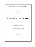
(a) DSDV (b) DSR



(c) AODV (d) AOMDV



(e) OLSR
Fig. 11. Throughput measurement in the random topology
The Effect of Packet Losses and Delay on TCP Traffic over Wireless Ad Hoc Networks

447
5.3.3 Throughput measurement
The TCP variants over DSDV achieve a higher throughput by a factor of almost 1.5 on
average compared to others as shown in Fig. 11(a). The better stability of throughput for the
TCP variants could be encountered in proactive routing protocols DSDV and OLSR (Fig.
11(e)). When the number of nodes increases, the possibility of congestion and the contention
at the MAC layer increase in the network. However, when the routing layer protocols
receive the collision reports from the link layer, they re-discover routes by sending the
broadcast messages throughout the network. Therefore, in Fig. 11(c), AODV suffers a lower
throughput if compared to others. Another thing is that DSR suffers the instability
throughput for all TCP variants because when the node density and the number of
connections increase, the stale route problem of DSR comes active and makes the
performance worse (Fig. 11(b)).

6. Conclusion
In this chapter, we analyze the performance of TCP variants across ad hoc routing protocols
in static and mobile ad hoc environments. The performance of TCP variants vary depending
on the routing protocols, their core mechanisms and background changes, such as the node
mobility, node speed, pause time and number of tcp connections and network topologies. In
the chain topology, all of the TCP variants achieve a significantly lower delay over AODV
routing protocol in both environments. Moreover, AODV provides a higher throughput for
all TCP variants, especially for Vegas in both environments. One interesting thing is that
AODV always achieves a lower delay, it suffers a higher delay than others in the grid
topology. In the grid topology, although TCP variants have the lowest delay over DSDV in
both environments, in the random topology, TCP variants incur a lower packet losses over
DSR and OLSR, and encounter a lower delay over DSDV. On the other hand, DSDV and
OLSR provide the highest data transfer rate (i.e. throughput) for all TCP variants in random
topology. Among all TCP variants, Vegas is the best transport protocol and performs better
than others in most situations.
7. Acknowledgement
This work is supported in part by University of Malaya Research Grand (UMRG) under
grant RG024/09ICT.
8. References
BonnMotion: a Mobility Scenario Generation and Analysis Tool (2009). Available from:
/>Motion_Docu.pdf.
Ahuja, A.; Agarwal, S.; Singh, J. P. & Shorey, R. (2000). Performance of TCP over Different
Routing Protocols in Mobile Ad Hoc Networks, IEEE 51
st
Vehicular Technology
Conference, pp. 2315-2319, 0-7803-5721-3, Tokyo, May 2000, Japan.
Allman, M. (1999). TCP Congestion Control, Request for comment 2581.
Mobile Ad-Hoc Networks: Applications

448

Anastasi, G.; Ancillotti, E.; Conti, M. & Passarella, A. (2007). Experimental Analysis of TCP
Performance in Static Multi-hop Ad Hoc Networks, In: Multi-hop Ad Hoc Networks
from Theory to Reality, Conti, M.; Crowcroft, J. & Passarella, A. (Ed.), page number
(97-114), Nova Science, 1-60021-605-6, New York.
Boppana, R. & Konduru, S. (2001). An Adaptive Distance Vector Routing Algorithm for
Mobile Ad Hoc Networks, IEEE Infocom, pp. 1753-1762, 0-7803-7016-3, Anchorage,
April 2001, Alaska.
Brakno, L. S.; O'Malley, S. W. & Peterson, L. L. (1994). TCP Vegas: new techniques for
congestion detection and avoidance, ACM SIGCOMM Computer Communication
Review, Vol. 24, No. 4, (October 1994) page number (24-35), 0146-4833.
Camp, T., Boleng, J. & Davies, V. (2002). A survey of mobility models for ad hoc network
research, Wireless Communications and Mobile Computing Special Issue on Mobile Ad
Hoc Networking: Research, Trends and Applications, Vol. 2, No. 5, (August 2002) page
number (483-502), 1530-8669.
Chandran, K.; Raghunathan, S.; Venkatesan, S. & Prakash, R. (2001). A Feedback Based
Scheme for Improving TCP Performance in Ad Hoc Wireless Networks, IEEE
Personal Communication Magazine, Special Issue on Ad Hoc Networks, Vol. 8, No. 6,
(August 2001) page number (34-39), 1070-9916.
Clausen, T. & Jacquet, P. (2003). Optimized Link State Routing Protocol (OLSR), Request for
Comments 3626.
Dube, R.; Rais, C. D.; Wang, K-Y. & Tripathi, S. K. (1997). Signal Stability-based Adaptive
(SSA) Routing for Ad Hoc Mobile Networks. IEEE Personal Communications
Magazine, Vol. 4, No. 1, (February 1997) page number (36-45), 1070-9916.
Dyer, T. D. & Boppana, R. V. (2001). A Comparison of TCP Performance over Three Routing
Protocols for Mobile Ad Hoc Networks, ACM Symposium on Mobile Ad Hoc
Networking & Computing, pp. 56-66, 1-58113-428-2, Long Beach, October 2001, ACM,
California.
El-Sayed, H. M. (2005). Performance evaluation of TCP in mobile ad hoc networks, The
Second International Conference on Innovations in Information Technology, September
2005.

Floyd, S. & Henderson, T. (1999). The NewReno Modification to TCP's Fast Recovery
Algorithm, Request for Comments 2582.
Gerla, M.; Sanadidi, M. Y.; Zanella, R. W.; Casetti, A. & Mascolo, S. (2002). TCP Westwood:
congestion window control using bandwidth estimation. IEEE Global
Telecommunications Conference, pp. 1698-1702, 0-7803-7206-9, San Antonio, August
2002, IEEE Computer Society,TX.
Gupta, A.; Wormsbecker, I. & Williamson, C. (2004). Experimental Evaluation of TCP
Performance in Multi-hop Wireless Ad Hoc Networks, Proceedings of IEEE Annual
Internation Symposium on Modeling, Analysis, and Simulation of Computer and
Telecommunications Systems, pp. 3-11, 0-7695-2251-3, Volendam, October 2004, IEEE
Computer Society, The Netherlands.
Holland, G. & Vaidya, N. (2002). Analysis of TCP Performance over Mobile Ad Hoc
Networks, Wireless Networks, Vol. 8, No. 2/3 (March 2002) page number (275-288),
1002-0038.
The Effect of Packet Losses and Delay on TCP Traffic over Wireless Ad Hoc Networks

449
Johnson, D.; Hu, Y. & Maltz, D. (2007). The Dynamic Source Routing Protocol (DSR) for
Mobile Ad Hoc Networks for IPv4, Request for comment 4728.
Kawadia, V. & Kumar, P. (2005). Experimental investigation into TCP Performance over
Wireless Multihop Networks, SIGCOMM Workshops, pp. 22-25, 1-59593-026-4,
Philadelphia, August 2005, ACM, USA.
Kim, D.; Bae, H. & Song, J. (2005). Analysis of the Interaction between TCP Variants and
Routing Protocols in MANETs, Proceedings of the IEEE International Conference on
Parallel Processing Workshops, pp. 380-386, 0-7695-2381-1, University of Oslo, June
2005, IEEE Computer Society, Norway.
Lim, H.; Xu, K. & Gerla, M. (2003). TCP performance over multipath routing in mobile ad
hoc networks, IEEE International Conference on Communication, pp. 1064-1068, 0-
7803-7802-4, Anchorage, May 2003, IEEE Computer Society, Alaska.
Marina, M. K. & Das, S. R. (2006). Ad hoc on-demand multipath distance vector routing,

Wireless Communications and Mobile Computing, Vol. 6, No. 7, (November 2006) page
number (969-988), 1530-8669.
Mathis, M. & Mahdavi, J. (1996). TCP Selective Acknowledgement Options, Request for
comment 2018.
McCanne, S. & Floyd, S. VINT Group, Network Simulator Ns-2. Source code:

Mondal, S. A. & Luqman, F. B. (2007). Improving TCP performance over wired-wireless
networks, Computer Networks, Vol. 51, No. 13, (September 2007), page number
(3799-3811), 1389-1286.
Oo, M. Z. & Othman, M. (2010). Performance Comparisons of AOMDV and OLSR Routing
Protocols for Mobile Ad Hoc Network, 2010 Second International Conference on
Computer Engineering and Applications, pp. 129-133, 978-0-7695-3982-9, Bali Island,
March 2010, Indonesia.
Osipov, E. & Tschudin, C. (2006). Evaluating the Effect of Ad Hoc Routing on TCP
Performance in IEEE 802.11 Based MANETs, In: Next Generation Teletraffic and
Wired/Wireless Advanced Networking, Koucheryacy, Y.; Harju, J. & Lversen,
V. B. (Ed.), page number (298-312), Springer Berlin, 978-3-540-34429-2,
Heidelberg.
Perkins, C.; Belding-Royer, E. & Das., S. (2003). Ad hoc on-demand distance vector routing
(AODV), Request for Comments 3561.
Perkins, C. E. & Watson, T. J. (1994). Highly dynamic destination sequenced distance vector
routing (DSDV) for mobile computers, ACM SIGCOMM Computer Communication
Review, Vol. 24, No. 4, (October 1994) page number (234-244), 0146-4833.
Postel, J. (1981). Transmission Control Protocol (TCP), Request for comment 793.
Rakabawy, E. S.; Lindemann, C. & Vernon, M. (2005). Improving TCP Performance for
Multihop Wireless Networks, IEEE International Conference on Dependable Systems
and Networks, pp. 684-693, 0-7695-2282-3, Yokohama, June 2005, IEEE Computer
Society, Japan.
Sakib, A. M. (2009). Improving performance of TCP over mobile wireless networks, Wireless
Networks, Vol. 15, No. 3, (April 2009) page number (331-340), 1002-0038.

Mobile Ad-Hoc Networks: Applications

450
Stevens, W. (1997). TCP Slow Start, Congestion Avoidance, Fast Retransmit, Request for
comment 2001.
Tseng, Y C.; Ni, S Y.; Chen, Y S. & Sheu, J P. (2002). The broadcast storm problem in a
mobile ad hoc network. Wireless Networks, Vol. 8, No. 2/3, (March-May 2002) page
number (153-167), 1002-0038.
Xu, S. & Saadawi, T. (2000). Performance Evaluation of TCP Algorithms in Multi-hop
Wireless Packet Networks, Wireless Communications and Mobile Computing, Vol. 2,
No. 1, (December 2001) page number (85-100), 1530-8669.
Part 5
Other Topics


1. Introduction
Even though the interest in ad hoc wireless networks has begun in the early 1970s, several
technological difficulties, particularly those related to implementation, have postponed
advances in this field until the 1990s, when important issues were investigated and solved,
including medium access control, routing, energy consumption, among others. These
advances have allowed for actual implementation and commercial deployment of wireless
communication systems based on the ad hoc concept, including wireless sensor networks,
Internet access in rural areas, etc. Despite the formidable advances in this field observed
in the last two decades, one key problem remains open and is still subject to intense research
effort: that of modeling and measuring the capacity of ad hoc networks (Andrews et al., 2008).
The intrinsic characteristics of ad hoc networks, particularly the lack of a central coordination
entity and its consequences, added to the peculiarities of the wireless communication channel,
make the estimation of capacity of ad hoc networks a challenging task. Despite the mentioned
difficulties, researchers have proposed a myriad of metrics for characterizing the capacity of
ad hoc networks under different conditions and emphasizing different aspects of the network,

as described throughout this chapter.
One of the first key results in this field was achieved by Kleinrock and Silvester (Kleinrock
& Silvester, 1978) in late 1970’s, when they investigated the relationship between capacity
and transmission radius in a network of packet radios operating under ALOHA protocol.
Takagi and Kleinrock further investigated this relationship in (Takagi & Kleinrock, 1984).
Both works were based on the metric so called expected forward progress, defined in such
way to capture the tradeoff relating the one-hop throughput and the average one-hop
length. In fact, decreasing the one-hop length has conflicting effects on throughput: it may
increase throughput due to the resulting link quality improvement, but it may also decrease
throughput, due to a larger traffic and a higher contention level caused by the consequent
larger number of hops between source and destination. Subbarao and Hughes (Subbarao
& Hughes, 2000) improved the model previously proposed, by including the effects of the
transmission system, and introduced the concept of information efficiency, defined as the
product of the expected forward progress and the spectral efficiency of the transmission
system. Nardelli and Cardieri extended the concept of information efficiency by taking into
account the effects of channel reuse and multi-hop transmissions, leading to a new metric,
named aggregate multi-hop information efficiency (Nardelli & Cardieri, 2008a; Nardelli et al.,
Paulo Cardieri
1
and Pedro Henrique Juliano Nardelli
2
1
University of Campinas
2
University of Oulu
1
Brazil
2
Finland
A Survey on the Characterization of the

Capacity of Ad Hoc Wireless Networks

20
2 Theor y and Applications of Ad Hoc Networks
2009). Based on a similar concept as that of information efficiency, Weber et al. introduced
the metric transmission capacity (Weber et al., 2005), which is related to the optimum density
of concurrent transmissions that guarantees that outage constraints are met. Simply stated,
transmission capacity is the area spectral efficiency of successful transmissions resulted
from the optimal contention density. The capacity metrics cited above, to be described in
Section 2, have in common their statistical basis, resulted from the statistical nature of several
mechanisms related to wireless communications, such as the interaction among nodes sharing
a given channel and the propagation effects.
Following a deterministic approach to characterizing capacity of ad hoc networks and
focusing on the behavior of capacity scaling laws, Gupta and Kumar introduced the
concept of transport capacity (Gupta & Kumar, 2000), which relates transmission rate and
source-destination distance. Gupta and Kumar formulated the transport capacity from the
perspective of the requirements for successful transmission, which were described according
to two interference models: the Protocol Interference Model, which is geometric-based,
and the Physical Interference Model, based on signal-to-interference ratio requirements.
Gupta and Kumar investigated the behavior of the network capacity when the number of
nodes grows (i.e., asymptotic capacity), to show that the per-node throughput decreases as
O
(1/
√
n ), where n is the number of nodes in the network. This approach was followed
by several authors to investigate the asymptotic capacity of wireless ad hoc networks in a
variety of scenarios, such as different transmission constraints (Xie & Kumar, 2004; 2006), and
with directional antennas (Sagduyu & Ephremides, 2004). Grossglauser and Tse presented an
important extension of the work of Gupta and Kumar by considering the effects of mobility
on the capacity (Grossglauser & Tse, 2002). They showed that, in a network with mobile nodes

operating under a 2-hop relaying transmission scheme, the per-node throughput capacity may
remain constant as the number of nodes in the network increases, at the cost of unbounded
packet transmission delay. This important result motivated other researchers to further
investigate the tradeoff between capacity and delay in mobile wireless networks (El Gamal
et al., 2006), (Herdtner & Chong, 2005), (Neely & Modiano, 2005). In Section 3 we will discuss
the main results on network capacity evaluation from the perspective of scaling laws.
The brief review presented above is an evidence of the complexity of the problem of
characterizing capacity of ad hoc networks, leading to a number of different metrics, with
different focuses and perspectives. While this large number of metrics is also an evidence of
the importance of this field, it may also mislead researchers looking for appropriate models
and metrics for a particular application or scenario. This chapter therefore aims at providing
readers with an overview of capacity metrics for wireless ad hoc networks, emphasizing the
rationale behind the metrics.
2. Statistical-based capacity metrics
The inherent random nature of ad hoc networks suggests a statistical approach to quantify
capacity of such networks. Specifically, a statistical approach is very useful for the
design of practical communication systems, when a set of quality requirements is imposed
by the user application in mind. In this section we will discuss some statistical-based
capacity metrics found in the literature, namely expected forward progress, information
efficiency, transmission capacity and aggregate multi-hop information efficiency metrics. The
specificities of each metric will be discussed and their application scenario will be pointed out.
454
Mobile Ad-Hoc Networks: Applications
A Survey on the Characterization of the Capacity of Ad Hoc Wireless Networks 3
2.1 Expected forward progress
As already mentioned, the work done by Kleinrock and Silvester (Kleinrock & Silvester,
1978) in the late 1970’s was one of the first attempts to model capacity of ad hoc wireless
networks (Kleinrock & Silvester, 1978). They proposed the metric expected forward progress
(EFP), measured in meters and defined as the product of the distance traveled by a packet
toward its destination and the probability that such packet is successfully received. Formally,

EFP
= d × (1 − P
out
), (1)
where d is the transmitter-receiver separation distance and P
out
is the outage probability,
i.e., the probability that the bit error rate (or other related metric) is higher than a given
threshold. In (Kleinrock & Silvester, 1978) the authors introduced the idea of modeling
network as a collection of nodes following a spatial point process, allowing for the use of tools
and properties of Stochastic Geometry (Baddeley, 2007), making possible to derive analytical
formulation relating several network parameters, such node density, propagation channel
parameters, number of hops, packet error probability, etc. In fact, a plethora of analysis was
performed based on the metric EFP (e.g. (Sousa & Silvester, 1990), (Sousa, 1990), (Zorzi &
Pupolin, 1995)).
2.2 Information efficiency
Subbarao and Hughes (Subbarao & Hughes, 2000) extended the work done by Silvester
and Kleinrock by including in the model the spectral efficiency of the transmission system,
resulting in a new metric, named information efficiency (IE), which is formally defined as the
product of EFP and the spectral efficiency η of the link connecting transmitter and receiver
nodes, or
IE
= η ×d × (1 − P
out
). (2)
Roughly speaking, IE quantifies how efficiently the information bits can travel towards its
destination.
In order to understand the tradeoff captured by the information efficiency, let us consider a
transmission system in which modulation and error-correcting coding techniques should be
selected to optimize the IE of the network. If a modulation technique with large cardinality is

used, then the spectral efficiency of the system increases, at expenses of a higher minimum
required signal-to-interference plus noise ratio (SINR) to achieve a given packet error
probability. This higher required SINR clearly increases the outage probability P
out
. Error
correcting coding also plays an important role in this tradeoff, as it can reduce the minimum
required SINR, at the expenses of a higher bandwidth, reducing therefore the spectral
efficiency of the transmissions. These tradeoffs are captured by the information efficiency
metric, allowing for a joint system design involving modulation, coding, transmission range,
among other parameters. Following this approach, the performance of different transmission
schemes was investigated, such as, discrete sequence spread spectrum (Subbarao & Hughes,
2000), frequency hopping (Liang & Stark, 2000), direct sequence mobile networks (Chandra &
Hughes, 2003), direct sequence code-division multiple access with channel-adaptive routing
(Souryal et al., 2005) and coded MIMO frequency hopping CDMA (Sui & Zeidler, 2009).
It should be noted that, from the perspective of the whole network, the information efficiency
of a link does not tell us much about how efficiently the channel is being reused throughout
the network area. We will return to this point when discussing the next two metrics.
455
A Survey on The Characterization of the Capacity of Ad Hoc Wireless Networks
4 Theor y and Applications of Ad Hoc Networks
2.3 Transmission capacity
Weber et al. proposed in (Weber et al., 2005) the transmission capacity (TmC) metric of
single-hop ad hoc networks. TmC is defined as the product of the density of successful links
and their communication rates, subject to a constraint on the outage probability. Formally,
TmC
= η ×λ × (1 − P
out
), (3)
where λ is the density of active links in the network. Therefore, TmC quantifies the spatial
spectral efficiency of the network, capturing in its formulation the effects of active links

density on the outage probability. In fact, with a high density of concurrent transmissions,
information flow in the network is also higher, which is indicated by a high TmC. However,
the downside of a high density of active links is an increase in the interference level, leading
to a higher outage probability and, consequently, a lower transmission capacity. This tradeoff,
together with the ones previously presented, are the basis of the TmC framework, which
can be used to evaluate several transmission strategies with different focuses. For instance,
TmC was used to study frequency hopping spread spectrum (Weber et al., 2005), interference
cancelation (Weber, Andrews, Yang & de Veciana, 2007), threshold transmissions and channel
inversion (Weber, Andrews & Jindal, 2007), power control (Jindal et al., 2008), among many
others. In fact, TmC is one of the most flexible metrics to study single-hop ad hoc networks.
However, in multi-hop links scenarios, TmC is not an appropriate metric, as it does not take
into account the expected forward progress of packets, making this metric unsuitable to study,
for instance, the effects of different routing strategies.
2.4 Aggregate multi-hop information efficiency
In (Mignaco & Cardieri, 2006), Mignaco and Cardieri extended the work done by Subbarao
and Hughes by including the effects of spatial reuse in the definition of the IE, leading to
a new metric named aggregate information efficiency (AIE). This new metric is defined as the
sum of the IE of active links in the network per unit area. Nardelli and Cardieri further
improved the network model used to define AIE, by including the effects of retransmissions
(Nardelli & Cardieri, 2008a) and outage constraints (Nardelli & Cardieri, 2008b). Particularly,
in (Nardelli & Cardieri, 2008b) the authors make the AIE an extension of the metric TmC,
where the distance traveled by a packet is explicitly considered.
Nonetheless, the metric AIE does not yet take into account the effects of multi-hop
communication links. In (Nardelli et al., 2009), Nardelli et al. addressed such limitation
and proposed the metric aggregate multi-hop information efficiency (AMIE). The idea behind the
evolution from AIE to AMIE is to abstract multi-hop links and evaluate the AMIE based on the
end-to-end performance of multi-hop links. Formally, the aggregate multi-hop information
efficiency is defined as
AMIE
= d × η ×λ × (1 − P

out
)
h
, (4)
where h is the average number of hops between source and destination, and d, η, λ and
P
out
were already defined. The main advantage of the AMIE is to be more flexible and
general than other similar metrics. Based on this metric, several transmission schemes and
network scenarios have been investigated, such as M-QAM modulation with Reed-Solomon
coding scheme and ARQ retransmissions (Nardelli et al., 2009), different access protocols with
limited number of retransmissions and back-offs (Nardelli et al., 2010; Kaynia et al., 2010) and
different hopping strategies (Nardelli & Cardieri, 2010).
456
Mobile Ad-Hoc Networks: Applications
A Survey on the Characterization of the Capacity of Ad Hoc Wireless Networks 5
3. Capacity scaling laws
In this section, we study the capacity of wireless networks from the perspective of scaling
laws, that is, we are now interested in understanding how capacity scales as the number of
nodes in the network grows. This is an important subject to be investigated, as it exposes
how several intrinsic aspects of wireless communication, such as interference, channel reuse
and resource limitation, affect the performance of a network. Throughput, measured in
bit per second, is a typical metric of capacity of communication networks and, as such, is
one of the quantities considered in this section. However, in ad hoc wireless networks, in
their most general configuration, source and destination nodes may be far apart, such that
direct communication (single hop) is not possible, requiring a multi hop connection, with
neighboring nodes acting as relays. Clearly, multi hop connections leads to a traffic increase,
as a given packet is transmitted several times before reaching its final destination. Therefore,
source-destination separation distance must be taken into account when characterizing
capacity in wireless ad hoc networks. In this sense, a very popular capacity metric for ad

hoc networks is the transport capacity, measured in bit
·meter per second. Consider a network
with transport capacity of T bit
·meter per second. This means that the rate between two nodes
spaced one meter away from each other is T b/s. If the distance between the nodes is doubled,
then the rate decreases to T/2 b/s.
Gupta and Kumar (Gupta & Kumar, 2000) investigated the transport capacity and the
throughput capacity of wireless networks, and derived bounds that describe the behavior
of the network capacity when the number of the nodes in the network increases. Several
other authors extended the work done by Gupta and Kumar, by including other aspects in the
models or improving the formulation. In this section we will review the main results from the
work of Gupta and Kumar and some of the extensions, particularly those presented in (Xue &
Kumar, 2006).
Before discussing the models and the results of capacity scaling law, we will review some
auxiliary concepts and models. We will begin with a review of asymptotic notation,
commonly used to describe the asymptotic behavior of capacity as the number of nodes in
the network increases.
3.1 Some auxiliary definitions
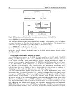
3.1.1 Asymptotic notation
In the asymptotic analysis of capacity of wireless network, the results are often presented
using the asymptotic notation (or big O-notation) (Bruijn, 2010). In this section we briefly
review the definition of some of the notation commonly used. In the following, we will
assume that f
(n) and g(n) are functions that map positive integers to positive real numbers.
Definition 1 We say that f
(n)=O(g(n)) (or, more precisely, f (n) ∈ O(g(n)), or even f (n) is
O
(g(n)))
1
, if there exists a constant c and there exists an integer n

0
≥ 1 such that f (n) ≤ cg(n) for
n
≥ n
0
(see Figure 1(a)).
In other words, f
(n)=O(g(n)) means that g(n) grows at least as fast as g(n ).
1
Formally, we should write f (n) ∈ O(g(n)), and the form f (n)=O(g(n)) is considered an abuse of
notation. In fact, the symmetry that the equals sign implicitly suggests does not exist in the statements
involving asymptotic notation.
457
A Survey on The Characterization of the Capacity of Ad Hoc Wireless Networks
6 Theor y and Applications of Ad Hoc Networks
n
o()
O()
f(n)
Ω()
n
n
0
f(n)
c
2
g(n)
c
1
g(n)

(a) (b)
Fig. 1. (a) Interpretation of O(), o() and Ω(); (b) Interpretation of f (n)=Θ(g(n)).
Definition 2 We say that f
(n)=o(g(n)) if for any positive constant c, there exists an integer n
0
≥1
such that f
(n) ≤cg(n) for n ≥n
0
(see Figure 1(a)).
The difference between the definitions of O
() and o() is that in the former there must exist
at least one constant c such that f
(n) ≤ cg(n), while in the latter the relation f (n) ≤ cg(n)
must be true for any constant c. Therefore, O() and o() provide tight and loose upper bounds,
respectively.
Definition 3 We say that f
(n)=Ω(g(n)) if there exists a constant c and there exists an integer
n
0
≥ 1 such that f (n) ≥ cg(n) for n ≥n
0
(see Figure 1(a)).
Definition 4 We say that f
(n)=Θ(g(n)) if there exist positive constants c
1
and c
2
, and there exists
n

0
≥ 1 such that c
1
g(n) ≤ f (n) ≤ c
2
g(n), for n ≥ n
0
. Equivalently, f (n )=Θ(g(n)) if f (n)=
O(g(n)) and f (n)=Ω(g(n)) (see Figure 1(b)).
Note that f
(n)=Θ(g(n)) means that g(n) is both a tight upper bound and a tight lower bound
on f
(n).
3.1.2 Capacity metrics
Definition 5 (Transport capacity) Let us suppose that node i successfully transmits to node j at
rate λ
ij
bits per second, and that the distance between i and j is d
ij
meters. Therefore, we can say that
the network transports λ
ij
× d
ij
bit·meter per second. Note that this metric expresses the difficulty of
transmitting to a longer distances. Transport Capacity T of a network is evaluates as
∑
i=j
λ
ij

d
ij
, where
λ
ij
is the feasible rate between nodes i and j.
Definition 6 (Throughput capacity) It is the guaranteed rate, measured in bits per second, that can
be supported uniformly for all source-destination pairs.
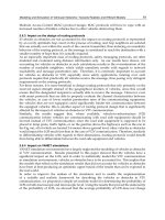
3.1.3 Interference models
Definition 7 (The protocol interference model) Let {(X
i
, X
R(i)
) : k ∈T}be the set of active
transmitter-receiver pairs in the network. According to the protocol interference model, this
transmission is successfully received if the distance between nodes X
R(i)
(the intended receiver of node
458
Mobile Ad-Hoc Networks: Applications
A Survey on the Characterization of the Capacity of Ad Hoc Wireless Networks 7
(a)
X
i
X
R(i)
(1+Δ)|X
i
- X
R(i)

|
RX
TX
X
k
Interferer
No interferer is allowed inside for
successful reception at X
R(i)
X
i
X
k
X
R(k)
(b)
|X
k
- X
R(k)
|
Δ
2
Exclusion
regions
X
R(i)
Fig. 2. The protocol model: (a) Disk around receiver X
R(i)
must be free of interfering nodes

for correct reception at node X
R(i)
; (b) Two links are successful if the corresponding exclusion
regions are disjoint.
X
i
transmission) and any other node X
k
transmitting on the same channel is larger than the distance
between X
i
and X
R(i)
, that is
|X
k
− X
R(i)
|≤(1 + Δ)|X
i
− X
R(i)
|, (5)
where
|X
k
−X
R(i)
| indicates the distance between nodes X
i

and X
R(i)
, and Δ > 0 is the spatial
protection margin. Figure 2(a) shows a geometric interpretation of this model. Now, let us
consider two pairs of active nodes X
i
and X
k
, with X
i
transmitting to X
R(i)
and X
k
transmitting
to X
R(k)
, and with both pairs operating under the protocol model, represented by expression
(5). We can show that, in order to have both transmissions successfully received, we must
have
|X
R(k)
− X
R(i)
|≥
Δ
2

|X
k

− X
R(k)
|+ |X
i
− X
R(i)
|

.(6)
This result indicates that circular exclusion regions around the receivers X
R(j)
and X
R(k)
,of
radius Δ
|X
i
− X
R(i)
|/2 and Δ|X
k
− X
R(k)
|/2, respectively, are disjoint, as shown Figure 2(b).
Therefore, exclusion regions around receivers of each successful transmission are mutually
disjoint, and consume a portion of the network area.
Definition 8 (The physical interference model) Consider, as before, a set of active
transmitter-receiver pairs
{(X
i

, X
R(i)
) : i ∈N}, transmitting over the same channel, with a
transmit power assignment
{P
i
}. According to the physical interference model, the transmission
from node X
i
is successfully received by node X
R(i)
if the signal-to-interference plus noise ratio (SINR)
at X
R(i)
is equal to or larger than a given threshold β, that is
P
i
|X
i
−X
R(i)
|
η
σ
2
+
∑
k∈N,k=i
P
k

|X
k
−X
R(i)
|
η
≥ β, (7)
459
A Survey on The Characterization of the Capacity of Ad Hoc Wireless Networks
8 Theor y and Applications of Ad Hoc Networks
X
i
X
R(i)
|X
k
- X
R(k)
|
Δ
2
Network area
Fig. 3. Arbitrary network under the Protocol Interference model: successful links correspond
to disjoint disks.
where σ
2
is the additive noise power. The threshold β depends on transmission parameters,
such as modulation technique, error correcting coding and the minimum acceptable bit error
rate.
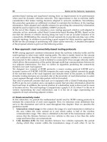
3.2 Transport capacity in arbitrary networks with immobile nodes

We consider in this section a network of n immobile nodes, which can act simultaneously as
source, relay or destination. These n nodes are arbitrarily located in a planar disk of unity area.
This means that the positions of the nodes can be adjusted in order to satisfy the conditions
for successful transmissions imposed by the interference model considered in the analysis.
Every node selects randomly another node as the destination of its bits. The results of this
analysis are presented in the sequel, for both the Protocol Interference model and the Physical
Interference model.
3.2.1 Capacity under the protocol interference model
The authors of (Gupta & Kumar, 2000) showed that the transport capacity T
A
of an arbitrary
network with n nodes under the Protocol Model is
T
A
= Θ(W
√
n) bit ·meter/s, (8)
This means that the transport capacity per node is Θ
(W
√
1/n) bit·meter/s, and goes to zero
as the number of nodes increases. Following (Xue & Kumar, 2006), this result can be proved
using the fact that, under the Protocol Interference model, disks of radius equals to Δ
|X
i
−
X
R(i)
|/2 centered at receiver nodes of successful links are disjoint (see Definition 7). Therefore,
each successful link consumes a fraction of the network area and the sum of the area of disks of

all successful links is upper limited by the network area (see Figure 3). Neglecting the border
effects (i.e., when nodes are close to the boundary of the network area), we can write
∑
i∈T (t)
π

Δ
2
d
i

2
≤ 1 →
∑
i∈T (t)
d
2
i
≤
4
πΔ
2
, (9)
where d
i
is the T-R separation distance |X
i
− X
R(i)
| of the i-th T-R pair, and T (t) is the set

of successful links at time t. This expression can be interpreted as follows: a set of n nodes
is accommodated in such way
2
that condition (9) is satisfied. It should be noted that, at any
2
Recall that we are dealing with the arbitrary network case.
460
Mobile Ad-Hoc Networks: Applications
A Survey on the Characterization of the Capacity of Ad Hoc Wireless Networks 9
given time t, at most n/2 nodes will be transmitting (the other n/2 nodes will be receiving).
Now, we can use the Cauchy-Schwarz inequality to write
n/2
∑
i=1
d
2
i
n/2
∑
j=1
1
2
≥

n/2
∑
i=1
d
i
×1


2
,
or
n/2
∑
i=1
d
i
≤




n/2
∑
i=1
d
2
i
n
2
≤

2n
πΔ
2
.
Therefore, we have found an upper bound on the sum of the T-R separation distances of
successful links. Now, if we assume that all sources transmit at rate W, then the transport

capacity T
A
of the network at a given time t is upper bounded as
T
A
= W
∑
i∈T (t)
d
i
≤

2
π
W
Δ
√
n,
or, T
A
= O(W
√
n) bit-meter/s. Now, we can also show that a transport capacity of
W
√
A
1+2Δ
n
√
n+

√
8π
bit-meter/s is achievable under the Protocol Interference Model (see (Xue &
Kumar, 2006) for details), completing the proof of (8).
Recalling that the network has n nodes, we can conclude that the transport capacity per node is
Θ
(W/
√
n). This means that the transport capacity diminishes to zero as the number of users
in the network increases. Note that we are assuming here that sources randomly select other
nodes as their destinations and, therefore, the average source-destination separation distance
does not depend on the number of nodes n. So, as n increases, we have more and more
nodes willing to send their bits over paths with the same average length, but sharing the same
available bandwidth.
3.2.2 Capacity under the physical interference model
Now, if the Physical Interference model is adopted, Kumar and Gupta (Gupta & Kumar, 2000)
showed that the transport capacity is
T
A
= O(Wn
α−1
α
) bit ·meter/s. (10)
This upper bound can be proved recalling that, according to the Physical Interference model,
a successful transmission requires that
P
i
d
−α
i

N +
∑
j∈T ,j=i
P
j
d
−α
j
≥ β. (11)
If we include the desired signal power in the summation in denominator, and isolate the term
d
α
i
,weget
d
α
i
≤
(
β + 1
)
P
i
β

N +
∑
j∈T
P
j

d
−α
j

. (12)
461
A Survey on The Characterization of the Capacity of Ad Hoc Wireless Networks
10 Theor y and Applications of Ad Hoc Networks
Noting that the T-R separation distance d
i
is smaller than the diameter of the network area,
i.e., d
i
≤ 2/
√
π, then
d
α
i
≤
(
β + 1
)
P
i
β

N +

π

4

α/2
∑
j∈T
P
j

≤
(
β + 1
)
P
i
β


π
4

α/2
∑
j∈T
P
j

. (13)
Now, summing the quantities d
α
i

of all active links, we get
∑
i∈T
d
α
i
≤
(
β + 1
)
β

4
π

α/2
. (14)
Next, we use the Holder’s inequality, according to which, for a, b
> 0, p, q ≥1 and 1/p + 1/q =
1,
∑
ab ≤

∑
a
p

1/p

∑

b
q

1/q
. (15)
Therefore, recalling that there are at most n/2 links, then
∑
i∈T
d
i
≤

∑
i∈T
d
α
i

1/α

∑
i∈T
1
α−1
α

α−1
α
≤


∑
i∈T
d
α
i

1/α

n
2

α−1
α
≤

(
β + 1
)
β

4
π

α/2

1/α

n
2


α−1
α
≤
1
√
π

2β
+ 2
β

1/α
n
α−1
α
. (16)
Finally, if all sources transmit at rate W, the transport capacity is upper bounded as
T
A
= W
∑
i∈T
d
i
≤
W
√
π

2β

+ 2
β

1/α
n
α−1
α
. (17)
Note that if capacity is equitably shared among all sources, the transport capacity per node is
T
A
= O(W/n
1/α
), and goes to zero as n increases. Note also that this bound indicates that a
larger path loss exponent α leads to a higher capacity. This can be explained by noting that
larger α means stronger signal attenuation and, therefore, reduced interference. Consequently,
concurrent links can be packed together, increasing capacity.
3.3 Throughput capacity in random networks with immobile nodes
3.3.1 Capacity under the protocol interference model
Gupta and Kumar also showed that the throughput capacity in bits per second of a random
network under the Protocol Model is upper bounded by
λ
(n) ≤
cW

nlogn
. (18)
This result can be proved using again the argument that successful transmissions consume
portions of the network area. Let us consider a network with n nodes randomly placed on a
462

Mobile Ad-Hoc Networks: Applications
A Survey on the Characterization of the Capacity of Ad Hoc Wireless Networks 11
(a) (b)
Network of unity
area with n nodes
Source Destination
L
r
n
r
n
Δ
2
Fig. 4. The protocol model: (a) Disks around active receivers must be disjoint; (b) Average
number of hops between source and destination.
disk of unity area. Let us also assume that all nodes transmit with a common transmission
range r
n
. In order to guarantee that no node is isolated in the network, it can be shown that
r
n
must be asymptotically larger than

logn/πn (Gupta & Kumar, 1998) (Penrose, 1997).
Next, we recall that, under the Protocol Interference model, successful transmissions require
that disks of radius Δr
n
/2, centered at receivers, must be disjoint, as shown in Figure 4(a).
Therefore, the number of successful transmissions N
S

within a disk of unity area is upper
bounded as
N
S
<
4
πΔ
2
r
2
n
. (19)
Therefore, the aggregate number of bits transmitted per second in the network cannot be
larger than
4W
πΔ
2
r
2
n
,
where W is the common transmission rate of the individual transmissions.
Now, as before, let us consider that source nodes choose at random their destination nodes,
and denote
L the average source-destination separation distance. Note that L does not depend
on the number of nodes in the network. Therefore, the average number of hops between
source and destination is lower bounded by
L/r
n
(see Figure 4(b)). If each source generates

bits at rate λ
(n), then the average number of bits transmitted by the whole network is given
by nλ
(n)L/r
n
and must satisfy
nλ
(n)
L
r
n
≤
4W
πΔ
2
r
2
n
. (20)
Finally, using r
n
>

logn/πn, we complete the proof of (18).
In this same context, i.e., random networks under the Protocol Interference model, Xue and
Gupta presented in (Xue & Kumar, 2006) a transmission scheme that achieves a throughput
λ
(n) ≤
cW
(

1 + Δ
)
2

nlogn
. (21)
To demonstrate that (21) is valid, n nodes are randomly placed in a square of unity area.
This area is tessellated by cells of side s
n
=

K log n/n, as shown in Figure 5(a). We can
463
A Survey on The Characterization of the Capacity of Ad Hoc Wireless Networks
12 Theor y and Applications of Ad Hoc Networks
(a) (b)
M cells
M
s
n
Fig. 5. The protocol model: (a) Tessellation of the unity square by cells of side s
n
, with
adjacent cells grouped in groups of M
2
cells (M = 4). Cells in blue are allowed to transmit
concurrently; (b) Source-destination lines crossing a given cell (adapted from (El Gamal et al.,
2006), copyright
c
2006 IEEE).

show that, with probability approaching one, each cell has at least one but no more than
Kelog n nodes (see (Xue & Kumar, 2006) for details). We suppose that nodes transmit with
a common transmission range such that every node can transmit to any node located in its
neighboring cells. In order to guarantee successful transmissions, by controlling interference,
the following transmission scheme is used. We divide the cells into groups of M
2
adjacent
cells (see Figure 5(a)). At each time-slot, one node from one cell of each group is allowed
to transmit. Therefore, at each time-slot, there will be n/M
2
concurrent transmissions (or
concurrent cells), as exemplified in Figure 5(b). Clearly, time is split into M
2
time-slots.
Successful transmissions are guaranteed if concurrent cells are enough far apart, being the
distance between concurrent cell controlled by the number M. Note that the required value
of M for successful transmission does not depend on n, as only one node from each cell
transmits at each time-slot. Therefore, under the Protocol Interference model, we can simply
set M
= c(1 + Δ) (Xue & Kumar, 2006). Since, as before, each source node chooses at random
its destination node, bits reach their destination by means of multi-hop routes. Therefore,
every node transmits not only its own bits, but also bits from other nodes. Therefore, the
number of bits each node pumps to the network (its own bits and those from other nodes) is
related to the number N
R
of multi hop routes crossing the cell to which the node belongs (see
Figure 5(b)). This number N
R
, in turn, is related to the number of lines connecting a source
and a destination that intersect a given cell. Xue and Gupta (Xue & Kumar, 2006) showed that,

with probability approaching one, N
R
≤ c

nlogn. Therefore, the number of bits transmitted
per second from a given cell is λ
(n)c


nlogn, where λ(n) is the throughput per node. If W is
the transmission rate in each time-slot, and recalling that there are
[
c(1 + Δ)
]
2
time-slots, then
each cell transmits at rate W/
[
c(1 + Δ)
]
2
. Therefore, the throughput per cell λ(n)c


nlogn is
feasible if
λ
(n)c



nlogn ≤
W
[
c(1 + Δ)
]
2
,
464
Mobile Ad-Hoc Networks: Applications
A Survey on the Characterization of the Capacity of Ad Hoc Wireless Networks 13
M cells
s
n
M
cells
Interfering
transmitters
X
i
X
R(i)
Fig. 6. Evaluation of the interference in a tesselated network under the Physical Interference
model.
concluding the proof of (21). It should be noted that one node in each cell can be designated
to handle all relay traffic, while all other nodes act as sources or destinations.
Note that while (18) gives an upper bound on the throughput per node, (21) gives a feasible
throughput, and we say that the order of the throughput of random networks under the Protocol
Interference model is
λ
(n)=Θ


W

nlogn

. (22)
As noted in (Xue & Kumar, 2006), the result in (22) suggests that the throughput of random
networks is almost that achieved in the best case scenario (arbitrary networks), in which
throughput is O
(1/
√
n), despite the fact that nodes are optimally located.
3.3.2 Capacity under the physical interference model
When the Physical Interference model is used, it can be shown that throughput per bits per
second
λ
(n)=Θ

W

nlogn

(23)
is feasible. This result can be derived using the same transmission scheme used in Section 3.3
.1. We just need to show that M can be selected such that transmissions can achieve SINR
≥ β ,
as required by the Physical Interference model for successful transmission (Xue & Kumar,
2006). In order to show that, let us consider the transmission from node X
i
to receiver X

R(i)
in a network tesselated as before, as shown in Figure 6. This transmission is disturbed by
transmissions from nodes located in the concurrent cells, which are arranged according to tiers
of 8k cells, with k
= 1, 2,···. Using simple geometric arguments, we see that in the worst-case
scenario, the distance between X
i
and X
R(i)
is 2
√
2s
n
, and the distances between receiver X
R(i)
and interferers of the k-th tier are larger than kMs
n
−2s
n
. The aggregate interference power
465
A Survey on The Characterization of the Capacity of Ad Hoc Wireless Networks
14 Theor y and Applications of Ad Hoc Networks
can therefore be upper bounded as
∑
k∈N,k=i
P
k
|X
k

− X
R(i)
|
α
≤
∞
∑
k=1
8k
P
(
kMs
n
−2s
n
)
α
≤
8P
(Ms
n
)
α
∞
∑
k=1
k
(
k −2/M
)

α
.
It can be shown that
∑
∞
k
=1
k
(
k−2/M
)
α
converges when α > 2 (Xue & Kumar, 2006), and therefore
there is a value of M sufficiently large that guarantees SINR
≥ β at the receiver. Therefore,
the throughput
λ
(n)=
cW

nlogn
is feasible in a random network under the Physical Interference model as well.
An upper bound on the throughput for random network under the Physical Interference
model can be derived using the upper bound on the throughput for the case under the
Protocol Interference model. In fact, successful links
(X
i
, X
R(i)
) in a random network under

the Physical Interference mode are also successful under the Protocol Model, for appropriate
values of Δ and β. Therefore, an upper bound on the throughput for the Protocol Model also
holds for the Physical Interference model. Therefore, for a random network under the Physical
Interference model the throughput is upper bounded as
λ
(n) <
cW
√
n
. (24)
3.4 Capacity with directional antennas
In the previous sections we assumed that transmitters and receivers are equipped with
omnidirectional antennas. However, it is well known that directional antennas can reduce
interference and, consequently, increase capacity. Yi et al. (Yi et al., 2007) extended the work
done by Gupta and Kumar by including directional antennas in the model, and investigated
the effects of directional antennas on the capacity scaling laws. The radiation pattern adopted
by Yi et al. is modeled as a sector with beamwidth α, for the transmit antenna, and β, for
the receive antenna. This is a rather optimistic model as it assumes that the energy irradiated
outside the main bean is zero (i.e., sidelobes have zero gain). Following the same reasoning as
in (Gupta & Kumar, 2000), the authors in (Yi et al., 2007) show that the throughput capacity
per node for a arbitrary network under the Protocol Interference model scales as
λ
(n)=O

1

nαβ

. (25)
Therefore, capacity increases as beamwidth decreases, what can be explaining by the fact that

directional antennas reduces the overall interference, and more concurrent transmissions can
be accommodated at a given time. However, even though the use of directional antennas may
increase capacity, it does not change the form of the scaling law of capacity. That would be
possible if α and β decreased as fast as 1/
√
n, leading to a constant throughput per node as
the size n of the network increases.
Spyropoulos and Raghavendra (Spyropoulos & Raghavendra, 2003) also investigated the
effects of directional antennas on the capacity scaling laws of ad hoc networks, but using more
466
Mobile Ad-Hoc Networks: Applications
A Survey on the Characterization of the Capacity of Ad Hoc Wireless Networks 15
(b)
θ
G
side
θ
R
2
R
1
(a)
Node A
Exclusion region
of node A
Fig. 7. (a) Idealized radiation pattern; (b) Exclusion region created when the Protocol
Interference model is used with the radiation pattern in (a): for successful reception at node
A, no other receiver can be located inside such exclusion region.
general antenna models. First, they considered an idealized radiation pattern with beamwidth
θ with unity gain, and constant sidelobe with gain G

side
< 1, as shown in Figure 7(a). When
this radiation pattern is assumed at both transmitters and receivers, the use of the Protocol
Interference model results in an exclusion region as shown in Figure 7(b), in which R
1
and R
2
are given by
R
1
=
[(
P/P
th
)
G
side
]
1/α
and R
2
=

(
P/P
th
)
G
2
side


1/α
. (26)
Therefore, small gain G
side
leads to small exclusion area, which, in turn, leads to a large
number of concurrent transmissions. In fact, Spyropoulos and Raghavendra showed that the
throughput capacity per node is upper bounded as
λ
(n) ≤
cW

nlogn
1
θG
side
+(2π − θ)G
2
side
. (27)
In the directional antenna model adopted by Spyropoulos and Raghavendra, a narrow beam
is steered towards the intended node, and out of the main beam, the antenna gain is constant.
This, however, is not an appropriate model for the so called smart antenna, which are capable of
not only steering a narrow beam towards a given direction, by also steering strong attenuation
(nulls) towards some directions, in order to mitigate the signal from known interfering
transmitters. In order to evaluate the effects of a smart antenna on the network capacity,
Spyropoulos and Raghavendra considered that a smart antenna with N elements can steer a
beam of gain G
max
= 1 towards the desired direction, and gains G

null
 1 towards at most
N
− 2 different directions. Now, the use of this antenna model together with the Protocol
Interference model allows for the accommodation of at most N
−2 receiving nodes within a
circle of radius R
=
(
P/P
th
)
1/α
, and the throughput capacity per bits/sec per node is upper
bounded as
λ
(n) ≤
cW(N −2)

nlogn
. (28)
467
A Survey on The Characterization of the Capacity of Ad Hoc Wireless Networks
16 Theor y and Applications of Ad Hoc Networks
(a) (b)
Destination
Destination
Relay
Source
Source

Phase 1 Phase 2
Fig. 8. The 2-hop relaying transmission scheme adopted by Tse and Grossglauser: (a) In
Phase 1, source transmits its packet to a relay node within its transmission range; (b) in Phase
2, packet is sent to the destination when the relay node gets close enough to the destination
node (adapted from (Grossglauser & Tse, 2002), copyright
c
2002 IEEE).
3.5 Networks with mobile nodes
Grossglauser and Tse (Grossglauser & Tse, 2002) extended in another direction the work done
by Gupta and Kumar, by introducing mobility in the model. As discussed in previous sections,
throughput in a network with immobile nodes decays as 1/
√
n due to the traffic increase
caused by multi hop connections between sources and destinations. Alternatively, one could
use large transmission ranges in order to reduce the number of hops between source and
destination. However, this strategy limits the number of concurrent transmissions, limiting
the capacity of the network. Other alternative would be to restrict transmissions to neighbors.
However, only a small fraction of sources are close enough to their destination nodes, limiting
capacity as well. In the light of this observation, and considering a network of mobile nodes,
Grossglauser and Tse (Grossglauser & Tse, 2002) developed a 2-hop relaying transmission
scheme with two phases, described in the following as exemplificed in Figure 8:
– Phase 1: A packet generated by a node is either directly transmitted to the corresponding
destination node, or relayed to a intermediate (relay) node. In the former case, the
transmission session is concluded.
– Phase 2: If the packet is sent to a relay node, the packet is buffered until the relay node
is close enough to the destination node, when the packet is eventually sent to its final
destination.
Note that an essential aspect of this scheme is that , due to mobility, the relay node and
the destination nodes will eventually be close enough to each other to allow communication
between them. Based on this model, Grossglauser an Tse showed that the average long-term

throughput per S-D pair remains constant as n increases, that is, throughput scales as Θ
(1).
An important aspect of this analysis is that the mobility model adopted assumes that, at a
given time, a node is equally likely to be in any part of the network, meaning that the network
topology completely changes over time. Clearly, this mobility model is an oversimplification
of a real scenario, but the results obtained under this model can be viewed as upper bound on
the performance.
468
Mobile Ad-Hoc Networks: Applications
A Survey on the Characterization of the Capacity of Ad Hoc Wireless Networks 17
Grossglaucer and Tse pointed out that throughput remains constant as n increases at the
expenses of an increasing delay. This has motivated several studies of the tradeoff between
delay and throughput in ad hoc networks (El Gamal et al., 2006), (Herdtner & Chong, 2005),
(Lin et al., 2006), (Neely & Modiano, 2005), (Sharma et al., 2007). For instance, El Gamal et.
al (El Gamal et al., 2006) investigated this tradeoff not only for mobile networks, but also for
static networks. For mobile networks, they considered a network operating under the same
2-hop relaying transmission scheme adopted by Grossglauser an Tse, and assumed a mobility
model named random-walk model, according to which nodes move a distance 1/
√
n per
unit time. They then showed that the throughput scales as Θ
(1), as in (Grossglauser & Tse,
2002), but the delay scales as Θ
(n log n). For static network, El Gamal et. al showed that, at
throughput Θ
(1/

nlogn) (as in the work done by Gupta and Kumar), the average delay is
Θ
(


n/ log n) .
Another important extension of the work done by Grossglaucer and Tse is the one carried
out by Herdtner and Chong (Herdtner & Chong, 2005) in which the authors showed that
mobility alone does not increase capacity of ad hoc networks. Specifically, they showed that
if the buffer size of nodes is finite and limited to Θ
(1), i.e., it remains constant as n increase,
then the throughput capacity is only O
(1/
√
n), instead of Θ(1). Therefore, a scaling law for
throughput in a mobile network in the form Θ
(1) is only possible if the buffer size increases
as n increases.
Lin et al. (Lin et al., 2006) investigated the tradeoff between capacity and delay in a mobile
wireless network, assuming a Brownian motion model. A key parameter in this mobility
model is the variance σ
2
, which is related to the time required by a node to move to different
parts of the network. Large σ
2
means that the node will take a short amount of time to
move. The authors of (Lin et al., 2006) showed that, under the 2-hop relaying transmission
scheme proposed by Grossgluaser and Tse, throughput of Θ
(1) is achieved at the expenses of
an average delay of Ω
(log n/σ
2
), showing how the node speed affects the delay.
4. Summary

This chapter provided an overview of metrics for capacity evaluation of ad hoc wireless
networks. The peculiarities of wireless ad hoc networks make the estimation of capacity of
this kind of networks a complex task, which is evidenced by the variety of capacity metrics
found in the literature.
The capacity metrics discussed in this chapter can be classified into two groups: metrics
based on a statistical approach, and metrics focused on the network scalability. In the first
group, discussed in Section 2, capacity metrics incorporate aspect from the physical layer (e.g.
modulation parameters, spectral efficiency, etc.) and from the network layer (e.g. spatial
reuse, number of hops, etc.). Therefore, these metrics are suitable for network design and
parameter optimization.
The metrics in the second group, discussed in Section 3, essentially describe how network
capacity behaves when the number of nodes in the network grows. As can be noted from the
discussion presented in Section 3, the scaling laws derived are closely related to the particular
network model and transmission scheme assumed. Therefore, even though the resulting
scaling laws are rather pessimistic (per-node capacity vanishes as the size of the network
increases), the results can be used as guideline for the design of more appropriate transmission
schemes, that would hopefully result in non-vanishing capacity.
469
A Survey on The Characterization of the Capacity of Ad Hoc Wireless Networks
18 Theor y and Applications of Ad Hoc Networks
5. References
Andrews, J., Shakkottai, S., Heath, R., Jindal, N., Haenggi, M., Berry, R., Guo, D., Neely, M.,
Weber, S., Jafar, S. & Yener, A. (2008). Rethinking information theory for mobile ad
hoc networks, IEEE Communications Magazine 46(12): 94–101.
Baddeley, A. (2007). Spatial point processes and their applications, Stochastic Geometry,
Springer, pp. 1–75.
Bruijn, N. (2010). Asymptotic Methods in Analysis, Dover Publications.
Chandra, M. & Hughes, B. (2003). Optimizing information efficiency in a direct-sequence
mobile packet radio network, Communications, IEEE Transactions on 51(1): 22–24.
URL: 10.1109/TCOMM.2002.807607

El Gamal, A., Mammen, J., Prabhakar, B. & Shah, D. (2006). Optimal throughput-delay scaling
in wireless networks - part i: the fluid model, Information Theory, IEEE Transactions on
52(6): 2568 –2592.
Grossglauser, M. & Tse, D. (2002). Mobility increases the capacity of ad hoc wireless networks,
Networking, IEEE/ACM Transactions on 10(4): 477–486.
URL: 10.1109/TNET.2002.801403
Gupta, P. & Kumar, P. (2000). The capacity of wireless networks, IEEE Trans. on Information
Theory 46(2): 388–404.
Gupta, P. & Kumar, P. R. (1998). Stochastic Analysis, Control, Optimization and Applications: A
Volume in Honor of W.H. Fleming, Birkhauser, chapter Critical power for asymptotic
connectivity in wireless networks, pp. 547 – 560.
Herdtner, J. & Chong, E. (2005). Throughput-storage tradeoff in ad hoc networks, INFOCOM
2005. 24th Annual Joint Conference of the IEEE Computer and Communications Societies.
Proceedings IEEE, Vol. 4, pp. 2536 – 2542 vol. 4.
Jindal, N., Weber, S. & Andrews, J. (2008). Fractional power control for decentralized wireless
networks, IEEE Trans. on Wireless Communications 7(12): 5482–5492.
Kaynia, M., Nardelli, P., Cardieri, P. & Latva-aho, M. (2010). On the optimal design of MAC
protocols in multi-hop ad hoc networks, Sixth Workshop on Spatial Stochastic Models
for Wireless Networks.
Kleinrock, L. & Silvester, J. (1978). Optimum transmission radii for packet radio networks or
why six is a magic number, National Telecommunications Conference.
Liang, P. & Stark, W. (2000). Transmission range control and information efficiency for
FH packet radio networks, MILCOM 2000. 21st Century Military Communications
Conference Proceedings, Vol. 2, pp. 861–865 vol.2.
URL: 10.1109/MILCOM.2000.904053
Lin, X., Sharma, G., Mazumdar, R. & Shroff, N. (2006). Degenerate delay-capacity tradeoffs
in ad-hoc networks with brownian mobility, Information Theory, IEEE Transactions on
52(6): 2777 –2784.
Mignaco, A. & Cardieri, P. (2006). Total information efficiency in multihop wireless networks,
IEEE International Performance, Computing, and Communications Conference.

Nardelli, P. & Cardieri, P. (2008a). Aggregate information efficiency and packet delay in
wireless ad hoc networks, IEEE Wireless Communications and Networking Conference.
Nardelli, P. & Cardieri, P. (2008b). Aggregate information efficiency in wireless ad hoc
networks with outage constraints, IEEE International Workshop on Signal Processing
Advances in Wireless Communications.
Nardelli, P., de Abreu, G. & Cardieri, P. (2009). Multi-hop aggregate information efficiency in
wireless ad hoc networks, Communications, 2009. ICC ’09. IEEE International Conference
470
Mobile Ad-Hoc Networks: Applications