Artificial Neural Networks Industrial and Control Engineering Applications Part 14 pdf

Artificial Neural Networks - Industrial and Control Engineering Applications

444

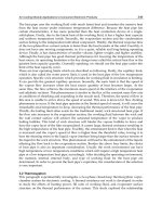
1. Air compressor
2. Service Unit
3. SPC 200 Controller
4. Analog Pressure Transducers
5. Gripper
6. Y axis
7. Linear Potentiometer for x axis
8. X axis
9. NI Compact FieldPoint System
10. Power Supply
Fig. 1. Servo-pneumatic positioning system of the Festo Didactic. The components of the
system are the following:
Experimental data was collected by using the National Instrument (NI) compact FieldPoint
measurement system with control modules. The LabVIEW program environment controlled
the measurement system. The values of four analog parameters were monitored. Three of
these parameters were the pressure readings of the cylinders creating the motion in the x
and y directions and the overall system. The Fourth analog input was the readings from the
linear potentiometer. The gripper action was monitored from the digital signals coming
from data acquisition card. The diagram of the components of the servo-pneumatic system
is shown in Figure 2.
Conditioning Monitoring and Fault Diagnosis for a
Servo-Pneumatic System with Artificial Neural Network Algorithms

445

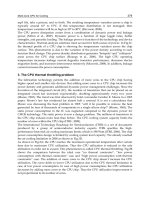
Fig. 2. The servo-pneumatic system components for X axis. (1. Measuring system, 2. Axis
interface, 3. Smart positioning controller SPC 200, 4. Proportional directional control valve,

5. Service unit, 6. Rodless cylinder) ((festodidactic.com, 2010)
The servo-pneumatic system simulated the operation of food preparation. Jars were put
individually on a conveyor belt by the packaging system. A handling device with servo-
pneumatic NC axis transferred these jars to a pallet. The precise motion of the NC axis is
essential for completion of the task (Festo Didactic, 2010).
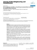
The user interface of the LabVIEW program is presented in Fig. 3. The display shows the
pressures of the overall system and two cylinders creating the motions along the X and Y
axes. Also the displacement of one of the cylinder and gripper action (pick and place) is
demonstrated.
In this study, the pneumatic system was operated at the normal and 4 different faulty
conditions. The experimental cases are listed in Table 1. There were 15 experimental cases.
The data was collected at the same condition 3 times when the system was operated in the
normal and 4 faulty modes.

Operational condition Experiment # Recalled as

Normal operation of the Servo Pneumatic System 1 Normal
x axis error positioning 2 Fault 1
y axis error positioning 3 Fault 2
Pick faults for gripper 4 Fault 3
Place faults for gripper 5 Fault 4
Table 1. Operating conditions
Artificial Neural Networks - Industrial and Control Engineering Applications

446

Fig. 3. Data collection visual front panel of LabVIEW
The signals of the gripper pick (Fig.4) and place (Fig.5) sensors, the pressure sensors of the
cylinders in the x (Fig.6) and y (Fig.7) directions, the voltage output of the linear
potentiometer of the x axis (Fig.8) are presented in the corresponding figures.

0 5 10 15
0
0.2
0.4
0.6
0.8
1
Time (s)
Gripper Position
Normal
Fault1
Fault2
Fault3
Fault4

Fig. 4. Gripper Pick
Conditioning Monitoring and Fault Diagnosis for a
Servo-Pneumatic System with Artificial Neural Network Algorithms

447


Sensor
0 5 10 15
0
0.2
0.4
0.6

0.8
1
Time (s)
Griper Position
Normal
Fault1
Fault2
Fault3
Fault4

Fig. 5. Gripper Place Sensor


0 5 10 15
1
1.5
2
2.5
3
Time (s)
Pressure of X Axis (bar)
Normal
Fault1
Fault2
Fault3
Fault4


Fig. 6. X Axis Pressure
Artificial Neural Networks - Industrial and Control Engineering Applications

448

Sensor
5 10 15
1
1.5
2
2.5
3
Time (s)
Pressure of Y Axis (bar)
Norma l
Fault1
Fault2
Fault3
Fault4

Fig. 7. Y Axis Pressure Sensor
5 10 15
0
1
2
3
4
5
6
7
8
9

10
Time
(
s
)
Linear Potentiometer
Normal
Fault1
Fault2
Fault3
Fault4

Fig. 8. X Axis linear potentiometer signal
4. Proposed encoding method
The sensors provided long data segments during the operation of the system. To represent
the characteristics of the system the sensory signals were encoded by selecting their most
descriptive futures and presented to the ANNs.
Conditioning Monitoring and Fault Diagnosis for a
Servo-Pneumatic System with Artificial Neural Network Algorithms

449
Two gripper sensor signals were monitored one for pick (Fig.4) and one for place (Fig.5).
Their outputs were either 0 V or 1V. The gripper pick and place signals were encoded by
identifying the time when the value raised to 1V and when it fell down to 0V. The signals of
the pressure of x axis (Fig.6), pressure of y axis (Fig.7) and main pressure were encoded by
calculating their averages. For the linear potentiometer (Fig.8) the times when the signal fell
below 7V and when it went over 7V were identified and used during the classification.
5. Results
The expected results from the ANN classification are presented in Fig.9. Ideally, once the
ANN experiences the normal and each faulty mode, someone may expect it to identify each

one of them accurately. In our case this means, an unsupervised ANN create maximum 5
categories and assign each one of them to the normal and 4 fault modes. Similarly, the
output of the supervised ANNs are supposed to be an integer value between 1 and 5
depending on the case. It is very difficult to classify the experimental data in 5 different
categories unless the encoded cases have very different characteristics, repeatability is very
high and noise is very low. In the worst case, we expect the ANN to assign at least two
categories and locate the normal operation and faulty ones in separate categories. The
output of the supervised ANN could be 0 and 1 in such cases. The ANN estimates in the
ideal and accdptialbe worst case scenario are demonstrated in Fig.9. In the following
sections, the performance of the supervised and the unsupervised ANNs are outlined.



0 5 10 15
1
1.5
2
2.5
3
3.5
4
4.5
5
Cases
Assigned category
Classification of the experimental data


Minimum
Best

Fig. 9. The output of the ANNs for classification of normal and 4 faulty modes.
Artificial Neural Networks - Industrial and Control Engineering Applications

450
5.2 Performance of the supervised ANNs:
Performance of the feed-forward-network (FFN) was evaluated by using the Levenberg
Marquardt algorithm. The FFN had 9 inputs and 1 output. The outputs of the cases were 1,
2, 3, 4, 5 for Normal, Fault1, Fault2, Fault3 and Fault4 respectively. For training only one
sample of the normal and 4 faulty cases were used. Since the FNN type ANNs do not have
any parameters to adjust their sensitivity they have to be trained with very large number of
cases which will teach the network expected response for each possible situation. Since, one
sample for each one of the normal and 4 faulty cases was too few for effective training, we
generated semi experimental cases. The semi-experimental cases were generated from these
samples by changing the each input with ±1% steps up to ±10%. We generated 100 semi-
experimental cases in addition to the original 5 cases with this approach. The FNN had 8
neurons at the hidden layer. The FFN was trained with 105 cases.
The FFN type ANN was trained by using the Levenberg-Marquardt algorithm of the Neural
Network Toolbox of the MATLAB. The training was repeated several times. The same semi-
experimental data generation procedure was used to generate 200 additional test cases from
the 10 experimental cases which had 2 tests at each condition (1 normal and 4 faulty ones).
The average estimation errors were 5.55e-15% for the training and 8.66% for the test cases.
The actual and estimated values for the training and test cases are presented in Fig.10 and
Fig.11 respectively. The ANN always estimated the training cases with better than 0.01%
accuracy. The accuracy of the estimations of the test cases was different at each trail. These
results indicated that, without studying the characteristics of the sensory signals very

0 20 40 60 80 100 120
0.5

1
1.5
2
2.5
3
3.5
4
4.5
5
Case number
Category
Performance of the Levenberg-Marquardt algorithm (Training cases)


Actual
Estimation

Fig. 10. The FFN type ANN estimations for the training cases.
Conditioning Monitoring and Fault Diagnosis for a
Servo-Pneumatic System with Artificial Neural Network Algorithms

451


0 50 100 150 200 250
0.5
1
1.5
2
2.5

3
3.5
4
4.5
5
Case number
Category
Performance of the Levenberg-Marquardt algorithm (Test cases)


Actual
Estimation



Fig. 11. The FFN type ANN estimations for the test cases.
carefully, the ANN may estimate the normal and faulty cases; however, for industrial
applications the characteristics of the data may change in much larger range than ours and
working with much larger experimental samples are advised.
The same analysis was repeated by using the fuzzy ARTMAP. The fuzzy ARTMAP adjusts
the size of the “category boxes” according to the selected vigilance value. The ANN
estimates the category of the given case as -1 if the fuzzy ARTMAP do not have proper
training. So, we did not need to use the semi-experimental data. The fuzzy ARTMAP was
trained by using 5 cases (normal and 4 fault modes). It was tested by using the 10 cases (2
normal and 8 faulty cases (2 samples at each fault modes)). The vigilance was changed from
0.52 to 1 with the steps of 0.02. The identical performance was observed for the training and
test cases when the vigilance was selected between 0.52 and 0.83 (Fig.12). All the training
cases were identified perfectly. The normal and all the faulty ones were distinguished
accurately. The fuzzy ARTMAP only confused two test cases belong to Fault 2 and 3. The
performance of the fuzzy ARTMAP started to deteriorate at the higher vigilances since the

“category boxes” were too small and the ANN could not classify some of the test cases. The
number of the unclassified cases increased with the increasing vigilance.
Artificial Neural Networks - Industrial and Control Engineering Applications

452


1 1.5 2 2.5 3 3.5 4 4.5 5
1
2
3
4
5
Cases
Category
Fuzzy ARTMAP - Training Cases Vigilance=0.52
1 2 3 4 5 6 7 8 9 10
1
2
3
4
5
Cases
Category
Fuzzy ARTMAP - Test Cases Vigilance=0.52


Fig. 12. The performance of the fuzzy ARTMAP type ANN.
5.1 Performance of the unsupervised ANNs:
Performance of the ART2 is shown in Table 2. It distinguished the normal and faulty cases.

Among the faults, the Fault 3 was identified all the time by assigning a new category and
always estimating it accurately. The ART2 could not distinguish Fault 1, 2 and 4 from each
other. The best vigilance values were in the range of 0.9 and 0.9975. When these vigilances
were used ART2 distinguished the normal operation, faulty cases and Fault 3. The same
results are also presented with a 3D graph in Fig.13.
The results of the Fuzzy ART program are presented in Fig.14. The number of assigned
categories varied between 2 and 15 for the vigilance values of 0.5 and 1. When the
vigilance was 0.5, the Fuzzy ART distinguished the normal and faulty operation but could
not classify the faults. Fuzzy ART started to distinguish Fault 4 when the vigilance was
0.65. It started to distinguish Fault 3 and 4 for the vigilance value of 0.77. When the
vigilance reached to 0.96 it could distinguished 10 categories and classified all the cases
accurately. Multiple categories were assigned to the normal and some of the faulty
operation modes.
Conditioning Monitoring and Fault Diagnosis for a
Servo-Pneumatic System with Artificial Neural Network Algorithms

453
Vigilance values
Condition
of the
system
Experiment
0.9 -
0.9975
0.998 0.9985 0.999 0.9995
Test 1 1 1 1 1 1
Test 2 1 2 2 2 2
Normal
Test 3 1 2 2 2 2
Test 1 2 3 3 3 3

Test 2 2 3 3 3 4
Fault 1
Test 3 2 3 3 3 4
Test 1 2 3 3 3 4
Test 2 2 3 3 3 4
Fault 2
Test 3 2 3 3 3 5
Test 1 3 4 4 4 6
Test 2 3 4 4 4 6
Fault 3
Test 3 3 4 4 4 6
Test 1 2 3 3 3 5
Test 2 2 3 3 3 5
Fault 4
Test 3 2 3 3 3 7
Table 2. The estimated categories with the ART 2 algorithm

0.9975
0.998
0.9985
0.999
0.9995
1
0
5
10
15
1
2
3

4
5
6
7
Vigilance
ART2 - Number of Categories at different vigilances
Cases
Assigned category

Fig. 13. The graphical presentation of the ART2 results in the Table 1.
Artificial Neural Networks - Industrial and Control Engineering Applications

454

0.5
0.6
0.7
0.8
0.9
1
0
5
10
15
0
5
10
15
Vigilance
Fuzzy ART - Number of Categories at different vigilances

Cases
Assigned category

Fig. 13. The estimations of the Fuzzy ART
6. Conclusion
A two axis servopneumatic system was prepared to duplicate their typical operation at the
food industry. The system was operated at the normal and 4 faulty modes. The
characteristics of the signals were reasonably repetitive in each case. Three pressure, one
linear displacement and two digital signals from the gripper were monitored in the time
domain. The signals were encoded to obtain their most descriptive futures. There were 15
experimental cases. The data was collected at the same condition 3 times when the system
was operated in the normal and 4 faulty modes. The encoded data had 9 parameters. The
performances of two supervised and two unsupervised neural networks were studied.
The 5 experimental cases were increased to 105 by generating semi experimental data. The
parameters of the FFN was calculated by using the Levenberg-Marquardt algorithm. The
average estimation errors were 5.55e-15% for the training and 8.66% for the test cases. The
fuzzy ARTMAP was trained with 5 cases including one normal and 4 faulty modes. It
estimated the 8 of the 10 test cases it never saw before perfectly. It confused the two faulty
cases among each other.
The ART2 and fuzzy ART were used to evaluate the performance of these unsupervised
ANNs on our data. Both of them distinguished the normal and faulty cases by assigning
different categories for them. They had hard time to distinguish the faulty modes from each
Conditioning Monitoring and Fault Diagnosis for a
Servo-Pneumatic System with Artificial Neural Network Algorithms

455
other. Since they did not need training, they are very convenient for industrial applications.
However, it is unrealistic to expect them to assign different categories for the normal
operation and each fault modes, and classify all the incoming cases accurately.
7. References

Aykut, S., Demetgul, M. & Tansel, I. N. (2010). Selection of Optimum Cutting Condition of
Cobalt Based Alloy with GONN. The International Journal of Advanced Manufacturing
Technology, Vol. 46, No. 9-12, pp. 957-967.
Beale, M. H., Hagan, M. T. & Demuth, H. B. (2010). Neural Network Toolbox 7 User Guide,
Mathworks.

Belforte, G., Mauro, S. & Mattiazzo, G. (2004). A method for increasing the dynamic
performance of pneumatic servo systems with digital valves, Mechatronics, Vol.14,
pp. 1105–1120.
Bryson, A. E., Ho, Y. C. (1975). Applied optimal control: optimization, estimation, and
control. Taylor & Francis Publishing, pp. 481.
Bouamama, B.O. et al. (2005). Fault detection and isolation of smart actuators using bond
graphs and external models, Control Engineering Practice, Vol. 13, pp.159-175.
Carpenter, G. A & Grossberg, S. (1987). ART-2: Self-Organization of Stable
Category Recognition Codes for Analog Input Pattern, Applied Optics, Vol. 26, pp.
4919-4930.
Carpenter, G. A., Grossberg S., & Reynolds J. H. (1991). ARTMAP: Supervised real-time
learning and classification of nonstationary data by a self-organizing neural
network, Neural Networks , Vol. 4, pp.565-588.
Carpenter, G. A., Grossberg, S. & Rosen, D. B. (1991a). ART 2-A: An adaptive resonance
algorithm for rapid category learning and recognition, Neural Networks , Vol. 4, pp.
493-504.
Carpenter, G. A., Grossberg, S. & Rosen, D. B. (1991b). Fuzzy ART: Fast stable learning
and categorization of analog patterns by an adaptive resonance system,
Neural Networks , Vol. 4, pp. 759-771.
Carpenter, G. A. et al. (1992). Fuzzy ARTMAP: A neural network architecture for
incremental supervised learning of analog multidimensional maps, IEEE
Transactions on Neural Networks, Vol. 3, pp. 698-713.
Chen, C. & Mo, C. (2004). A method for intelligent fault diagnosis of rotating machinery,
Digital Signal Processing, Vol. 14, pp. 203–217.

Chena, P. et al. (2007). A study of hydraulic seal integrity. Mechanical Systems and Signal
Processing, Vol. 21, pp.1115-1126.
Demetgul M.; Tansel IN. & Taskin S. (2009). Fault Diagnosis of Pneumatic Systems with
Artificial Neural Network Algorithms. Expert Systems with Applications, Vol. 36, No.
7, pp. 10512-10519.
Festo Didactic GmbH & Co. PneuPos Manuel, 2010.
/>4.pdf.
Garrett, A. (2003). Fuzzy ART and Fuzzy ARTMAP Neural Networks,
Artificial Neural Networks - Industrial and Control Engineering Applications

456

Gary M. & Ning, S., (2007). Experimental Comparison of Position Tracking Control
Algorithms for Pneumatic Cylinder Actuators, IEEE/ASME Transactions on
Mechatronics, October 2007.
Grossberg S. (1987). Competitive learning: From interactive activation to adaptive
resonance, Cognitive Science, Vol. 11, pp. 23-63.
Huang, R.; Xi, L.; Li, X.; Liu, C.R.; Qiu, H. & Lee, J. (2007). Residual life predictions for ball
bearings based on self-organizing map and back propagation Neural network
methods, Mechanical Systems and Signal Processing, Vol. 21, pp.193–207.
Karpenko, M.; Sepehri, N. & Scuse, D. (2003). Diagnosis of process valve actuator faults
using a multilayer Neural network. Control Engineering Practice, Vol. 11, pp.1289-
1299.
Lee, I. S.; Kim, J. T.; Lee, J. W.; Lee, D. Y. & Kim, K. Y. (2003). Model-Based Fault Detection
and Isolation Method Using ART2 Neural Network, International Journal of
Intelligent Systems, Vol.18, pp. 1087–1100.
Li, X. & Kao, I. (2005). Analytical fault detection and diagnosis (FDD) for pneumatic systems
in robotics and manufacturing automation. Intelligent Robots and Systems,
IEEE/RSJ International Conference, pp.2517-2522.
Lu, P. J.; Hsu, T. C.; Zhang, M. C. & Zhang, J. (2000), An Evaluation of Engine Fault

Diagnostics Using Artificial Neural Networks, ASME J. Eng. Gas Turbines Power,
Vol. 123, pp. 240–246.
McGhee, J.; Henderson, I. A. & Baird, A. (1997). Neural networks applied for the
identification and fault diagnosis of process valves and actuators, Measurement, Vol.
20, No. 4, pp. 267-275.
Mendonça, L. F.; Sousa, J. M. C. & Costa, J. M. G. (2009). An architecture for fault detection
and isolation based on fuzzy methods, Expert Systems with Applications. Vol. 36 pp.
1092–1104.
Na, C. & Lizhuang, M. (2008). Pattern Recognition Based on Weighted and Supervised
ART2. International Conference on Intelligent System and Knowledge Engineering,
Xiamen, China, Nov. 17-18, 2008,Vol. 2, pp. 98-102.
Nakutis, Ž., Kaškonas, P. (2005). Application of ANN for pneumatic cylinder leakage
diagnostics. Matavimai, Vol. 36, No.4, pp.16-21.
Nakutis, Ž. & Kaškonas, P. (2007. Pneumatic cylinder diagnostics using classification
methods. Instrumentation and Measurement Technology Conference Proceedings,
Warsaw, 1-3 May 2007, pp.1-4.
Nakutis, Ž. & Kaškonas, P. (2008). An approach to pneumatic cylinder on-line conditions
monitoring. Mechanika. Kaunas: Technologija, Vol. 4, No. 72, pp.41-47.
Nazir, M. B. & Shaoping, W. (2009). Optimization Based on Convergence Velocity and
Reliability for Hydraulic Servo System, Chinese Journal of Aeronautics, Vol. 22, pp.
407-412.
Ning, S. & Bone, G. M. (2005). Development of a nonlinear dynamic model for a
servo pneumatic positioning system, Proc. IEEE Int. Conf. Mechatronics Autom.,
pp. 43–48.
Conditioning Monitoring and Fault Diagnosis for a
Servo-Pneumatic System with Artificial Neural Network Algorithms

457
Nogami, T. et al. (1995). Failure diagnosis system on pneumatic control valves by neural
networks. IEEE International Conference on Neural Networks, Vol. 2, pp. 724-729.

Rajakarunakaran, S.; Venkumar, P.; Devaraj, D. & Rao, K.S.P. (2008). Artificial neural
network approach for fault detection in rotary system, Applied Soft Computing,
Vol. 8, No. 1, pp.740–748.
Rumelhart, D. E., Hinton, G. E., and Williams, R. J. (1976). Learning internal representations
by error propagation. In Rumelhart, D. E. and McClelland, J. L., editors, Parallel
Distributed Processing: Explorations in the Microstructure of Cognition. Volume 1:
Foundations, MIT Press, Cambridge, MA. pp 318-362.
Sepasi, M. & Sassani, F. (2010). On-line Fault Diagnosis of Hydraulic Systems Using
Unscented Kalman Fitler, International Journal of Control and Automation Systems,
Vol. 8, No. 1, pp. 149-156.
Shi, L. & Sepehri, N. (2004). Adaptive Fuzzy-Neural-Based Multiple Models for Fault
Diagnosis of a Pneumatic Actuator, Proceeding of the 2004 American Control
Conference, Boston. Massachusetts, June 30 -July 2, 2004.
Song, S. O.; Lee, G. & Yoon, E.N. (2004). Process Monitoring of an Electro-Pneumatic Valve
Actuator Using Kernel Principal Component Analysis, Proceedings of the
International Symposium on Advanced Control of Chemical Processes. Hong Kong,
China, 11-14 January 2004.
Taghizadeh, M.; Ghaffari, A. & Najafi, F. (2009). Improving dynamic performances of PWM-
driven servo-pneumatic systems via a novel pneumatic circuit, ISA Transactions,
Vol.48, pp. 512-518.
Takosoglu, J. E.; Dindorf, R. F. & Laski, P. A. (2009). Rapid prototyping of fuzzy controller
pneumatic servo-system. International Journal of Advanced Manufacturing
Technology, Vol. 40, No.3/4, pp. 349-361.
Tansel, I. N. ; Demetgul, M. ; Leon, R. A. ; Yenilmez, A. & Yapici A. (2009). Design of
Energy Scavengers of Structural Health Monitoring Systems Using Genetically
Optimized Neural Network Systems, Sensors and Materials, Vol. 21, No. 3, pp.
141-153.
Tansel I. N.; Demetgul M. & Sierakowski R. L. (2009). Detemining Initial Design Parameters By
Using Genetically Optimized Neural Network Systems. Sapuan SM, Selangor S, Mujtaba
IM(ed) Composite Materials Technology: Neural Network Applications. Taylor &

Francis(CRC Press).
Tsai Y. C. & Huang, A. (2008). Multiple-surface sliding controller design for pneumatic
servo systems, Mechatronics, Vol. 18, pp. 506–512.
Uppal, F.J.; Patton, R.J. & Palade, V. (2002). Neuro-fuzzy based fault diagnosis applied to an
electro-pneumatic valve, Proceedings of the 15th IFAC World Congress, Barcelona,
Spain, 2002, pp. 2483-2488.
Uppal, F. J.; & Patton, R. J. (2002). Fault Diagnosis of an Electro-pneumatic Valve Actuator
Using Neural Networks With Fuzzy Capabilities, European Symposium on Artificial
Neural Networks, Bruges, Belgium, 24-26 April 2002, pp. 501-506.
Wang, J. et al. (2004). Identification of pneumatic cylinder friction parameters using genetic
algorithms. IEEE/ASME Transactions on Mechatronics, Vol. 9, No.1, pp. 100-104.
Artificial Neural Networks - Industrial and Control Engineering Applications

458
Yang, B. S.; Han, T. & An J. L. (2004). ART–KOHONEN neural network for fault diagnosis
of rotating machinery, Mechanical Systems and Signal Processing, Vol. 18,
pp. 645–657.
Yang, W.X. (2006). Establishment of the mathematical model for diagnosing the engine
valve faults by genetic programming. Journal of Sound and Vibration, Vol. 293,
pp.213- 226.
22
Neural Networks’ Based Inverse Kinematics
Solution for Serial Robot Manipulators Passing
Through Singularities
Ali T. Hasan
1
, Hayder M.A.A. Al-Assadi
2
and Ahmad Azlan Mat Isa
2

1
Department of Mechanical and Manufacturing Engineering
University Putra Malaysia, 43400UPM,Serdang, Selangor,
2
Faculty of Mechanical Engineering, University Technology MARA (UiTM)
40450 Shah Alam,
Malaysia
1. Introduction
Before moving a robot arm, it is of considerable interest to know whether there are any
obstacles present in its path. Computer-based robots are usually served in the joint space,
whereas objects to be manipulated are usually expressed in the Cartesian space because it is
easier to visualize the correct end-effector position in Cartesian coordinates than in joint
coordinates. In order to control the position of the end-effector of the robot, an inverse
kinematics (IK) solution routine should be called upon to make the necessary conversion (Fu
et al., 1987).
Solving the inverse kinematics problem for serial robot manipulators is a difficult task; the
complexity in the solution arises from the nonlinear equations (trigonometric equations)
occurring during transformation between joint and Cartesian spaces. The common approach
for solving the IK problem is to obtain an analytical close-form solution to the inverse
transformation, unfortunately, close-form solution can only be found for robots of simple
kinematics structure. For robots whose kinematics structures are not solvable in close-form;
several numerical techniques have been proposed; however, there still remains several
problems in those techniques such as incorrect initial estimation, convergence to the correct
solution can not be guarantied, multiple solutions may exist and no solution could be found
if the Jacobian matrix was in singular configuration (Kuroe et al., 1994; Bingual et al., 2005).
A velocity singular configuration is a configuration in which a robot manipulator has lost at
least one motion degree of freedom DOF. In such configuration, the inverse Jacobian will
not exist, and the joint velocities of the manipulator will become unacceptably large that
often exceed the physical limits of the joint actuators. Therefore, to analyze the singular

conditions of a manipulator and develop effective algorithm to resolve the inverse
kinematics problem in the singular configurations is of great importance (Hu et al., 2002).
Many research efforts have been devoted towards solving this problem, one of the first
algorithms employed was the Resolved Motion Rate-Control method (Whitney, 1969),
which uses the pseudoinverse of the Jacobian matrix to obtain the joint velocities
corresponding to a given end-effector velocity, an important drawback of this method was
Artificial Neural Networks - Industrial and Control Engineering Applications

460
the singularity problem. To overcome the problem of kinematics singularities, the use of a
damped least squares inverse of the Jacobian matrix has been later proposed in lieu of the
pseudoinverse (Nakamura & Hanafusa, 1986; Wampler, 1986).
Since in the above algorithmic methods the joint angles are obtained by numerical
integration of the joint velocities, these and other related techniques suffer from errors due
to both long-term numerical integration drift and incorrect initial joint angles. To alleviate
the difficulty, algorithms based on the feedback error correction are introduced (Wampler &
Leifer, 1988). However, it is assumed that the exact model of manipulator Jacobian matrix of
the mapping from joint coordinate to Cartesian coordinate is exactly known. It is also not
sure to what extent the uncertainty could be allowed. Therefore, most research on robot
control has assumed that the exact kinematics and Jacobian matrix of the manipulator from
joint space to Cartesian space are known. This assumption leads to several open problems in
the development of robot control laws (Antonelli et al., 2003).
Intelligent control has been introduced as a new direction making control systems able to
attribute more intelligence and high degree of autonomy. Artificial Neural Networks (ANN)
have been widely used for their extreme flexibility due to the learning ability and the
capability of non linear function approximation, a number of realistic control approaches
have been proposed and justified for applications to robotic systems (D'Souza et al.,2001;
Ogawa et al., 2005; Köker, 2005; Hasan et al., 2007; Al-Assadi et al., 2007), this fact leads to
expect ANN to be an excellent tool for solving the IK problem for serial manipulators
overcoming the problems arising.

Studying the IK of a serial manipulator by using ANNs has two problems, one of these is
the selection of the appropriate type of network and the other is the generating of suitable
training data set (Funahashi, 1998;Hasan et al., 2007).
Different methods for gathering training data have been used by many researchers, while
some of them have used the kinematics equations (Karilk & Aydin, 2000; Bingual et al.,
2005), others have used the network inversion method (Kuroe et al., 1994; Köker, 2005),
another have used the cubic trajectory planning (Köker et al., 2004) and others have used a
simulation program for this purpose (Driscoll, 2000). However, there are always kinematics
uncertainties presence in the real world such as ill-defined linkage parameters, links
flexibility and backlashes in gear train.
A learning method of a neural network has been proposed by (Kuroe et al., 1994), such that
the network represents the relations of both the positions and velocities from the Cartesian
coordinate to the joint space coordinate. They’ve driven a learning algorithm for arbitrary
connected recurrent networks by introducing adjoin neural networks for the original neural
networks (Network inversion method). On-line training has been performed for a 2 DOF
robot.
(Graca and Gu, 1993) have developed a Fuzzy Learning Control algorithm. Based on the
robotic differential motion procedure, the Jacobian inverse has treated as a fuzzy matrix and
has learned through the fuzzy regression process. It was significant that the fuzzy learning
control algorithm neither requires an exact kinematics model of a robotic manipulator, nor a
fuzzy inference engine as is typically done in conventional fuzzy control. Despite the fact
that unlike most learning control algorithms, multiple trials are not necessary for the robot
to “learn” the desired trajectory. A major drawback was that it only remembers the most
recent data points introduced, the researchers have recommended neural networks so that it
would remember the trajectories as it traversed them.
Neural Networks’ Based Inverse Kinematics Solution
for Serial Robot Manipulators Passing Through Singularities

461
The solution of the Inverse kinematics, which is mainly solved in this chapter, involves the

development of two network’s configurations to examine the effect of the Jacobian Matrix in
the solution.
Although this is very difficult in practice (Hornik, 1991), training data were recorded
experimentally from sensors fixed on each joint (as was recommended by (Karilk and
Aydin, 2000). Finally the obtained results were verified experimentally.
2. Kinematics of serial robots
For serial robot manipulators, the vector of Cartesian space coordinates x is related to the
joint coordinates
q
by:

()xfq=
(1)
Where ()
f
⋅ is a non-linear differential function.
If the Cartesian coordinates
x were given, joint coordinates
q
can be obtained as:

1
()
qf
x
−
= (2)
Using ANN to solve relation (2), for getting joint position q, mapping from the joint space to
the Cartesian space is uniquely decided when the end effector’s position is calculated using
direct kinematics (Köker et al., 2004; Ogawa et al., 2005; Hasan et al., 2006), as shown in

Figure 1(a). However, the transformation from the Cartesian to the joint space is not
uniquely decided in the inverse kinematics as shown in Figure 1(b).


Fig. 1. Three DOF robot arm.
a) Joint angles and end-effector’s coordinates (forward kinematics).
b) Combination of all possible joint angles (Inverse Kinematics).
Model-based methods for solving the IK problem are inadequate if the structure of the robot
is complex, therefore; techniques mainly based on inversion of the mapping established
between the joint space and the task space of the manipulator’s Jacobian matrix have been
proposed for those structures that cannot be solved in closed form.
Artificial Neural Networks - Industrial and Control Engineering Applications

462
If a Cartesian linear velocity is denoted by V , the joint velocity vector
q
•
has the following
relation:
VJ
q
•
= (3)
Where
J is the Jacobian matrix.
If V , is a desired Cartesian velocity vector which represents the linear velocity of the
desired trajectory to be followed. Then, the joint velocity vector
q
•
can be resolved by:

1
q
JV
•
−
= (4)
At certain manipulator configurations, the Jacobian matrix may lose its full rank. Hence as
the manipulator approaches these configurations (singular configurations), the Jacobian
matrix becomes ill conditioned and may not be invertible. Under such a condition,
numerical solution for equation (4) results in infinite joint rates.
In differential motion control, the desired trajectory is subdivided into sampling points
separated by a time interval
t
Δ
between two terminal points of the path. Assuming that at
time
i
t
the joint positions take on the value
()
i
qt
, the required
q
at time
()
i
tt+Δ
is

conventionally updated by using:
()()
ii
q
tt
q
t
q
t
•
+
Δ= +Δ (5)
Substituting Eqns. (2) and (4) into (5) yields:

11
()()()
ii
q
tt
f
xt JVt
−−
+
Δ= + Δ (6)
Equation (6) is a kinematics control law used to update the joint position
q
and is evaluated
on each sampling interval. The resulting
()
i

qt t
+
Δ
is then sent to the individual joint motor
servo-controllers, each of which will independently drive the motor so that the manipulator
can be maneuvered to follow the desired trajectory (Graca & Gu, 1993).
3. Data collection procedure
Trajectory planning was performed to generate the angular position and velocity for each
joint, and then these generated data were fed to the robot’s controller to generate the
corresponding Cartesian position and linear velocity of the end-effector, which were
recorded experimentally from sensors fixed on the robot joints.
In details, trajectory planning was performed using cubic trajectory planning method .In
trajectory planning of a manipulator, it is interested in getting the robot from an initial
position to a target position with free of obstacles path. Cubic trajectory planning method
has been used in order to find a function for each joint between the initial position,
0
θ
, and
final position,
f
θ
of each joint.
It is necessary to have at least four-limit value on the
()t
θ
function that belongs to each
joint, where
()t
θ
denotes the angular position at time

t
.
Two limit values of the function are the initial and final position of the joint, where:
Neural Networks’ Based Inverse Kinematics Solution
for Serial Robot Manipulators Passing Through Singularities

463

0
(0)
θ
θ
=
(7)
()
ff
t
θ
θ
= (8)

Additional two limit values, the angular velocity will be zero at the beginning and the target
position of the joint, where:
(0) 0
θ
•
= (9)

()0
f

t
θ
•
= (10)

Based on the constrains of typical joint trajectory listed above, a third order polynomial
function can be used to satisfy these four conditions; since a cubic polynomial has four
coefficients.
These conditions can determine the cubic path, where a cubic trajectory equation can be
written as:

23
01 2 3
()taatatat
θ
=+ + + (11)
The angular velocity and acceleration can be found by differentiation, as follows:

2
12 3
() 2 3ta atat
θ
•
=+ + (12)

23
() 2 6taat
θ
••
=+ (13)

Substituting the constrains conditions in the above equations results in four equations with
four unknowns:

00
,a
θ
=
23
01 2 3
,
ffff
aatatat
θ
=+ + +
0
0,a
=

2
12 3
023
ff
aatat=+ +
(14)

The coefficients are found by solving the above equations.

00
,a
θ

=

1
0,a
=

20
2
3
(),
f
f
a
t
θ
θ
=−
30
3
2
()
f
f
a
t
θ
θ
−
=−

(15)
Artificial Neural Networks - Industrial and Control Engineering Applications

464
Angular position and velocity can be calculated by substituting the coefficients driven in
Eqn. (15) into the cubic trajectory Eqns. (11) and (12) respectively (Köker et al., 2004), which
yield:

23
00 0
23
32
() ()(),
ii ifi ifi
ff
ttt
tt
θ θ θθ θθ
=+ − − − (16)
2
00
23
66
()()()
i
if i if i
ff
ttt
tt
θθθθθ

•
=−−−
1,2, ,in
=
Where n is the joint number.
(17)

Joint angles generated ranged from amongst all the possible joint angles that do not exceed
the physical limits of each joint. Trajectory used for the training process has meant to be
random trajectory rather than a common trajectory performed by the robot in order to cover
as most space as possible of the robot’s working cell.
The interval of 1 second was used between a trajectory segment and another where the final
position for one segment is going to be the initial position for the next segment and so on for
every joint of the six joints of the robot.
After generating the joint angles and their corresponding angular velocities, these data are
fed to the robot controller, which is provided with a sensor system that can detect the
angular position and velocity on one hand and the Cartesian position and the linear velocity
of the end-effector on the other hand; which are recorded to be used for the networks’
training. As these joints are moving simultaneously with each other to complete the
trajectory together.
4. Artificial Neural Networks
Artificial neural networks (ANNs) are collections of small individual interconnected
processing units. Information is passed between these units along interconnections. An
incoming connection has two values associated with it, an input value and a weight. The
output of the unit is a function of the summed value. ANNs while implemented on
computers are not programmed to perform specific tasks. Instead, they are trained with
respect to data sets until they learn the patterns presented to them. Once they are trained,
new patterns may be presented to them for prediction or classification (Kalogirou, 2001).
The elementary nerve cell called a neuron, which is the fundamental building block of the
biological neural network. Its schematic diagram is shown in Figure 2.

A typical cell has three major regions: the cell body, which is also called the soma, the axon,
and the dendrites. Dendrites form a dendritic tree, which is a very fine bush of thin fibbers
around the neuron's body. Dendrites receive information from neurons through axons-Long
fibbers that serve as transmission lines. An axon is a long cylindrical connection that carries
impulses from the neuron. The end part of an axon splits into a fine arborization. Each
branch of it terminates in a small end bulb almost touching the dendrites of neighbouring
neurons. The axon-dendrite contact organ is called a synapse. The synapse is where the
neuron introduces its signal to the neighbouring neuron (Zurada, 1992; Hasan et al., 2006),
to stimulate some important aspects of the real biological neuron. An ANN is a group of
interconnected artificial neurons usually referred to as “node” interacting with one another
in a concerted manner; Figure 3 illustrates how information is processed through a single

Neural Networks’ Based Inverse Kinematics Solution
for Serial Robot Manipulators Passing Through Singularities

465

Fig. 2. Schematic diagram for the biological neuron

Fig. 3. Information processing in the neural unit
node. The node receives weighted activation of other nodes through its incoming
connections. First, these are added up (summation). The result is then passed through an
activation function and the outcome is the activation of the node. The activation function
can be a threshold function that passes information only if the combined activity level
reaches a certain value, or it could be a continues function of the combined input, the most
common to use is a sigmoid function for this purpose. For each of the outgoing connections,
this activation value is multiplied by the specific weight and transferred to the next node
(Kalogirou, 2001; Hasan et al., 2006).
An artificial neural network consists of many nods joined together usually organized in
groups called ‘layers’, a typical network consists of a sequence of layers with full or random

connections between successive layers as Figure 4 shows. There are typically two layers
with connection to the outside world; an input buffer where data is presented to the
network, and an output buffer which holds the response of the network to a given input
pattern, layers distinct from the input and output buffers called ‘hidden layer’, in principle
there could be more than one hidden layer, In such a system, excitation is applied to the
input layer of the network.
Artificial Neural Networks - Industrial and Control Engineering Applications

466

Fig. 4. Schematic diagram of a multilayer feedforward neural network
Following some suitable operation, it results in a desired output. Knowledge is usually
stored as a set of connecting weights (presumably corresponding to synapse efficiency in
biological neural system) (Santosh et al., 1993). A neural network is a massively parallel-
distributed processor that has a natural propensity for storing experiential knowledge and
making it available for use. It resembles the human brain in two respects; the knowledge is
acquired by the network through a learning process, and interneuron connection strengths
known as synaptic weights are used to store the knowledge (Haykin, 1994).
Training is the process of modifying the connection weights in some orderly fashion using a
suitable learning method. The network uses a learning mode, in which an input is presented
to the network along with the desired output and the weights are adjusted so that the
network attempts to produce the desired output. Weights after training contain meaningful
information whereas before training they are random and have no meaning (Kalogirou,
2001).
Two different types of learning can be distinguished: supervised and unsupervised learning,
in supervised learning it is assumed that at each instant of time when the input is applied,
the desired response d of the system is provided by the teacher. This is illustrated in Figure
5-a. The distance
ρ
[d,o] between the actual and the desired response serves as an error

measure and is used to correct network parameters externally. Since adjustable weights are
assumed, the teacher may implement a reward-and-punishment scheme to adopt the
network's weight. For instance, in learning classifications of input patterns or situations with
known responses, the error can be used to modify weights so that the error decreases. This
mode of learning is very pervasive.
Also, it is used in many situations of learning. A set of input and output patterns called a
training set is required for this learning mode. Figure 5-b shows the block diagram of
unsupervised learning. In unsupervised learning, the desired response is not known; thus,
explicit error information cannot be used to improve network’s behaviour. Since no
information is available as to correctness or incorrectness of responses, learning must
somehow be accomplished based on observations of responses to inputs that we have mar-
ginal or no knowledge about (Zurada, 1992).
Neural Networks’ Based Inverse Kinematics Solution
for Serial Robot Manipulators Passing Through Singularities

467

Fig. 5. Basic learning modes
The fundamental idea underlying the design of a network is that the information entering
the input layer is mapped as an internal representation in the units of the hidden layer(s)
and the outputs are generated by this internal representation rather than by the input vector.
Given that there are enough hidden neurons, input vectors can always be encoded in a form
so that the appropriate output vector can be generated from any input vector (Santosh et al.,
1993).
As it can be seen in figure 4, the output of the units in layer
A (Input Layer) are multiplied
by appropriate weights
W
ij
and these are fed as inputs to the hidden layer. Hence if O

i
are
the output of units in layer
A, then the total input to the hidden layer, i.e., layer B is:

Bii
j
i
Sum O W=
∑
(18)
And the output O
j
of a unit in layer B is:
()
j
B
O
f
sum
=
(19)
Where
f is the non-linear activation function, it is a common practice to choose the sigmoid
function given by:

1
()
1
j

j
O
fO
e
−
=
+
(20)
As the nonlinear activation function.
However, any input-output function that possesses a bounded derivative can be used in
place of the sigmoid function. If there is a fixed, finite set of input-output pairs, the total
error in the performance of the network with a particular set of weights can be computed by
comparing the actual and the desired output vectors for each presentation of an input
vector. The error at any output unit
e
K
in the layer C can be calculated by: -

KK K
edO
=
− (21)
Where
d
K
is the desired output for that unit in layer C and O
K
is the actual output produced
by the network .the total error
E at the output can be calculated by:

Artificial Neural Networks - Industrial and Control Engineering Applications

468

2
1
()
2
KK
K
EdO=−
∑
(22)
Learning comprises changing weights so as to minimize the error function and to minimize
E
by the gradient descent method. It is necessary to compute the partial derivative of
E with
respect to each weight in the network. Equations (19) and (19) describe the forward pass
through the network where units in each layer have there states determined by the inputs they
received from units of lower layer. The backward pass through the network that involves
“back propagation “ of weight error derivatives from the output layer back to the input layer is
more complicated. For the sigmoid activation function given in Equation (20), the so-called
delta-rule for iterative convergence towards a solution maybe stated in general as:

J
KKJ
WO
η
δ
Δ

= (23)
Where
η
is the learning rate parameter, and the error
K
δ
at an output layer unit K is given
by:

(1 )( )
KK KKK
OOdO
δ
=− −
(24)
And the error
J
δ
at a hidden layer unit is given by:

(1 )
J
JJKJK
K
OO W
δδ
=−
∑
(25)
Using the generalize delta rule to adjust weights leading to the hidden units is back

propagating the error-adjustment, which allows for adjustment of weights leading to the
hidden layer neurons in addition to the usual adjustments to the weights leading to the
output layer neurons. A back propagation network trains with two step procedures as it is


Fig. 6. Information flow through a backpropagation network