Sustainable Wireless Sensor Networks Part 13 ppt

A Sink Node Allocation Scheme in Wireless Sensor
Networks Using Suppression Particle Swarm Optimization 411
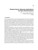
Fig. 12. Three allocation sets for five sink nodes in a nonuniform node-density wireless sensor
network obtained by the suppression particle swarm optimization algorithm.
Fig. 13. Average delivery ratio for a nonuniform node-density wireless sensor network. SPSO:
the suppression particle swarm optimization method. PSO: the particle swarm optimization
method. Regular: the regular allocation method.
5. Conclusions
This chapter has discussed a method of placing sink nodes effectively in an observation area
to use wireless sensor networks for a long time. For the effective search of sink node locations,
this chapter has presented the suppression particle swarm optimization method, which is a
new method based on the particle swarm optimization algorithm, to search several acceptable
solutions. In the actual environment of wireless sensor networks, natural conditions or other
factors may disturb the placement of a sink node at a selected location or the location effect
may be lost due to the appearance of a blocking object. Therefore, it is important to provide
several means (candidate locations) for sink nodes by using a method capable of searching
several acceptable solutions. In the simulation experiment, the effectiveness of the method
has been verified by comparison for the particle swarm optimization algorithm and the arti-
ficial immune system. Without increasing the number of search iterations, several solutions
(candidate locations) of approximately the same level as that by the existing particle swarm
optimization could be obtained. Future problems include evaluation for solving ability of the
Fig. 11. Fitness in each method for a nonuniform node-density wireless sensor network. SPSO:
the suppression particle swarm optimization. AIS: the artifical immune system. PSO: the
particle swarm optimization.
Algorithm SPSO AIS PSO
Best fitness 4800 5115 4800
Average fitness 4979 5429 4971
Number of solutions 3.51 6.17 1
Table 5. Fitness and the number of solutions for a nonuniform node-density wireless sen-
sor network. SPSO: the suppression particle swarm optimization. AIS: the artifical immune
system. PSO: the particle swarm optimization.

self-control mechanism and fitness does not converge monotonously. On the other hand, in
the particle swarm optimization algorithm, fitness converges to a single solution and it is not
possible to search other solutions. The number of obtained solutions in the artificial immune
system is the most, but fitness is the worst. The fitness in the suppression particle swarm op-
timization algorithm is almost the same as that in the particle swarm optimization algorithm.
Fig. 12 shows three allocation sets for five sink nodes finally obtained by the suppression par-
ticle swarm optimization algorithm. Fig. 13 shows average delivery ratio for three methods.
Sink node allocation sets obtained by all the methods are shown in Fig. 14.
As same as the previous experiment, the suppression particle swarm optimization algorithm
can keep higher average delivery ratio than the other methods. This means that for the
nonuniform node-density wireless sensor network, the suppression particle swarm optimiza-
tion algorithm can also search effective sink node allocation sets. Because, it is possible to
widely search on solution space. That is, the suppression particle swarm optimization method
is applicable to various wireless sensor networks, and can realize long-term operation of the
wireless sensor networks.
Sustainable Wireless Sensor Networks412
(a) (b) (c)
Fig. 14. Sink node allocation sets obtained by each method. (a) SPSO: the suppression particle
swarm optimization method. (b) PSO: the particle swarm optimization method. (c) Regular:
the regular allocation method.
method in more detail, and fusion with the existing communication algorithms dedicated to
wireless sensor networks.
6. References
Akyildiz, I.; Su, W.; Sankarasubramaniam, Y. & Cayirci, E. (2002). Wireless sensor networks:
A survey, Computer Networks Journal, Vol. 38, No. 4, 393-422
de Castro, L.; Timmis, J. (2002). Artificial immune systems: A new computational approach,
Springer, London.
Dubois-Ferriere, H.; Estrin, D. & Stathopoulos, T. (2004). Efficient and practical query scoping
in sensor networks, Proceedings of the IEEE International Conference on Mobile Ad-Hoc
and Sensor Systems, 564-566

Heinzelman, W.R.; Chandrakasan, A. & Balakrishnan, H. (2000). Energy-efficient communi-
cation protocol for wireless microsensor networks, Proceedings of Hawaii International
Conference on System Sciences, 3005–3014
Kennedy, J. & Eberhart, R.C. (1995). Particle swarm optimization, Proceedings of the IEEE Inter-
national Conference on Neural Networks, 1942-1948
Oyman, E.I. & Ersoy, C. (2004). Multiple sink network design problem in large scale wireless
sensor networks, Proceedings of the International Conference on Communications, Vol. 6,
3663-3667
Xia, L.; Chen, X. & Guan, X. (2004). A new gradient-based routing protocol in wireless sensor
networks, Lecture Notes in Computer Science, Vol. 3605, 318-325
Yoshimura, M.; Nakano, H.; Utani, A.; Miyauchi A. & Yamamoto, H. (2009). An Effective
Allocation Scheme for Sink Nodes in Wireless Sensor Networks Using Suppression
PSO, ICIC Express Letters, Vol. 3, No. 3(A), 519–524
Hybrid Approach for Energy-Aware Synchronization 413
Hybrid Approach for Energy-Aware Synchronization
Robert Akl, Yanos Saravanos and Mohamad Haidar
X

Hybrid Approach for
Energy-Aware Synchronization

Robert Akl, Yanos Saravanos and Mohamad Haidar
University of North Texas
Denton, Texas, USA

1. Introduction
Several sensor applications have been developed over the last few years to monitor
environmental properties such as temperature and humidity. One of the most important
requirements for these monitoring applications is being unobtrusive, which creates a need
for wireless ad-hoc networks using very small sensing nodes. These special networks are

called wireless sensor networks (WSN). WSNs are built from many wireless sensors in a
high-density configuration to provide redundancy and to monitor a large physical area.
WSNs can be used to detect traffic patterns within a city by tracking the number of vehicles
using a designated street (Winjie et al., 2005), (Tubaishat et al., 2008). If an emergency arises,
the network can relay the information to the city hall and notify police, fire, and ambulance
drivers of congested streets. An application could even be designed that suggests the fastest
route to the emergency area. When compared to computer terminals in Local Area
Networks (LANs), wireless sensors must operate on very low capacity batteries to minimize
their size to about that of a quarter. The nodes use slow processing units to conserve battery
power. A typical sensor node such as Crossbow’s Mica2DOT operates at 4 MHz with 4 KB
of memory and has a radio transceiver operating at up to 15 Kbps (MICA2DOT, 2005).
Radio transmissions consume by far the majority of the battery’s energy, so even with this
low-power hardware, a sensor can easily be depleted within a few hours if it is continuously
transmitting.
One of the most common uses for wireless sensor networks is for localization and
tracking(Patwari et al., 2005), (Langendoen & Reijers , 2003). Tracking of a single object is
relatively simple since data can be handed-off from sensor to sensor as the object moves
through the network.
Another important aspect is time synchronization in a networked system. The majority of
research in this field has concentrated on traditional high-speed computer networks with
few power restraints, leading to the Global Positioning System (GPS) and the Network Time
Protocol (NTP), (NTP, 2009). Although GPS is an accurate and commonly used
synchronization protocol, there are a few requirements that GPS fails to meet. Some of
which are that the receiver is 4.5 inches in diameter, more than 4 times the size of a typical
sensor node, and also requires an external power source. These two traits counteract the
goal of using small and mobile nodes to create a WSN, not to forget the line-of-sight
18
Sustainable Wireless Sensor Networks414

requirement that cripples GPS’s use for sensor networks dispersed within a building or in a

heavily forested area. On the other hand, NTP is one of the first synchronization protocols
used for computer systems, first developed in 1985 (NTP, 2009). This protocol uses a
relatively large amount of memory to store data for synchronization sources, authentication
codes, monitoring options, and access options. As mentioned earlier, typical wireless sensor
nodes have limited onboard memory. A large sensor network will require large files for
synchronization sources and codes. If these configuration files can be programmed into each
node, it would leave very little memory to hold the data monitored by the sensor, limiting
NTP’s use for WSNs. Furthermore, NTP’s synchronization accuracy is within 10 ms over the
Internet, and up to 200 μs in a LAN (NTP, 2009); these specifications are inadequate for most
sensor network applications. Therefore, new synchronization methods have been developed
specifically for sensor networks, such as the reference broadcast synchronization method
(RBS) (Elson et al., 2002) and the timing-sync protocol for sensor networks (TPSN)
(Ganeriwal, November 2003), (Ganeriwal, 2003).
RBS and TPSN achieve accurate clock synchronization within a few microseconds of
uncertainty nonetheless both are designed for networks with a small number of sensors and
are not specifically geared towards energy conservation. Although these algorithms tend to
work for larger networks, their energy consumption becomes inefficient and network
connectivity is broken once nodes begin lacking power. Simulations show that
synchronizing a large sensor network requires a large number of transmissions, which will
quickly deplete sensors and reduce the network’s coverage area.
A time synchronization scheme for wireless sensor networks that aims to save sensor
battery power while maintaining network connectivity for as long as possible is presented
based on a hybrid algortihm that combines both TPSN and RBS.
This algorithm is an extension of our previous work presented in (Akl & Saravanos, 2007). It
focuses on the following aspects of WSNs:
1. Design a hybrid method between RBS and TPSN to reduce the number of
transmissions required to synchronize an entire network.
2. Extend single-hop synchronization methods to operate in large multi-hop
networks.
3. Verify that the hybrid method operates as desired by simulating against RBS and

TPSN.
4. Maintain network connectivity and coverage.

2. Time Synchronization Algorithms in WSNs
Traditional synchronization methods, that are effective for computer networks, are
ineffective in sensor networks. New synchronization algorithms specifically designed for
wireless sensor networks have been developed and can be used for several applications
(Sivirkaya & Yener, 2004). The authors in (Palchaudhuri et al., 2004) present a probabilistic
method for clock synchronization based on RBS. In (Sun et al., 2006), the authors present a
level-based and a diffusion-based clock synchronization that is resilient to some source
nodes. The authors in (He & Kuo, 2006) propose creating spanning trees with multiple
subtrees in which two subtree synchronization algorithms can be performed. Four methods
are described in (Qun & Rus, 2006) to achieve global synchronization: a node-based, a
hierarchal cluster-based, a diffusion-based, and a fault-tolerant based approach. An Efficient

RBS (E-RBS) algorithm is proposed in (Lee et al., 2006) to decrease the number of messages
to be processed and save energy consumption within a given accuracy range.

2.1 The Reference Broadcast Synchronization Method (RBS)
Since GPS and NTP are not very effective in wireless sensor applications, the first major
research attempts to create a time synchronization algorithm specifically tailored for sensor
networks led to the development of reference broadcast synchronization (RBS) in 2002
(Elson et al., 2002). The algorithm defines a critical path, which is represented by the portion
of the network where a significant amount of clock uncertainty exists. A long critical path
results in high uncertainty and low accuracy in the synchronization. There are four main
sources of delays that must be accounted for to have accurate time synchronization:
 Send time: this is the time to create the message packet.
 Access time: this is a delay when the transmission medium is busy, forcing the
message to wait.
 Propagation time: this is the delay required for the message to traverse the

transmission medium from sender to receiver.
 Receive time: similar to the send time, this is the amount of time required for the
message to be processed once it is received.
The RBS algorithm can be split into three major events:
1. Flooding: a transmitter broadcasts a synchronization request packet.
2. Recording: the receivers record their local clock time when they initially pick up the
sync signal from the transmitter.
3. Exchange: the receivers exchange their observations with each other.

RBS synchronizes each set of receivers with each other as opposed to traditional algorithms
that synchronize receivers with senders. These latter algorithms have a long critical path,
starting from the initial send time until the receive time. For this reason, NTP’s accuracy is
severely limited, as discussed previously. RBS uses a relative time reference between nodes,
eliminating the send and access time uncertainties. The propagation delay of signals is
extremely fast from point-to-point, so this delay can be ignored when dealing in the
microsecond scale. Lastly, the receive time is reduced since RBS uses a relative difference in
times between receivers. Nonetheless, the time of reception is taken when the packet is first
received in the MAC layer, eliminating uncertainties introduced by the sensor’s processing
unit.
There are two unique implementations of RBS. The simplest method is designed for very
high accuracy for sparse networks, where transmitters have at most two receivers. The
transmitter can broadcast a synchronization request to the two receivers, which will record
the times at which they receive the request, just as the algorithm describes. However, the
receivers will exchange their observations with each other multiple times, using a linear
regression to lower the clock offset. The other version of the RBS algorithm involves the
following steps: the transmitter sends a reference packet to two receivers; each receiver
checks the time when it receives the reference packet; the receivers exchange their recorded
times. The main problems with this scheme are the nondeterministic behavior of the
receiver, as well as clock skew. The receiver’s nondeterministic behavior can be resolved by
simply sending more reference packets. The clock skew is resolved by using the slope of a

least-squares linear regression line to match the timing of the crystal oscillators.
Hybrid Approach for Energy-Aware Synchronization 415

requirement that cripples GPS’s use for sensor networks dispersed within a building or in a
heavily forested area. On the other hand, NTP is one of the first synchronization protocols
used for computer systems, first developed in 1985 (NTP, 2009). This protocol uses a
relatively large amount of memory to store data for synchronization sources, authentication
codes, monitoring options, and access options. As mentioned earlier, typical wireless sensor
nodes have limited onboard memory. A large sensor network will require large files for
synchronization sources and codes. If these configuration files can be programmed into each
node, it would leave very little memory to hold the data monitored by the sensor, limiting
NTP’s use for WSNs. Furthermore, NTP’s synchronization accuracy is within 10 ms over the
Internet, and up to 200 μs in a LAN (NTP, 2009); these specifications are inadequate for most
sensor network applications. Therefore, new synchronization methods have been developed
specifically for sensor networks, such as the reference broadcast synchronization method
(RBS) (Elson et al., 2002) and the timing-sync protocol for sensor networks (TPSN)
(Ganeriwal, November 2003), (Ganeriwal, 2003).
RBS and TPSN achieve accurate clock synchronization within a few microseconds of
uncertainty nonetheless both are designed for networks with a small number of sensors and
are not specifically geared towards energy conservation. Although these algorithms tend to
work for larger networks, their energy consumption becomes inefficient and network
connectivity is broken once nodes begin lacking power. Simulations show that
synchronizing a large sensor network requires a large number of transmissions, which will
quickly deplete sensors and reduce the network’s coverage area.
A time synchronization scheme for wireless sensor networks that aims to save sensor
battery power while maintaining network connectivity for as long as possible is presented
based on a hybrid algortihm that combines both TPSN and RBS.
This algorithm is an extension of our previous work presented in (Akl & Saravanos, 2007). It
focuses on the following aspects of WSNs:
1. Design a hybrid method between RBS and TPSN to reduce the number of

transmissions required to synchronize an entire network.
2. Extend single-hop synchronization methods to operate in large multi-hop
networks.
3. Verify that the hybrid method operates as desired by simulating against RBS and
TPSN.
4. Maintain network connectivity and coverage.

2. Time Synchronization Algorithms in WSNs
Traditional synchronization methods, that are effective for computer networks, are
ineffective in sensor networks. New synchronization algorithms specifically designed for
wireless sensor networks have been developed and can be used for several applications
(Sivirkaya & Yener, 2004). The authors in (Palchaudhuri et al., 2004) present a probabilistic
method for clock synchronization based on RBS. In (Sun et al., 2006), the authors present a
level-based and a diffusion-based clock synchronization that is resilient to some source
nodes. The authors in (He & Kuo, 2006) propose creating spanning trees with multiple
subtrees in which two subtree synchronization algorithms can be performed. Four methods
are described in (Qun & Rus, 2006) to achieve global synchronization: a node-based, a
hierarchal cluster-based, a diffusion-based, and a fault-tolerant based approach. An Efficient

RBS (E-RBS) algorithm is proposed in (Lee et al., 2006) to decrease the number of messages
to be processed and save energy consumption within a given accuracy range.

2.1 The Reference Broadcast Synchronization Method (RBS)
Since GPS and NTP are not very effective in wireless sensor applications, the first major
research attempts to create a time synchronization algorithm specifically tailored for sensor
networks led to the development of reference broadcast synchronization (RBS) in 2002
(Elson et al., 2002). The algorithm defines a critical path, which is represented by the portion
of the network where a significant amount of clock uncertainty exists. A long critical path
results in high uncertainty and low accuracy in the synchronization. There are four main
sources of delays that must be accounted for to have accurate time synchronization:

 Send time: this is the time to create the message packet.
 Access time: this is a delay when the transmission medium is busy, forcing the
message to wait.
 Propagation time: this is the delay required for the message to traverse the
transmission medium from sender to receiver.
 Receive time: similar to the send time, this is the amount of time required for the
message to be processed once it is received.
The RBS algorithm can be split into three major events:
1. Flooding: a transmitter broadcasts a synchronization request packet.
2. Recording: the receivers record their local clock time when they initially pick up the
sync signal from the transmitter.
3. Exchange: the receivers exchange their observations with each other.

RBS synchronizes each set of receivers with each other as opposed to traditional algorithms
that synchronize receivers with senders. These latter algorithms have a long critical path,
starting from the initial send time until the receive time. For this reason, NTP’s accuracy is
severely limited, as discussed previously. RBS uses a relative time reference between nodes,
eliminating the send and access time uncertainties. The propagation delay of signals is
extremely fast from point-to-point, so this delay can be ignored when dealing in the
microsecond scale. Lastly, the receive time is reduced since RBS uses a relative difference in
times between receivers. Nonetheless, the time of reception is taken when the packet is first
received in the MAC layer, eliminating uncertainties introduced by the sensor’s processing
unit.
There are two unique implementations of RBS. The simplest method is designed for very
high accuracy for sparse networks, where transmitters have at most two receivers. The
transmitter can broadcast a synchronization request to the two receivers, which will record
the times at which they receive the request, just as the algorithm describes. However, the
receivers will exchange their observations with each other multiple times, using a linear
regression to lower the clock offset. The other version of the RBS algorithm involves the
following steps: the transmitter sends a reference packet to two receivers; each receiver

checks the time when it receives the reference packet; the receivers exchange their recorded
times. The main problems with this scheme are the nondeterministic behavior of the
receiver, as well as clock skew. The receiver’s nondeterministic behavior can be resolved by
simply sending more reference packets. The clock skew is resolved by using the slope of a
least-squares linear regression line to match the timing of the crystal oscillators.
Sustainable Wireless Sensor Networks416

RBS can be adapted to work in multi-hop environments as well. Assuming a network has
grouped clusters with some overlapping receivers, linear regression can be used to
synchronize between receivers that are not immediate neighbors. However, it is more
complicated than the single-hop scenario since there will be timestamp conversions as the
packet is relayed through nodes. This extra complication is manifested in larger
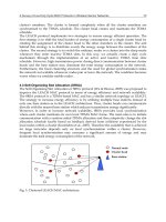
synchronization errors. Fig. 1 shows how a sensor network is synchronized by using RBS.


Fig. 1. RBS Synchronization of a Wireless Sensor Network (The initial solid dark lines
represent the network’s topology after flooding; the solid light lines represent transmitter-
to-receivers communication; the dashed lines represent receiver-to-receiver transmissions).

There are some issues with the RBS synchronization algorithm that must be addressed in an
energy-aware sensor network. First, the receiver-to-receiver synchronization method is
effective at reducing the critical path to increase the accuracy, but RBS scales poorly with
dense networks where there are many receivers for each transmitter. Given n receivers for a
single transmitter, the number of transmissions increases linearly with n, but the number of
receptions increases as O(n
2
). The following numbers of transmissions and receptions exist
in RBS:
RBS
TX n , (1)

2
1
1
( 1)
2 2
n
RBS
i
n n n n
RX n i n




    

(2)

For a large number of receivers per transmitter, this method becomes infeasible due to
energy constraints.
Lastly, RBS does not account for lost network coverage when nodes begin losing power.
Should a transmitting node be depleted, all of its receivers will be dropped from the
network, so measures should be taken to re-establish connectivity when the coverage
decreases beyond some threshold value.

2.2 TheTiming-Sync Protocol
The timing-sync protocol for sensor networks (TPSN) was developed in 2003 in an attempt
to further refine time synchronization beyond RBS’s capabilities (Ganeriwal, November
2003), (Ganeriwal, 2003). TPSN uses the same sources of uncertainty as RBS does (send,

access, propagation, and receive), with the addition of two more:
 Transmission time: the time for the packet to be processed and sent through the RF
transceiver during transmission.
 Access time: the time for each bit to be processed from the RF transceiver during
signal reception.

The TPSN works in two phases:
1. Level Discovery Phase: this is a very similar approach to the flooding phase in RBS,
where a hierarchical tree is created beginning from a root node.
2. Synchronization Phase: in this phase, pair-wise synchronization is performed
between each transmitter and receiver.
In the level discovery phase, each sensor node is assigned a level according to the
hierarchical tree. A pre-determined root node is assigned as level 0 and broadcasts a
level_discovery packet. Sensors that receive this packet are assigned as children to the
transmitter and are set as level 1 (they will ignore subsequent level_discovery packets). Each
of these nodes broadcasts a level_discovery packet, and the pattern continues with the level 2
nodes.
In the synchronization phase, pair-wise synchronization is performed between the
transmitter and receiver nodes using a 2-way handshake.
Although RBS removes the uncertainty at the sender by exchanging times amongst
receivers, TPSN reduces the remaining uncertainties by a factor of 2 due to the handshake
process that averages the clock drift and propagation delay. However, TPSN’s uncertainty
at the sender can be reduced to an insignificant delay by time-stamping at the MAC layer
just before the bits are sent through the transceiver.
The number of transmitters and receivers in TPSN are as follows:

1
TPSN
TX n


 , (3)
2
TPSN
R
X n

. (4)

Fig. 2 shows how a sensor network is synchronized by using TPSN.
Hybrid Approach for Energy-Aware Synchronization 417

RBS can be adapted to work in multi-hop environments as well. Assuming a network has
grouped clusters with some overlapping receivers, linear regression can be used to
synchronize between receivers that are not immediate neighbors. However, it is more
complicated than the single-hop scenario since there will be timestamp conversions as the
packet is relayed through nodes. This extra complication is manifested in larger
synchronization errors. Fig. 1 shows how a sensor network is synchronized by using RBS.


Fig. 1. RBS Synchronization of a Wireless Sensor Network (The initial solid dark lines
represent the network’s topology after flooding; the solid light lines represent transmitter-
to-receivers communication; the dashed lines represent receiver-to-receiver transmissions).

There are some issues with the RBS synchronization algorithm that must be addressed in an
energy-aware sensor network. First, the receiver-to-receiver synchronization method is
effective at reducing the critical path to increase the accuracy, but RBS scales poorly with
dense networks where there are many receivers for each transmitter. Given n receivers for a
single transmitter, the number of transmissions increases linearly with n, but the number of
receptions increases as O(n
2

). The following numbers of transmissions and receptions exist
in RBS:
RBS
TX n

, (1)

2
1
1
( 1)
2 2
n
RBS
i
n n n n
RX n i n


 
    

(2)

For a large number of receivers per transmitter, this method becomes infeasible due to
energy constraints.
Lastly, RBS does not account for lost network coverage when nodes begin losing power.
Should a transmitting node be depleted, all of its receivers will be dropped from the
network, so measures should be taken to re-establish connectivity when the coverage
decreases beyond some threshold value.

2.2 TheTiming-Sync Protocol
The timing-sync protocol for sensor networks (TPSN) was developed in 2003 in an attempt
to further refine time synchronization beyond RBS’s capabilities (Ganeriwal, November
2003), (Ganeriwal, 2003). TPSN uses the same sources of uncertainty as RBS does (send,
access, propagation, and receive), with the addition of two more:
 Transmission time: the time for the packet to be processed and sent through the RF
transceiver during transmission.
 Access time: the time for each bit to be processed from the RF transceiver during
signal reception.

The TPSN works in two phases:
1. Level Discovery Phase: this is a very similar approach to the flooding phase in RBS,
where a hierarchical tree is created beginning from a root node.
2. Synchronization Phase: in this phase, pair-wise synchronization is performed
between each transmitter and receiver.
In the level discovery phase, each sensor node is assigned a level according to the
hierarchical tree. A pre-determined root node is assigned as level 0 and broadcasts a
level_discovery packet. Sensors that receive this packet are assigned as children to the
transmitter and are set as level 1 (they will ignore subsequent level_discovery packets). Each
of these nodes broadcasts a level_discovery packet, and the pattern continues with the level 2
nodes.
In the synchronization phase, pair-wise synchronization is performed between the
transmitter and receiver nodes using a 2-way handshake.
Although RBS removes the uncertainty at the sender by exchanging times amongst
receivers, TPSN reduces the remaining uncertainties by a factor of 2 due to the handshake
process that averages the clock drift and propagation delay. However, TPSN’s uncertainty
at the sender can be reduced to an insignificant delay by time-stamping at the MAC layer
just before the bits are sent through the transceiver.
The number of transmitters and receivers in TPSN are as follows:

1
TPSN
TX n  , (3)
2
TPSN
R
X n . (4)

Fig. 2 shows how a sensor network is synchronized by using TPSN.
Sustainable Wireless Sensor Networks418


Fig. 2. TPSN Synchronization of a Wireless Sensor Network (The initial solid dark lines
represent the network’s topology after flooding; the subsequent light lines represent
successful transmitter-to-receiver synchronizations).

TPSN is a great improvement over RBS in terms of accuracy since it employs a 2-way
handshake, which reduces uncertainty to half since the average of the time differences is
used. However, the main drawback TPSN faces is that it consumes energy in sparse
networks; a 2-way handshake requires each node to receive a packet and to send one in
response. In addition, TPSN shares the same problem with RBS with respect to lost network
coverage when nodes begin losing power. A dead transmitter node will drop all of its
receivers from the network, lowering the WSN’s coverage area. Network restructuring is
not included in the TPSN algorithm.
RBS and TPSN are some of the first efforts in creating synchronization algorithms tailored
towards low-power sensor networks. They both have unique strengths when dealing with
energy consumption. RBS is most effective in networks where transmitting sensors have few
receivers, while TPSN excels when transmitters have many receivers.

2.3 Energy-Aware Time Sychronization
A new hybrid algorithm is proposed in this section.

2.3.1 Hybrid Flooding
Before the sensors can be synchronized, a network topology must be created. Table 1 shows
the algorithm for the hybrid flooding algorithm that is used by each sensor node to
efficiently flood the network.

Algorithm 1: Hybrid Flooding Algorithm
Accept flood_packets
Set receiver_threshold to low_power
Set num_receivers to 0
If current_node is root node
Broadcast flood_packet
Else If current_node receives flood_packet and is accepting them
Set parent of current_node to source of broadcast
Set current_node level to parent’s node level + 1
Rebroadcast flood request with current_node ID and level
Broadcast ack_packet with current_node ID
Ignore subsequent flood_packets
Else If current_node receives ack_packet
Increment num_receivers
Table 1. The Hybrid Flooding algorithm

Each sensor is initially set to accept flood_packets, but will ignore subsequent ones in order
not to be continuously reassigned as the flood broadcast propagates. The num_receivers

variable keeps track of the node’s receivers and is used in the synchronization algorithm.

2.3.2 Hybrid Synchronization
Once the network flooding has been completed, the network can be synchronized using the
determined hierarchy. In networks where the sensors are dispersed at random, there will be
patches of high density node distribution interspersed with lower density regions. A
transmitter in a high density area will usually have a large number of receivers, while
another transmitter in a lower density section will usually have 1 or 2 receivers at most. As
discussed in the previous sections, RBS excels when the transmitter has few receivers and
TPSN excels with many receivers connected to each transmitter.
The hybrid algorithm minimizes power regardless of the network’s topology by choosing
the best synchronization technique depending on the number of children connected to the
transmitter. Since the energy required for reception usually differs from that of a
transmission, the ratio of the reception power to the transmission power is needed in order
to find the optimal point at which to switch from receiver-receiver synchronization to
transmitter-receiver synchronization. In order to find the ratio of reception-to-transmission
power, α, we combine equations (1), (2), (3), and (4):
Hybrid Approach for Energy-Aware Synchronization 419


Fig. 2. TPSN Synchronization of a Wireless Sensor Network (The initial solid dark lines
represent the network’s topology after flooding; the subsequent light lines represent
successful transmitter-to-receiver synchronizations).

TPSN is a great improvement over RBS in terms of accuracy since it employs a 2-way
handshake, which reduces uncertainty to half since the average of the time differences is
used. However, the main drawback TPSN faces is that it consumes energy in sparse
networks; a 2-way handshake requires each node to receive a packet and to send one in
response. In addition, TPSN shares the same problem with RBS with respect to lost network
coverage when nodes begin losing power. A dead transmitter node will drop all of its

receivers from the network, lowering the WSN’s coverage area. Network restructuring is
not included in the TPSN algorithm.
RBS and TPSN are some of the first efforts in creating synchronization algorithms tailored
towards low-power sensor networks. They both have unique strengths when dealing with
energy consumption. RBS is most effective in networks where transmitting sensors have few
receivers, while TPSN excels when transmitters have many receivers.





2.3 Energy-Aware Time Sychronization
A new hybrid algorithm is proposed in this section.

2.3.1 Hybrid Flooding
Before the sensors can be synchronized, a network topology must be created. Table 1 shows
the algorithm for the hybrid flooding algorithm that is used by each sensor node to
efficiently flood the network.

Algorithm 1: Hybrid Flooding Algorithm
Accept flood_packets
Set receiver_threshold to low_power
Set num_receivers to 0
If current_node is root node
Broadcast flood_packet
Else If current_node receives flood_packet and is accepting them
Set parent of current_node to source of broadcast
Set current_node level to parent’s node level + 1
Rebroadcast flood request with current_node ID and level
Broadcast ack_packet with current_node ID

Ignore subsequent flood_packets
Else If current_node receives ack_packet
Increment num_receivers
Table 1. The Hybrid Flooding algorithm

Each sensor is initially set to accept flood_packets, but will ignore subsequent ones in order
not to be continuously reassigned as the flood broadcast propagates. The num_receivers
variable keeps track of the node’s receivers and is used in the synchronization algorithm.

2.3.2 Hybrid Synchronization
Once the network flooding has been completed, the network can be synchronized using the
determined hierarchy. In networks where the sensors are dispersed at random, there will be
patches of high density node distribution interspersed with lower density regions. A
transmitter in a high density area will usually have a large number of receivers, while
another transmitter in a lower density section will usually have 1 or 2 receivers at most. As
discussed in the previous sections, RBS excels when the transmitter has few receivers and
TPSN excels with many receivers connected to each transmitter.
The hybrid algorithm minimizes power regardless of the network’s topology by choosing
the best synchronization technique depending on the number of children connected to the
transmitter. Since the energy required for reception usually differs from that of a
transmission, the ratio of the reception power to the transmission power is needed in order
to find the optimal point at which to switch from receiver-receiver synchronization to
transmitter-receiver synchronization. In order to find the ratio of reception-to-transmission
power, α, we combine equations (1), (2), (3), and (4):
Sustainable Wireless Sensor Networks420

2
2
( 3 )
TPSN RBS

RBS TPSN
TX TX
n
R
X RX n n


 
  
(5)

In general, the following equation can be used to determine the receiver_threshold by solving
equation (5) for n:
2
2
3 0n n

   (6)

Table 2 shows the algorithm for the hybrid Synchronization algorithm.

Algorithm 2: Hybrid Synchronization Algorithm
Set receiver_threshold to high_power
If num_receivers < receiver_threshold // Use RBS algorithm
Transmitter broadcasts sync_request
For each receiver
Record local time of reception for sync_request
Broadcast observation_packet
Receive observation_packet from other receivers
Else // Use TPSN algorithm

Transmitter broadcasts sync_request
For each receiver
Record local time of reception for sync_request
Broadcast ack_packet to transmitter with local time
Table 2. The Hybrid Synchronization Algorithm

2.3.3 Energy Depletion
Another issue that the hybrid algorithm addresses when synchronizing a sensor network is
the effect that a depleted sensor has on the topology. Once the battery is exhausted, the node
will be dropped from the network, but so will all of the receivers depending on it. This loss
of connectivity cascades through each receiver, so a drastic restructuring can occur when a
high-level sensor is drained. The hybrid algorithm keeps track of the number of powered
nodes. Once this number decreases below another user-defined threshold, the network is
re-flooded using the flooding algorithm described earlier in Table 2. Should the source node
lose power, a new source node is chosen from the original one’s receivers. These receivers
communicate their power levels with each other and the one with the most remaining
energy is elected as the new root node, as show in Table 3.







Algorithm 3: Root Node Election Algorithm
If cur_node_level == 1 and cur_node_power allows 1 more TX
Broadcast elect_packet with cur_node_ID
If cur_node_level == 2
Broadcast elect_packet with cur_node_ID, cur_node_power
If cur_node receives elect_packet and elect_packet_power >= cur_node_power

Set elect_packet_ID to root node

Table 3.
The Root Node Election Algorithm

In addition, receivers will only analyze the sync_request packets from their respective
transmitters when using the TPSN-style synchronization. This saves additional battery
power since the receivers do not have to analyze packets they overhear from other
broadcasting transmitters. Lastly, the dropped packets are monitored. This is a useful
statistic since it keeps track of algorithm efficiency and wasted energy. Dropped packets also
allow us to compare various network topologies and determine which ones allow for the
most energy conservation.

3. Results and Analysis

3.1 Hybrid Algorithm Validation
Several simulations were run to compare the power consumption of the TPSN, the RBS, and
our hybrid algorithm discussed in the previous section. A transmitting sensor can
dynamically switch between RBS and TPSN by simply comparing the number of connected
receivers to the reception/transmission power ratio. This ratio is changed in order to
observe how each of the algorithms is affected. All other parameters are kept constant. Our
simulations are run on a 1000m x 1000m area, which is randomly populated with 500
sensors, and the path loss coefficient is set to 3.5. In each simulation, the receiver_threshold
value is changed from 1 to the largest number of receivers connected to a sensor. The
hybrid synchronization algorithm is executed for each of these receiver_threshold values and
the energy consumption is stored and compared to the consumption of TPSN, RBS, and the
optimal hybrid synchronization algorithm. Each of the data points is plotted, along with a
line representing the average from all of the simulations. For the MICA2Dot platform, a
reception uses approximately 24 mW of power, while a transmission requires 75 mW at -5
dBm (MICA2DOT, 2005). Solving for α and n in equations (5) and (6), we get α= 0.32 and n=

4.42, respectively.
The hybrid algorithm will use the least amount of energy when the receiver_threshold is set to
4.42. This means that transmitters with 4 or fewer sensors will use RBS for synchronization
while those with 5 or more receivers will use TPSN. Fig. 3 illustrates how changes in the
receiver_threshold value affect the hybrid algorithm.

Hybrid Approach for Energy-Aware Synchronization 421

2
2
( 3 )
TPSN RBS
RBS TPSN
TX TX
n
R
X RX n n


 
  
(5)

In general, the following equation can be used to determine the receiver_threshold by solving
equation (5) for n:
2
2
3 0n n



  (6)

Table 2 shows the algorithm for the hybrid Synchronization algorithm.

Algorithm 2: Hybrid Synchronization Algorithm
Set receiver_threshold to high_power
If num_receivers < receiver_threshold // Use RBS algorithm
Transmitter broadcasts sync_request
For each receiver
Record local time of reception for sync_request
Broadcast observation_packet
Receive observation_packet from other receivers
Else // Use TPSN algorithm
Transmitter broadcasts sync_request
For each receiver
Record local time of reception for sync_request
Broadcast ack_packet to transmitter with local time
Table 2. The Hybrid Synchronization Algorithm

2.3.3 Energy Depletion
Another issue that the hybrid algorithm addresses when synchronizing a sensor network is
the effect that a depleted sensor has on the topology. Once the battery is exhausted, the node
will be dropped from the network, but so will all of the receivers depending on it. This loss
of connectivity cascades through each receiver, so a drastic restructuring can occur when a
high-level sensor is drained. The hybrid algorithm keeps track of the number of powered
nodes. Once this number decreases below another user-defined threshold, the network is
re-flooded using the flooding algorithm described earlier in Table 2. Should the source node
lose power, a new source node is chosen from the original one’s receivers. These receivers
communicate their power levels with each other and the one with the most remaining
energy is elected as the new root node, as show in Table 3.

Algorithm 3: Root Node Election Algorithm
If cur_node_level == 1 and cur_node_power allows 1 more TX
Broadcast elect_packet with cur_node_ID
If cur_node_level == 2
Broadcast elect_packet with cur_node_ID, cur_node_power
If cur_node receives elect_packet and elect_packet_power >= cur_node_power
Set elect_packet_ID to root node

Table 3. The Root Node Election Algorithm

In addition, receivers will only analyze the sync_request packets from their respective
transmitters when using the TPSN-style synchronization. This saves additional battery
power since the receivers do not have to analyze packets they overhear from other
broadcasting transmitters. Lastly, the dropped packets are monitored. This is a useful
statistic since it keeps track of algorithm efficiency and wasted energy. Dropped packets also
allow us to compare various network topologies and determine which ones allow for the
most energy conservation.

3. Results and Analysis

3.1 Hybrid Algorithm Validation
Several simulations were run to compare the power consumption of the TPSN, the RBS, and
our hybrid algorithm discussed in the previous section. A transmitting sensor can

dynamically switch between RBS and TPSN by simply comparing the number of connected
receivers to the reception/transmission power ratio. This ratio is changed in order to
observe how each of the algorithms is affected. All other parameters are kept constant. Our
simulations are run on a 1000m x 1000m area, which is randomly populated with 500
sensors, and the path loss coefficient is set to 3.5. In each simulation, the receiver_threshold
value is changed from 1 to the largest number of receivers connected to a sensor. The
hybrid synchronization algorithm is executed for each of these receiver_threshold values and
the energy consumption is stored and compared to the consumption of TPSN, RBS, and the
optimal hybrid synchronization algorithm. Each of the data points is plotted, along with a
line representing the average from all of the simulations. For the MICA2Dot platform, a
reception uses approximately 24 mW of power, while a transmission requires 75 mW at -5
dBm (MICA2DOT, 2005). Solving for α and n in equations (5) and (6), we get α= 0.32 and n=
4.42, respectively.
The hybrid algorithm will use the least amount of energy when the receiver_threshold is set to
4.42. This means that transmitters with 4 or fewer sensors will use RBS for synchronization
while those with 5 or more receivers will use TPSN. Fig. 3 illustrates how changes in the
receiver_threshold value affect the hybrid algorithm.

Sustainable Wireless Sensor Networks422


Fig. 3. Mica2DOT Synchronization Comparison

The energy consumption from the hybrid algorithm when using the optimal
receiver_threshold value is lower than both TPSN and RBS. The minimum value is found
between values of 4 and 5. Lastly, the spread amongst data points increases dramatically as
the receiver threshold increases beyond 13.
More importantly, setting the receiver_threshold value to 1 will force a transmitter to use
TPSN. The hybrid algorithm in this case will have the same energy consumption as TPSN.
On the other hand, a receiver_threshold set to the largest number of receivers connected to a

transmitter will force a transmitter to use RBS.
The hybrid synchronization algorithm is very dynamic and will adapt itself to multiple
equipment specifications. The power requirements for the MicaZ sensor platform are
drastically different from the Mica2DOT platform; MicaZ uses 59.1 mW for a reception, but
only uses 42 mW for each transmission at -5 dBm (MICAz, 2005). Similarly, solving for α and
n in equations (5) and (6), we get α= 1.407 and n= 3.42, respectively. When using MicaZ, the
optimal receiver_threshold value is 3.42. This property is reflected in Fig. 4.,where the local
minimum has shifted further to the left when compared to the Mica2DOT platform.


Fig. 4. MicaZ Synchronization Comparison


Fig. 5. Synchronization Comparison for Architecture with n=6
Hybrid Approach for Energy-Aware Synchronization 423


Fig. 3. Mica2DOT Synchronization Comparison

The energy consumption from the hybrid algorithm when using the optimal
receiver_threshold value is lower than both TPSN and RBS. The minimum value is found
between values of 4 and 5. Lastly, the spread amongst data points increases dramatically as
the receiver threshold increases beyond 13.
More importantly, setting the receiver_threshold value to 1 will force a transmitter to use
TPSN. The hybrid algorithm in this case will have the same energy consumption as TPSN.
On the other hand, a receiver_threshold set to the largest number of receivers connected to a
transmitter will force a transmitter to use RBS.
The hybrid synchronization algorithm is very dynamic and will adapt itself to multiple
equipment specifications. The power requirements for the MicaZ sensor platform are
drastically different from the Mica2DOT platform; MicaZ uses 59.1 mW for a reception, but

only uses 42 mW for each transmission at -5 dBm (MICAz, 2005). Similarly, solving for α and
n in equations (5) and (6), we get α= 1.407 and n= 3.42, respectively. When using MicaZ, the
optimal receiver_threshold value is 3.42. This property is reflected in Fig. 4.,where the local
minimum has shifted further to the left when compared to the Mica2DOT platform.


Fig. 4. MicaZ Synchronization Comparison


Fig. 5. Synchronization Comparison for Architecture with n=6
Sustainable Wireless Sensor Networks424

Despite the differences in architecture, both of the above examples yield relatively similar
values for the optimal receiver_threshold. Assume that there is an improvement in the
Mica2DOT platform which allows for much lower power in receiving mode. Each
transmission still requires 75 mW at -5 dBm, but only 8 mW is needed for a reception. Then,
α and n from equations (5) and (6) are 0.107 and 6, respectively. Fig. 5 illustrates the energy
usage when the receiver_threshold changes.

In this particular example, the hybrid algorithm produces a local minimum when using the
optimal receiver_threshold, as was expected. It is also interesting to note that now, RBS
becomes more energy efficient than TPSN.

3.2 Power Consumption
The next set of simulations demonstrates the algorithm’s reduction in power consumption in
several network sizes. The number of sensors was changed from 250 up to 1500, in increments of
250. Just as before, 20 simulations were run over a 1000m x 1000m area which was randomly
populated with 500 sensors, and the path loss coefficient was set to 3.5. The Mica2DOT platform
was used and the ratio of reception/transmission power remained fixed. The receiver_threshold
value is once again changed from 1 to the largest number of receivers connected to a sensor. The

hybrid synchronization algorithm is executed for each of these receiver_threshold values and the
energy consumption is stored and compared to the consumption of TPSN, RBS, and the optimal
hybrid synchronization algorithm. Each of the data points is plotted, along with a line
representing the average from all of the simulations as show in Fig. 6, Fig. 7, and Fig. 8.


Fig. 6. Energy usage consumption for 500 sensors between RBS, TPSN, and our Hybrid algorithm
for different values of receiver_threshold values using Mica2Dot platform. Energy usage is in mW.


Fig. 7.Energy usage consumption for 1000 sensors between RBS, TPSN, and our Hybrid
algorithm for different values of receiver_threshold values using Mica2Dot platform. Energy
usage is in mW.


Fig. 8. Energy usage consumption for 1500 sensors between RBS, TPSN, and our Hybrid
algorithm for different values of receiver_threshold values using Mica2Dot platform. Energy
usage is in mW.
Hybrid Approach for Energy-Aware Synchronization 425

Despite the differences in architecture, both of the above examples yield relatively similar
values for the optimal receiver_threshold. Assume that there is an improvement in the
Mica2DOT platform which allows for much lower power in receiving mode. Each
transmission still requires 75 mW at -5 dBm, but only 8 mW is needed for a reception. Then,
α and n from equations (5) and (6) are 0.107 and 6, respectively. Fig. 5 illustrates the energy
usage when the receiver_threshold changes.

In this particular example, the hybrid algorithm produces a local minimum when using the
optimal receiver_threshold, as was expected. It is also interesting to note that now, RBS
becomes more energy efficient than TPSN.

3.2 Power Consumption
The next set of simulations demonstrates the algorithm’s reduction in power consumption in
several network sizes. The number of sensors was changed from 250 up to 1500, in increments of
250. Just as before, 20 simulations were run over a 1000m x 1000m area which was randomly
populated with 500 sensors, and the path loss coefficient was set to 3.5. The Mica2DOT platform
was used and the ratio of reception/transmission power remained fixed. The receiver_threshold
value is once again changed from 1 to the largest number of receivers connected to a sensor. The
hybrid synchronization algorithm is executed for each of these receiver_threshold values and the
energy consumption is stored and compared to the consumption of TPSN, RBS, and the optimal
hybrid synchronization algorithm. Each of the data points is plotted, along with a line
representing the average from all of the simulations as show in Fig. 6, Fig. 7, and Fig. 8.


Fig. 6. Energy usage consumption for 500 sensors between RBS, TPSN, and our Hybrid algorithm
for different values of receiver_threshold values using Mica2Dot platform. Energy usage is in mW.


Fig. 7.Energy usage consumption for 1000 sensors between RBS, TPSN, and our Hybrid
algorithm for different values of receiver_threshold values using Mica2Dot platform. Energy
usage is in mW.


Fig. 8. Energy usage consumption for 1500 sensors between RBS, TPSN, and our Hybrid
algorithm for different values of receiver_threshold values using Mica2Dot platform. Energy
usage is in mW.
Sustainable Wireless Sensor Networks426

As more sensors are introduced into the network, RBS becomes dramatically less feasible for
a wireless sensor network. As shown in Table 4, the hybrid algorithm’s energy savings over

RBS increases from 58% with 750 sensors to over 74% when the network uses 1500 sensors.

Sensors 250 500 750 1000 1250 1500
RBS
615 1709 3421 5510 7833 11128
TPSN
498 998 1498 1998 2498 2998
Hybrid
447 924 1415 1898 2386 2879
RBS Savings
27.44 % 45.94 % 58.65 % 65.55 % 69.54 % 74.13 %
TPSN
Savings
10.27 % 7.43 % 5.57 % 4.99 % 4.47 % 3.97 %
Table 4. Average Number of Receptions

In contrast, as the network becomes large, the hybrid algorithm mimics TPSN’s behavior,
but uses less energy. The difference is 5.57% with 750 sensors and 3.97% with 1500 sensors.
Although the number of receptions when using TPSN increases linearly with network size,
this number increases much more quickly when using RBS. The hybrid algorithm greatly
reduces the number of receptions when compared to RBS; for small networks, the advantage
is 27%, but it increases to over 74% in networks with a large number of sensors. Therefore,
the hybrid algorithm has a large advantage over TPSN in small networks, but that
advantage decreases as more sensors are added.
Table 5 shows the standard deviation in the number of receptions for each of the
synchronization algorithms. These results help to determine how sensitive an algorithm is to
modifications in the network’s topology and sensor density.

Sensors 250 500 750 1000 1250 1500
RBS

54.71
8.89 %
150.09
8.78 %
365.43
10.68 %
524.32
9.52 %
614.26
7.84 %
1129.50
10.15 %
TPSN
0.73
0.15 %
0.00
0.00 %
0.00
0.00 %
0.00
0.00 %
0.00
0.00 %
0.00
0.00 %
Hybrid
11.73
2.63 %
13.16
1.42 %

15.89
1.12 %
14.75
0.78 %
15.99
0.67 %
16.77
0.58 %
Table 5. Standard Deviation for Receptions

The table above shows that there is very large variation in the number of receptions for RBS,
meaning that the number of receptions when using RBS is highly dependent on the
topology of the network. The table also shows that the deviation in receptions when using
TPSN is usually 0, with the exception once again in the 250 sensor network. This exception is
due to orphaned nodes which do not participate in the synchronization. The hybrid
algorithm has a relatively low deviation, which decreases further with large numbers of
sensors. This behavior is attributed to the hybrid algorithm behaving similarly to TPSN
when the network is large.

Another simulation results are shown in Table 6 and Table 7. These results show that RBS’s
energy consumption is more dependent on the density of sensors in a given area. In
contrast, TPSN and the hybrid algorithm are less affected by the size of the network.

Sensors 250 500 750 1000 1250 1500
RBS
446 1046 1844 2762 3756 5060
TPSN
511 983 1434 1885 2331 2770
Hybrid
404 828 1253 1672 2095 2514

RBS Savings
9.29% 20.79% 32.04% 39.46% 44.22% 50.31%
TPSN
Savings
20.80% 15.73% 12.65% 11.28% 10.11% 9.23%
Table 6. Average Energy Consumption in mW

Sensors 250 500 750 1000 1250 1500
RBS
17.38
3.90%
48.03
4.59%
116.94
6.34%
167.78
6.07%
196.56
5.23%
361.44
7.14%
TPSN
7.67
1.50%
8.88
0.90%
14.31
1.00%
14.48
0.77%

18.22
0.78%
22.09
0.80%
Hybrid
4.00
0.99%
4.72
0.57%
5.23
0.42%
6.85
0.41%
6.33
0.30%
6.84
0.27%
Table 7.
Standard Deviation of Energy Consumption

When the network size increases from 250 sensors to 500 sensors (for the same area of 1
km
2
), RBS becomes less energy efficient than TPSN. The hybrid algorithm outperforms
TPSN by 15.7%, while outperforming RBS by 20.8%. Once the network increases to 750
sensors, RBS clearly becomes less efficient than TPSN. The hybrid algorithm still
outperforms TPSN by 12.7%. Since RBS consumes more energy, the hybrid algorithm now
outperforms it by 32%. As more sensors are introduced into the network, RBS becomes
dramatically less feasible for a wireless sensor network. As shown in Table I, the hybrid
algorithm’s energy savings over RBS increases from 39% with 1000 sensors to over 50%

when the network uses 1500 sensors. In contrast, as the network becomes large, the hybrid
algorithm mimics TPSN’s behavior, but uses less energy. The energy savings over TPSN are
11% with 1000 sensors and 9% with 1500 sensors. For extremely large networks (10,000+
sensors) TPSN has the same efficiency as our proposed algorithm.

4. Conclusion and Future Work
Wireless sensor networks have tremendous advantages for monitoring object movement
and environmental properties but require some degree of synchronization to achieve the
best results. The hybrid synchronization algorithm was designed to switch between Timing-
sync Protocol for Sensor Networks (TPSN) and the Reference Broadcast Synchronization
algorithm (RBS). These two algorithms allow all the sensors in a network to synchronize
themselves within a few microseconds of each other, while at the same time using the least
amount of energy possible. The savings in energy varies upon the density of the sensors as
Hybrid Approach for Energy-Aware Synchronization 427

As more sensors are introduced into the network, RBS becomes dramatically less feasible for
a wireless sensor network. As shown in Table 4, the hybrid algorithm’s energy savings over
RBS increases from 58% with 750 sensors to over 74% when the network uses 1500 sensors.

Sensors 250 500 750 1000 1250 1500
RBS
615 1709 3421 5510 7833 11128
TPSN
498 998 1498 1998 2498 2998
Hybrid
447 924 1415 1898 2386 2879
RBS Savings
27.44 % 45.94 % 58.65 % 65.55 % 69.54 % 74.13 %
TPSN
Savings

10.27 % 7.43 % 5.57 % 4.99 % 4.47 % 3.97 %
Table 4. Average Number of Receptions

In contrast, as the network becomes large, the hybrid algorithm mimics TPSN’s behavior,
but uses less energy. The difference is 5.57% with 750 sensors and 3.97% with 1500 sensors.
Although the number of receptions when using TPSN increases linearly with network size,
this number increases much more quickly when using RBS. The hybrid algorithm greatly
reduces the number of receptions when compared to RBS; for small networks, the advantage
is 27%, but it increases to over 74% in networks with a large number of sensors. Therefore,
the hybrid algorithm has a large advantage over TPSN in small networks, but that
advantage decreases as more sensors are added.
Table 5 shows the standard deviation in the number of receptions for each of the
synchronization algorithms. These results help to determine how sensitive an algorithm is to
modifications in the network’s topology and sensor density.

Sensors 250 500 750 1000 1250 1500
RBS
54.71
8.89 %
150.09
8.78 %
365.43
10.68 %
524.32
9.52 %
614.26
7.84 %
1129.50
10.15 %
TPSN

0.73
0.15 %
0.00
0.00 %
0.00
0.00 %
0.00
0.00 %
0.00
0.00 %
0.00
0.00 %
Hybrid
11.73
2.63 %
13.16
1.42 %
15.89
1.12 %
14.75
0.78 %
15.99
0.67 %
16.77
0.58 %
Table 5. Standard Deviation for Receptions

The table above shows that there is very large variation in the number of receptions for RBS,
meaning that the number of receptions when using RBS is highly dependent on the
topology of the network. The table also shows that the deviation in receptions when using

TPSN is usually 0, with the exception once again in the 250 sensor network. This exception is
due to orphaned nodes which do not participate in the synchronization. The hybrid
algorithm has a relatively low deviation, which decreases further with large numbers of
sensors. This behavior is attributed to the hybrid algorithm behaving similarly to TPSN
when the network is large.

Another simulation results are shown in Table 6 and Table 7. These results show that RBS’s
energy consumption is more dependent on the density of sensors in a given area. In
contrast, TPSN and the hybrid algorithm are less affected by the size of the network.

Sensors 250 500 750 1000 1250 1500
RBS
446 1046 1844 2762 3756 5060
TPSN
511 983 1434 1885 2331 2770
Hybrid
404 828 1253 1672 2095 2514
RBS Savings
9.29% 20.79% 32.04% 39.46% 44.22% 50.31%
TPSN
Savings
20.80% 15.73% 12.65% 11.28% 10.11% 9.23%
Table 6. Average Energy Consumption in mW

Sensors 250 500 750 1000 1250 1500
RBS
17.38
3.90%
48.03
4.59%

116.94
6.34%
167.78
6.07%
196.56
5.23%
361.44
7.14%
TPSN
7.67
1.50%
8.88
0.90%
14.31
1.00%
14.48
0.77%
18.22
0.78%
22.09
0.80%
Hybrid
4.00
0.99%
4.72
0.57%
5.23
0.42%
6.85
0.41%

6.33
0.30%
6.84
0.27%
Table 7. Standard Deviation of Energy Consumption

When the network size increases from 250 sensors to 500 sensors (for the same area of 1
km
2
), RBS becomes less energy efficient than TPSN. The hybrid algorithm outperforms
TPSN by 15.7%, while outperforming RBS by 20.8%. Once the network increases to 750
sensors, RBS clearly becomes less efficient than TPSN. The hybrid algorithm still
outperforms TPSN by 12.7%. Since RBS consumes more energy, the hybrid algorithm now
outperforms it by 32%. As more sensors are introduced into the network, RBS becomes
dramatically less feasible for a wireless sensor network. As shown in Table I, the hybrid
algorithm’s energy savings over RBS increases from 39% with 1000 sensors to over 50%
when the network uses 1500 sensors. In contrast, as the network becomes large, the hybrid
algorithm mimics TPSN’s behavior, but uses less energy. The energy savings over TPSN are
11% with 1000 sensors and 9% with 1500 sensors. For extremely large networks (10,000+
sensors) TPSN has the same efficiency as our proposed algorithm.

4. Conclusion and Future Work
Wireless sensor networks have tremendous advantages for monitoring object movement
and environmental properties but require some degree of synchronization to achieve the
best results. The hybrid synchronization algorithm was designed to switch between Timing-
sync Protocol for Sensor Networks (TPSN) and the Reference Broadcast Synchronization
algorithm (RBS). These two algorithms allow all the sensors in a network to synchronize
themselves within a few microseconds of each other, while at the same time using the least
amount of energy possible. The savings in energy varies upon the density of the sensors as
Sustainable Wireless Sensor Networks428

well as the reception-to-transmission ratio of energy usage; networks, which are saturated
with sensors, for example 1500 sensors in a 1 km
2
area, will favor TPSN over RBS. TPSN also
becomes more favorable as receptions consume more power. The hybrid algorithm
compromises between both of these previous algorithms. The energy savings over RBS can
range from 9.3% in small networks of 250 sensors, to over 50% for large networks using 1500
sensors. In contrast, the hybrid algorithm’s savings over TPSN range from 20.8% in the same
small networks down to 9% in the large networks. Furthermore, analysis of the standard
deviation for each of the algorithms shows RBS’s energy consumption can vary
dramatically, from nearly 4% to over 7%, generally increasing for larger networks. In
contrast, the standard deviation for TPSN’s energy usage decreases from 1.5% to less than
1%, generally decreasing for larger networks. The hybrid algorithm’s deviation is always
less than 1% and continuously decreases to 0.3% as more sensors are used.

5. References
Akl, R. & Saravanos, S. Hybrid Energy-Aware Synchronization Algorithm in Wireless
Sensor Networks, 18
th
IEEE International Symposium on Personal, Indoor, and Mobile
Radio Communications, PIMRC’07, pp. 1-5, September 2007, Athens.
Crossbow MICAz Wireless Measurement System, Document Part Number 6020-0060-03 Rev A,

MICAz_Datasheet.pdf
Elson, J.; Girod, L. & Estrin, D. Fine-Grained Network Time Synchronization using
Reference Broadcasts, Proceedings of the Fifth Symposium on Operating Systems Design
and Implementation (OSDI 2002), December 2002, Boston.
Ganeriwal, S.; Kumar, R. & Srivastava, M. Timing Sync Protocol for Sensor Networks, ACM
SenSys ’03, pp. 138-149, November 2003, Los Angeles.

Ganeriwal, S. & Srivastava, M. Timing-sync Protocol for Sensor Networks (TPSN) on
Berkeley Motes, NESL, 2003.
He, L. & Kuo, G. A Novel Time Synchronization Scheme in Wireless Sensor Networks, IEEE
63
rd
Vehicular Technology Conference, VTC 200,. pp. 568-572, May 2006, Melbourne.
Langendoen, K. & Reijers, N. (2003). Distributed Localization in Wireless Sensor Networks:
A Quantitative Comparison. The International Journal of Computer and
Telecommunication Networking, Vol. 43, No. 4, 2003, pp. 499-518.
Lee, H.; Yu, W. & Kwon, Y. Efficient RBS in Sensor Networks, 3
rd
International Conference on
Information Technology: New Generations, ITNG, pp. 279-284, April 2006, Las Vegas.
Mica2Dot Wireless Microsensor Mote Document Part Number: 6020-0043-05 Rev A. 2005,
[Online], available:

Datasheet.pdf.
MICAz Wireless Measurement System Document Part Number:
6020-0060-03 Rev A. 2005,
[Online], available:


MICAz_Datasheet.pdf
NTP: The Network Time Protocol, (October 29, 2009), January
23, 2010).


Palchaudhuri, S.; Saha, A. & Johnsin, D. Adaptive Clock Synchronization in Sensor
Networks, 3
rd

International Symposium on Information Processing in Sensor Networks,
IPSN, pp. 340-348, April 2004, Berkeley.
Patwari, N.; Ash, J.N.; Kyperountas, S.; Hero, A.O.; Moses, R. L. & Correal, N.S. (2005).
Locating the nodes: Cooperative Localization in Wireless Sensor Networks. IEEE
Signal Processing Magazine, Vol. 22, No. 4, July 2005, pp. 54-69.
Qun, L. & Rus, D. Global clock synchronization in sensor networks. IEEE Trans. On
Computers, Vol. 55, No. 2, Feb. 2006, pp. 214-226.
Sivirkaya, F. & Yener, B. Time Synchronization in Sensor Networks: A Survey. IEEE
Network, Vol. 18, No. 4, Jul-Aug. 2004, pp. 45-50.
Sun, K.; Ning, P. & Wang, C. Secure and resilient clock synchronization in wireless sensor
networks. IEEE Journal on Selected Areas in Communications, Vol. 24, No. 2, Feb. 2006,
pp.395-408.
Tubaishat, M.; Qi, Q.; Shang, Y. & Shi, H. (2008). Wireless Sensor-Based Traffic Light
Control, 5
th
IEEE Consumer Communications and Networking Conference,CCNC’08, pp.
702-706, January 2008, Las Vegas.
Wenjie, C.; Lifeng, C.; Zhanglong, C. & Shiliang, T. (2005). A Realtime Dynamic Traffic
Control System based on Wireless Sensor Network, International Conference
Workshops on Parallel Processing ICPP’05, pp. 258-264, June 2005, Oslo.


Hybrid Approach for Energy-Aware Synchronization 429

well as the reception-to-transmission ratio of energy usage; networks, which are saturated
with sensors, for example 1500 sensors in a 1 km
2
area, will favor TPSN over RBS. TPSN also
becomes more favorable as receptions consume more power. The hybrid algorithm
compromises between both of these previous algorithms. The energy savings over RBS can

range from 9.3% in small networks of 250 sensors, to over 50% for large networks using 1500
sensors. In contrast, the hybrid algorithm’s savings over TPSN range from 20.8% in the same
small networks down to 9% in the large networks. Furthermore, analysis of the standard
deviation for each of the algorithms shows RBS’s energy consumption can vary
dramatically, from nearly 4% to over 7%, generally increasing for larger networks. In
contrast, the standard deviation for TPSN’s energy usage decreases from 1.5% to less than
1%, generally decreasing for larger networks. The hybrid algorithm’s deviation is always
less than 1% and continuously decreases to 0.3% as more sensors are used.

5. References
Akl, R. & Saravanos, S. Hybrid Energy-Aware Synchronization Algorithm in Wireless
Sensor Networks, 18
th
IEEE International Symposium on Personal, Indoor, and Mobile
Radio Communications, PIMRC’07, pp. 1-5, September 2007, Athens.
Crossbow MICAz Wireless Measurement System, Document Part Number 6020-0060-03 Rev A,

MICAz_Datasheet.pdf
Elson, J.; Girod, L. & Estrin, D. Fine-Grained Network Time Synchronization using
Reference Broadcasts, Proceedings of the Fifth Symposium on Operating Systems Design
and Implementation (OSDI 2002), December 2002, Boston.
Ganeriwal, S.; Kumar, R. & Srivastava, M. Timing Sync Protocol for Sensor Networks, ACM
SenSys ’03, pp. 138-149, November 2003, Los Angeles.
Ganeriwal, S. & Srivastava, M. Timing-sync Protocol for Sensor Networks (TPSN) on
Berkeley Motes, NESL, 2003.
He, L. & Kuo, G. A Novel Time Synchronization Scheme in Wireless Sensor Networks, IEEE
63
rd
Vehicular Technology Conference, VTC 200,. pp. 568-572, May 2006, Melbourne.
Langendoen, K. & Reijers, N. (2003). Distributed Localization in Wireless Sensor Networks:

A Quantitative Comparison. The International Journal of Computer and
Telecommunication Networking, Vol. 43, No. 4, 2003, pp. 499-518.
Lee, H.; Yu, W. & Kwon, Y. Efficient RBS in Sensor Networks, 3
rd
International Conference on
Information Technology: New Generations, ITNG, pp. 279-284, April 2006, Las Vegas.
Mica2Dot Wireless Microsensor Mote Document Part Number: 6020-0043-05 Rev A. 2005,
[Online], available:

Datasheet.pdf.
MICAz Wireless Measurement System Document Part Number:
6020-0060-03 Rev A. 2005,
[Online], available:


MICAz_Datasheet.pdf
NTP: The Network Time Protocol, (October 29, 2009), January
23, 2010).


Palchaudhuri, S.; Saha, A. & Johnsin, D. Adaptive Clock Synchronization in Sensor
Networks, 3
rd
International Symposium on Information Processing in Sensor Networks,
IPSN, pp. 340-348, April 2004, Berkeley.
Patwari, N.; Ash, J.N.; Kyperountas, S.; Hero, A.O.; Moses, R. L. & Correal, N.S. (2005).
Locating the nodes: Cooperative Localization in Wireless Sensor Networks. IEEE
Signal Processing Magazine, Vol. 22, No. 4, July 2005, pp. 54-69.
Qun, L. & Rus, D. Global clock synchronization in sensor networks. IEEE Trans. On
Computers, Vol. 55, No. 2, Feb. 2006, pp. 214-226.

Sivirkaya, F. & Yener, B. Time Synchronization in Sensor Networks: A Survey. IEEE
Network, Vol. 18, No. 4, Jul-Aug. 2004, pp. 45-50.
Sun, K.; Ning, P. & Wang, C. Secure and resilient clock synchronization in wireless sensor
networks. IEEE Journal on Selected Areas in Communications, Vol. 24, No. 2, Feb. 2006,
pp.395-408.
Tubaishat, M.; Qi, Q.; Shang, Y. & Shi, H. (2008). Wireless Sensor-Based Traffic Light
Control, 5
th
IEEE Consumer Communications and Networking Conference,CCNC’08, pp.
702-706, January 2008, Las Vegas.
Wenjie, C.; Lifeng, C.; Zhanglong, C. & Shiliang, T. (2005). A Realtime Dynamic Traffic
Control System based on Wireless Sensor Network, International Conference
Workshops on Parallel Processing ICPP’05, pp. 258-264, June 2005, Oslo.



Maximizing Lifetime of Data Gathering Wireless Sensor Network 431
Maximizing Lifetime of Data Gathering Wireless Sensor Network
Ryo Katsuma, Yoshihiro Murata, Naoki Shibata, Keiichi Yasumoto and Minoru Ito
0
Maximizing Lifetime of Data
Gathering Wireless Sensor Network
Ryo Katsuma*, Yoshihiro Murata†, Naoki Shibata‡,
Keiichi Yasumoto* and Minoru Ito*
* Nara Institute of Science and Technology,
†Hiroshima City University, ‡Shiga University
Japan
1. Introduction
Wireless Sensor Networks (WSNs) are networks consisting of many small sensor nodes ca-
pable of wireless communication, and they are used for environmental monitoring, border

guards, and so on. Among many types of WSNs, data gathering WSN periodically collects
to a sink node environmental information such as temperature and amount of sunlight at each
point in a wide agricultural area or forest. Some data gathering WSN applications need suffi-
cient sensing quality and robustness of the system, and such systems may require k-coverage
1
of the target sensing field. Data gathering WSNs that require k-coverage of the field should
also operate for a long term. Thus, many research efforts have been devoted to the k-coverage
problem and the WSN lifetime extension problem.
In order to make such a WSN operate for a long term, Tang et al. reduced power consumption
by regulating communication frequency among sensor nodes [Tang et al. (2006)]. Heinzelman
et al. reduced total data transmission by merging the data received from multiple sensor nodes
[Heinzelman et al. (2000)]. However, since the above existing approaches degrade sensing
quality with respect to collected data amount and sensing frequency, some applications that
always need sufficient sensing quality may not accept such a quality degradation.
Cao, et al. proposed a sleep scheduling method which lets nodes sleep when they need not
communicate, in order to save the overall power consumption in WSN [Cao et al. (2005)].
Keshavarzian, et al. proposed a method to minimize active nodes and guarantee that the event
information sensed by sensor nodes arrives to the sink node in a specified time [Keshavarzian
et al. (2006)]. In these methods, sleeping nodes consume small power, but do not communicate
with other nodes, and become active after specified time interval. These existing methods
target applications collecting events occurring rarely and do not consider the field k-coverage.
In order to k-cover the field, Poduri et al. used mobile sensor nodes to k-cover the target
sensing field in short time under the constraint that for each sensor node, k other sensor nodes
always exist in its proximity [Poduri et al. (2004)]. They also discussed about the optimal
locations of sensor nodes for k-covering the field. This method does not consider maintaining
k-coverage of the field for a long time though it makes k-coverage in short time.
1
Any point in the target area is covered by at least k sensor nodes.
19
Sustainable Wireless Sensor Networks432

In this chapter, we propose two methods to maximize the operation time of the data gathering
WSN during which the whole target field is k-covered (we call the time k-coverage lifetime,
hereafter). The first method uses mobile sensor nodes [Katsuma et al. (2009)]. The second
method uses more-than-enough number of static sensor nodes [Katsuma et al. (2010)].
First, we define a k-coverage lifetime maximization problem for WSNs consisting of both static
and mobile sensor nodes sparsely deployed in the field. The target problem is to decide a
moving schedule of mobile nodes (when and to which direction each mobile node should
move at each time during WSN operation time) and a tree spanning all sensor nodes for data
collection (we use a tree as data communication paths). This problem is NP-hard. So, we
propose a genetic algorithm (GA) based scheme to find a near optimal solution in practical
time. In order to speed up the calculation, we devised a method to check a sufficient condition
of k-coverage of the field. To mitigate the problem that nodes near the sink node consume a lot
of energy for forwarding the data from farther nodes, we construct a tree where the amount of
communication traffic is balanced among all nodes, and add this tree to the initial candidate
solutions of our GA-based algorithm. Through the simulations, we confirmed that the k-
coverage lifetime of our method is about 140% to 190% longer than the other conventional
methods for 100 to 300 nodes WSNs.
Next, to maximize k-coverage lifetime of a WSN with static sensor nodes deployed in high
density, we define a problem to decide a sleep schedule of all nodes and a data collection tree.
In this problem, we assume that each sensor node has three operation modes: sensing, relay-
ing, and sleeping. Each sensing node senses environmental data and sends/relays the data to
the sink node via multi-hop wireless communication. Each relaying node just forwards the
data received from its uplink node to its downlink nodes. Each sleeping node does nothing
and keeps its battery. We propose a method to solve this problem by making the minimal num-
ber of the nodes required for k-coverage active, and replacing the node that exhausted battery
by another one. This method chooses active nodes one by one in the order of the impact de-
gree the selected node has for k-coverage of the field. In order to evaluate the effectiveness
of our algorithms in terms of k-coverage lifetime, we compared our method with methods in
which some of the proposed features are disabled. Through simulation-based comparison, we
confirmed that the proposed methods achieve 1.1 to 1.7 times longer k-coverage lifetime re-

gardless of k and the number of nodes, than the other methods in which some of the proposed
features are disabled for 100 to 500 node WSNs.
2. Assumptions of WSN
In this section, we present the common WSN model, assumptions, and common definitions
used by each proposed method. Assumptions and definitions specific for each method will
be described later.
2.1 Assumptions on Target WSN
We suppose a WSN in which a massive number of small battery-driven sensor nodes are
deployed in a target field. Sensor nodes periodically sense such environmental information as
temperature, humidity, sunlight, or moving object, and send it by multi-hop communication
to a base station called a sink node. We denote the target field, the sink node, and the sensing
frequency as Field, Bs, and I, respectively. We denote the set of sensor nodes by S
= {s
1
, , s
l
}.
Sensor nodes have three operation modes: sensing, relaying, and sleeping. A node whose oper-
ation mode is sensing, relaying, or sleeping is called sensing node, relaying node, or sleeping node.
We denote the sets of sensing, relaying, sleeping nodes by U
= {u
1
, u
2
, }, V = {v
1
, v
2
, },
W = {w

1
, w
2
, }, respectively, where U ∪ V ∪W = S. Once a node changes its mode to the
sleeping mode, it does not wake up until the specified sleeping time elapses. Sleeping nodes
can change their modes upon wakeup. Sensing nodes and relaying nodes can change their
modes instantly.
A sensing node collects environmental data from a disk with radius R centered at the node.
We denote the covered range of sensing node s
∈ U by s.range. Each sensing node obtains
data by sensing. We assume that the data size is fixed and the data are sent to the sink node
without compression or unification along a multi-hop path to the sink node. We use a tree
connecting all sensing and relaying nodes to the sink node as communication paths (we call
data collection tree). We denote the sensing data size by D.
Each sensing/relaying node has a wireless communication capability and its radio transmis-
sion range is a disk with a specified radius centered on it. Each node can change its trans-
mission power to change the communication distance. Since there is little influence on radio
interference when sensing frequency I is small enough, we assume that there is no packet
collision between nodes. A transmitted packet is always successfully received if the destina-
tion node (sensing/relaying node) is within the radio transmission range, and always fails if
outside of the range. We assume that each node uses only one-hop unicast communication by
designating a destination node.
We assume that each sensor node knows its position and sink node Bs is informed of positions
of all nodes at their deployment time (e.g., with single-hop or multi-hop communication from
each node to Bs). For each sensor node s, we denote its location by s.pos. Similarly, we denote
the location of the sink node by Bs.pos. The sink node conducts the centralized calculation
and informs the solution to all nodes by single-hop or multi-hop flooding.
2.2 Assumptions for Power Consumption
Each sensor node s has a battery, where the initial energy amount and the remaining energy
amount at time t are denoted by e

init
and s.energy[t], respectively. Each node consumes en-
ergy for data transmission, data reception, and sensing data, and even during idle time and
sleeping time.
Powers Trans
(x, d) and Recep(x) required to transmit x[bit] for d[m] and receive x[bit] con-
form to formulas (1) and (2), respectively [Heinzelman et al. (2000)].
Trans
(x, d) = E
elec
× x + 
amp
× x × d
n
(1)
Recep
(x) = E
elec
× x (2)
Here, E
elec
and 
amp
are constants representing the power required by information processing
and the power for amplification, respectively. The value of n
(≥ 0) is defined by the antenna
properties.
Powers Sens
(), Listen(y), and Sleep(y) required to sense the information which is D[bit] data,
listen to whether radio messages come or not for y [s], and sleep for y [s] conform to the

following formulas (3), (4), and (5), respectively.
Sens
() = E
elec
× D + E
sens
(3)
Listen
(y) = E
listen
×y (4)
Maximizing Lifetime of Data Gathering Wireless Sensor Network 433
In this chapter, we propose two methods to maximize the operation time of the data gathering
WSN during which the whole target field is k-covered (we call the time k-coverage lifetime,
hereafter). The first method uses mobile sensor nodes [Katsuma et al. (2009)]. The second
method uses more-than-enough number of static sensor nodes [Katsuma et al. (2010)].
First, we define a k-coverage lifetime maximization problem for WSNs consisting of both static
and mobile sensor nodes sparsely deployed in the field. The target problem is to decide a
moving schedule of mobile nodes (when and to which direction each mobile node should
move at each time during WSN operation time) and a tree spanning all sensor nodes for data
collection (we use a tree as data communication paths). This problem is NP-hard. So, we
propose a genetic algorithm (GA) based scheme to find a near optimal solution in practical
time. In order to speed up the calculation, we devised a method to check a sufficient condition
of k-coverage of the field. To mitigate the problem that nodes near the sink node consume a lot
of energy for forwarding the data from farther nodes, we construct a tree where the amount of
communication traffic is balanced among all nodes, and add this tree to the initial candidate
solutions of our GA-based algorithm. Through the simulations, we confirmed that the k-
coverage lifetime of our method is about 140% to 190% longer than the other conventional
methods for 100 to 300 nodes WSNs.
Next, to maximize k-coverage lifetime of a WSN with static sensor nodes deployed in high

density, we define a problem to decide a sleep schedule of all nodes and a data collection tree.
In this problem, we assume that each sensor node has three operation modes: sensing, relay-
ing, and sleeping. Each sensing node senses environmental data and sends/relays the data to
the sink node via multi-hop wireless communication. Each relaying node just forwards the
data received from its uplink node to its downlink nodes. Each sleeping node does nothing
and keeps its battery. We propose a method to solve this problem by making the minimal num-
ber of the nodes required for k-coverage active, and replacing the node that exhausted battery
by another one. This method chooses active nodes one by one in the order of the impact de-
gree the selected node has for k-coverage of the field. In order to evaluate the effectiveness
of our algorithms in terms of k-coverage lifetime, we compared our method with methods in
which some of the proposed features are disabled. Through simulation-based comparison, we
confirmed that the proposed methods achieve 1.1 to 1.7 times longer k-coverage lifetime re-
gardless of k and the number of nodes, than the other methods in which some of the proposed
features are disabled for 100 to 500 node WSNs.
2. Assumptions of WSN
In this section, we present the common WSN model, assumptions, and common definitions
used by each proposed method. Assumptions and definitions specific for each method will
be described later.
2.1 Assumptions on Target WSN
We suppose a WSN in which a massive number of small battery-driven sensor nodes are
deployed in a target field. Sensor nodes periodically sense such environmental information as
temperature, humidity, sunlight, or moving object, and send it by multi-hop communication
to a base station called a sink node. We denote the target field, the sink node, and the sensing
frequency as Field, Bs, and I, respectively. We denote the set of sensor nodes by S
= {s
1
, , s
l
}.
Sensor nodes have three operation modes: sensing, relaying, and sleeping. A node whose oper-

ation mode is sensing, relaying, or sleeping is called sensing node, relaying node, or sleeping node.
We denote the sets of sensing, relaying, sleeping nodes by U
= {u
1
, u
2
, }, V = {v
1
, v
2
, },
W = {w
1
, w
2
, }, respectively, where U ∪ V ∪W = S. Once a node changes its mode to the
sleeping mode, it does not wake up until the specified sleeping time elapses. Sleeping nodes
can change their modes upon wakeup. Sensing nodes and relaying nodes can change their
modes instantly.
A sensing node collects environmental data from a disk with radius R centered at the node.
We denote the covered range of sensing node s
∈ U by s.range. Each sensing node obtains
data by sensing. We assume that the data size is fixed and the data are sent to the sink node
without compression or unification along a multi-hop path to the sink node. We use a tree
connecting all sensing and relaying nodes to the sink node as communication paths (we call
data collection tree). We denote the sensing data size by D.
Each sensing/relaying node has a wireless communication capability and its radio transmis-
sion range is a disk with a specified radius centered on it. Each node can change its trans-
mission power to change the communication distance. Since there is little influence on radio
interference when sensing frequency I is small enough, we assume that there is no packet

collision between nodes. A transmitted packet is always successfully received if the destina-
tion node (sensing/relaying node) is within the radio transmission range, and always fails if
outside of the range. We assume that each node uses only one-hop unicast communication by
designating a destination node.
We assume that each sensor node knows its position and sink node Bs is informed of positions
of all nodes at their deployment time (e.g., with single-hop or multi-hop communication from
each node to Bs). For each sensor node s, we denote its location by s.pos. Similarly, we denote
the location of the sink node by Bs.pos. The sink node conducts the centralized calculation
and informs the solution to all nodes by single-hop or multi-hop flooding.
2.2 Assumptions for Power Consumption
Each sensor node s has a battery, where the initial energy amount and the remaining energy
amount at time t are denoted by e
init
and s.energy[t], respectively. Each node consumes en-
ergy for data transmission, data reception, and sensing data, and even during idle time and
sleeping time.
Powers Trans
(x, d) and Recep(x) required to transmit x[bit] for d[m] and receive x[bit] con-
form to formulas (1) and (2), respectively [Heinzelman et al. (2000)].
Trans
(x, d) = E
elec
× x + 
amp
× x × d
n
(1)
Recep
(x) = E
elec

× x (2)
Here, E
elec
and 
amp
are constants representing the power required by information processing
and the power for amplification, respectively. The value of n
(≥ 0) is defined by the antenna
properties.
Powers Sens
(), Listen(y), and Sleep(y) required to sense the information which is D[bit] data,
listen to whether radio messages come or not for y [s], and sleep for y [s] conform to the
following formulas (3), (4), and (5), respectively.
Sens
() = E
elec
× D + E
sens
(3)
Listen
(y) = E
listen
×y (4)
Sustainable Wireless Sensor Networks434
Sleep(y) = E
sleep
×y (5)
Here, E
sens
, E

listen
, and E
sleep
are constants representing the powers required for sensing data,
listening for 1 second, and sleeping for 1 second, respectively.
The energy consumption of sensor node s per unit of time C
(s) is as follows:
For each sensing node s
∈ U,
C
(s) = I ×(Sens() + Recep(D × s.desc) + Trans(D × (s.desc + 1), Dist(s, s.send))
+
Listen(1) (6)
For each relaying node s
∈ V,
C
(s) = I ×(Rec ep(D × s.desc) + Trans(D × (s.de sc), Dist(s, s.send)) ) + Listen (1) (7)
For each sleeping node s
∈ W,
C
(s) = Sleep(1) (8)
where s.desc is the number of sensing nodes except for s in the subtree of the data collection
tree rooted on s, s.send is the parent node of s, and Dist
(s
1
, s
2
) is the distance from s
1
to s

2
.
2.3 Definition of k-coverage
We define k-coverage as follows:
∀t ∈ [t
0
, t
end
], ∀pos ∈ Field, |Cover(pos, t)| ≥ k. (9)
where
Cover
(pos, t)
de f
= {s|pos ∈ s.range ∧ Mode(s, t) = sensing ∧ s.energy[t] > 0}. (10)
The condition (9) guarantees the k-coverage of the target field. In general, k-coverage can be
achieved by a part of all sensor nodes (U
⊆ S) whose remaining energy amounts are not
exhausted.
We define the k-coverage lifetime t
li fe
of WSN as the time from initial deployment to the time
when condition (9) cannot be satisfied by the remaining sensor nodes. Our objective is to
maximize t
li fe
.
3. k-coverage Lifetime Maximization Method Using Mobile Nodes
In this section, we formulate the problem to maximize the k-coverage lifetime by using mobile
sensor nodes, propose an algorithm to solve the target problem, and show simulation results
to validate the usefulness of our proposed method.
3.1 Assumptions and Problem Definition

In this section, we present assumptions for mobile nodes and formulate the problem of maxi-
mizing the k-coverage lifetime of a WSN with mobile sensor nodes.
3.1.1 Assumptions for Mobile Nodes
Both static nodes and mobile nodes are used as sensor nodes. Static nodes cannot be moved from
their originally placed locations, while mobile nodes can move by wheels. We denote the sets
of static and mobile sensor nodes by P
= {p
1
, , p
l
} and Q = {q
1
, , q
m
}, respectively. We
assume that there is no obstacle in Field, and a mobile node can move straight to an arbitrary
position in Field. The sensor nodes is deployed over the field without the excess and defi-
ciency for k-coverage of the field. So, each static and mobile sensor node is always sensing
node (P
∪ Q ⊂ U).
Mobile nodes consume battery power not only by communication but also by movement.
Power Move
(d) required to move d[m] conforms to formula (11) [Wang et al. (2005)].
Move
(d) = E
move
×d (11)
Here, E
move
is a constant. Each mobile node can move at V [m/s] where V is a constant value.

3.1.2 Problem Definition
When a WSN operates for a long time, batteries of some sensor nodes will be exhausted and
k-coverage will be broken. Then, it is necessary to move mobile nodes one after another. So,
we formulate a problem to find the data collection tree and the schedule of moving for all
mobile nodes in order to maximize the k-coverage lifetime.
The initial WSN deployment time is denoted by t
0
. t
end
denotes the time when the k-coverage
of the WSN cannot be maintained any longer due to battery exhaustion or failures of multiple
nodes (t
end
≥ t
li fe
). For each q ∈ Q and each t ∈ [t
0
, t
end
], the speed (0 or V) and direction of
q at time t is denoted by Run
(q, t). Then, for each q ∈ Q, the speed-direction schedule for q’s
movement during time interval
[t
0
, t
end
] is denoted as follows.
schedule
(q, [t

0
, t
end
]) =

t∈[t
0
,t
end
]
{Run(q, t)} (12)
Given the information on the target field Field, a sink node B s and its position Bs.pos, s.pos,
s.energy, and s.range for each sensor node s
∈ P ∪ Q, and constants E
elec
, 
amp
, n, E
sens
, E
listen
,
E
move
, V, D, and I, our target problem for maximizing k-coverage lifetime denoted by t
li fe
is
to decide the schedule schedule
(s, [t
0

, t
end
]) for each node s ∈ P ∪ Q and a data collection tree
containing all sensor nodes that satisfies condition (9).
3.1.3 Modified Target Problem
Our target problem formulated in Section 3.1.2 is to decide speed-direction schedule of each
mobile sensor node q
∈ Q during time interval [t
0
, t
end
]. Then, we must decide a data collec-
tion tree including all sensor nodes whenever the positions of mobile nodes change. Solving
the problem is considered to be very difficult because of the wide solution space. Therefore,
we adopt a heuristic method to solve this problem stepping on the several stages as the fol-
lowing procedures:
1. Solving the problem to find the positions of mobile nodes and the data collection tree
for maximizing the WSN forecast endtime (defined later) satisfying condition (9).
2. Whenever the battery of any sensor node is newly exhausted, go to step 1.
Maximizing Lifetime of Data Gathering Wireless Sensor Network 435
Sleep(y) = E
sleep
×y (5)
Here, E
sens
, E
listen
, and E
sleep
are constants representing the powers required for sensing data,

listening for 1 second, and sleeping for 1 second, respectively.
The energy consumption of sensor node s per unit of time C
(s) is as follows:
For each sensing node s
∈ U,
C
(s) = I ×(Sens() + Recep(D × s.desc) + Trans(D × (s.desc + 1), Dist(s, s.send))
+
Listen(1) (6)
For each relaying node s
∈ V,
C
(s) = I ×(Rec ep(D × s.desc) + Trans(D × (s.de sc), Dist(s, s.send)) ) + Listen (1) (7)
For each sleeping node s
∈ W,
C
(s) = Sleep(1) (8)
where s.desc is the number of sensing nodes except for s in the subtree of the data collection
tree rooted on s, s.send is the parent node of s, and Dist
(s
1
, s
2
) is the distance from s
1
to s
2
.
2.3 Definition of k-coverage
We define k-coverage as follows:

∀t ∈ [t
0
, t
end
], ∀pos ∈ Field, |Cover(pos, t)| ≥ k. (9)
where
Cover
(pos, t)
de f
= {s|pos ∈ s.range ∧ Mode(s, t) = sensing ∧ s.energy[t] > 0}. (10)
The condition (9) guarantees the k-coverage of the target field. In general, k-coverage can be
achieved by a part of all sensor nodes (U
⊆ S) whose remaining energy amounts are not
exhausted.
We define the k-coverage lifetime t
li fe
of WSN as the time from initial deployment to the time
when condition (9) cannot be satisfied by the remaining sensor nodes. Our objective is to
maximize t
li fe
.
3. k-coverage Lifetime Maximization Method Using Mobile Nodes
In this section, we formulate the problem to maximize the k-coverage lifetime by using mobile
sensor nodes, propose an algorithm to solve the target problem, and show simulation results
to validate the usefulness of our proposed method.
3.1 Assumptions and Problem Definition
In this section, we present assumptions for mobile nodes and formulate the problem of maxi-
mizing the k-coverage lifetime of a WSN with mobile sensor nodes.
3.1.1 Assumptions for Mobile Nodes
Both static nodes and mobile nodes are used as sensor nodes. Static nodes cannot be moved from

their originally placed locations, while mobile nodes can move by wheels. We denote the sets
of static and mobile sensor nodes by P
= {p
1
, , p
l
} and Q = {q
1
, , q
m
}, respectively. We
assume that there is no obstacle in Field, and a mobile node can move straight to an arbitrary
position in Field. The sensor nodes is deployed over the field without the excess and defi-
ciency for k-coverage of the field. So, each static and mobile sensor node is always sensing
node (P
∪ Q ⊂ U).
Mobile nodes consume battery power not only by communication but also by movement.
Power Move
(d) required to move d[m] conforms to formula (11) [Wang et al. (2005)].
Move
(d) = E
move
×d (11)
Here, E
move
is a constant. Each mobile node can move at V [m/s] where V is a constant value.
3.1.2 Problem Definition
When a WSN operates for a long time, batteries of some sensor nodes will be exhausted and
k-coverage will be broken. Then, it is necessary to move mobile nodes one after another. So,
we formulate a problem to find the data collection tree and the schedule of moving for all

mobile nodes in order to maximize the k-coverage lifetime.
The initial WSN deployment time is denoted by t
0
. t
end
denotes the time when the k-coverage
of the WSN cannot be maintained any longer due to battery exhaustion or failures of multiple
nodes (t
end
≥ t
li fe
). For each q ∈ Q and each t ∈ [t
0
, t
end
], the speed (0 or V) and direction of
q at time t is denoted by Run
(q, t). Then, for each q ∈ Q, the speed-direction schedule for q’s
movement during time interval
[t
0
, t
end
] is denoted as follows.
schedule
(q, [t
0
, t
end
]) =


t∈[t
0
,t
end
]
{Run(q, t)} (12)
Given the information on the target field Field, a sink node B s and its position Bs.pos, s.pos,
s.energy, and s.ran ge for each sensor node s
∈ P ∪ Q, and constants E
elec
, 
amp
, n, E
sens
, E
listen
,
E
move
, V, D, and I, our target problem for maximizing k-coverage lifetime denoted by t
li fe
is
to decide the schedule schedule
(s, [t
0
, t
end
]) for each node s ∈ P ∪ Q and a data collection tree
containing all sensor nodes that satisfies condition (9).

3.1.3 Modified Target Problem
Our target problem formulated in Section 3.1.2 is to decide speed-direction schedule of each
mobile sensor node q
∈ Q during time interval [t
0
, t
end
]. Then, we must decide a data collec-
tion tree including all sensor nodes whenever the positions of mobile nodes change. Solving
the problem is considered to be very difficult because of the wide solution space. Therefore,
we adopt a heuristic method to solve this problem stepping on the several stages as the fol-
lowing procedures:
1. Solving the problem to find the positions of mobile nodes and the data collection tree
for maximizing the WSN forecast endtime (defined later) satisfying condition (9).
2. Whenever the battery of any sensor node is newly exhausted, go to step 1.