Time Delay Systems Part 6 ppt
Bạn đang xem bản rút gọn của tài liệu. Xem và tải ngay bản đầy đủ của tài liệu tại đây (314.12 KB, 20 trang )
Applying Lemma 2.1 and from (2) and (3), we get
2x
T
(t)ΔA
T
i
(t)P
i
x(t) ≤ ε
−1
4i
x
T
(t)H
T
4i
H
4i
x(t)+ε
4i
x
T
(t)P
i
E
T
4i
E
4i
P
i
x(t),
2x
T
(t −h(t))ΔB
T
i
(t)P
i
x(t) ≤ ε
−1
5i
x
T
(t −h(t))H
T
5i
H
5i
x(t −h(t)) + ε
5i
x
T
(t)P
i
E
T
5i
E
5i
P
i
x(t).
Next, by taking derivative of V
2,i
(x
t
), V
3,i
(x
t
) and V
4,i
(x
t
), respectively, along the system
trajectories yields
˙
V
2,i
(x
t
) ≤ x
T
(t)Q
i
x(t) −(1 −μ)e
−2βh(t)
x
T
(t −h(t))Q
i
x(t −h(t)) − 2βV
2,i
(x
t
),
˙
V
3,i
(x
t
) ≤ h
M
x
T
(t)R
i
x(t) −
t
t
−h(t)
e
2β(s−t)
x
T
(s)R
i
x(s)ds −2βV
3,i
(x
t
),
˙
V
4,i
(x
t
) ≤ h
M
x
(t)
x(t − h(t))
T
S
11,i
S
12,i
S
T
12,i
S
22,i
x
(t)
x(t − h(t))
−
t
t
−h(t)
e
2β(s−t)
x
(s)
x(s −h(s))
T
S
11,i
S
12,i
S
T
12,i
S
22,i
x
(s)
x(s −h(s))
ds
−2βV
4,i
(x
t
).
Then, the derivative of V
i
(x
t
) along any trajectory of solution of (1) is estimated by
˙
V
i
(x
t
) ≤
N
∑
i=1
λ
i
(t)
x
(t)
x(t −h(t))
T
Θ
i
x
(t)
x(t −h(t))
−2βV
2,i
(x
t
)
−
t
t
−h(t)
e
2β(s−t)
x
T
(s)R
i
x(s)ds −2βV
3,i
(x
t
)
−
t
t
−h(t)
e
2β(s−t)
x
(s)
x(s −h(s))
T
S
11,i
S
12,i
S
T
12,i
S
22,i
x
(s)
x(s − h(s))
ds
−2βV
4,i
(x
t
). (40)
For i
∈ S
u
, it follows from (40) that
˙
V
i
(x
t
) ≤
N
∑
i=1
λ
i
(t)
x
(t)
x(t − h(t))
T
Θ
i
x
(t)
x(t − h(t))
. (41)
Similar to Theorem 3.1, from (33) and (41), we get
V
i
(x
t
) ≤
N
∑
i=1
λ
i
(t) V
i
(x
t
0
) e
ξ
i
(t−t
0
)
, t ≥ t
0
. (42)
where ξ
i
=
2 max
i
{λ
M
(Θ
i
)}
min
i
{λ
m
(P
i
)}
.
89
Exponential Stability of Uncertain Switched System with Time-Varying Delay
For i ∈ S
s
, from (13), (14) and (40), we have
˙
V
i
(x
t
) ≤
N
∑
i=1
λ
i
(t)
x
(t)
x(t −h(t))
T
Θ
i
x
(t)
x(t −h(t))
−2βV
2,i
(x
t
)
−(
2β +
1
h
M
)(V
3,i
(x
t
)+V
4,i
(x
t
)). (43)
Similar to Theorem 3.1, from (34) and (43), we get
V
i
(x
t
) ≤
N
∑
i=1
λ
i
(t) V
i
(x
t
0
) e
−ζ
i
(t−t
0
)
, t ≥ t
0
. (44)
where ζ
i
= min{
min
i
{λ
m
(−Θ
i
)}
max
i
{λ
M
(P
i
)}
,2β}.
In general, from (39), (42) and (44), with the same argument as in the proof of Theorem 3.1, we
get
V
i
(x
t
) ≤
l(t)
∏
m=1
ψe
λ
+
(t
m
−t
m−1
)
×
N(t)−1
∏
n=l(t)+1
ψe
ζ
i
n
h
M
e
−λ
−
(t
n
−t
n−1
)
×V
i
0
(x
t
0
) e
−λ
−
(t−t
N(t)−1
)
,
t
≥ t
0
. Using (35), we have
V
i
(x
t
) ≤
l(t)
∏
m=1
ψ ×
N(t)−1
∏
n=l(t)+1
ψe
ζ
i
n
h
M
×V
i
0
(x
t
0
) e
−λ
∗
(t−t
0
)
, t ≥ t
0
.
By (36) and (37), we get
V
i
(x
t
) ≤ V
i
0
(x
t
0
) e
−(λ
∗
−ν)(t−t
0
)
, t ≥ t
0
.
Thus, by (38), we have
x(t) ≤
α
3
α
1
x
t
0
e
−
1
2
(λ
∗
−ν)(t−t
0
)
, t ≥ t
0
,
which concludes the proof of the Theorem 3.3.
4. Numerical examples
Example 4.1 Consider linear switched system (1) with time-varying delay but without matrix
uncertainties and without nonlinear perturbations. Let N
= 2, S
u
= {1}, S
s
= {2}.Let
the delay function be h
(t)=0.51 sin
2
t.Wehaveh
M
= 0.51, μ = 1.02, λ(A
1
+ B
1
)=
0.0046, −0.0399, λ(A
2
)=−0.2156, 0.0007. Let β = 0.5.
Since one of the eigenvalues of A
1
+ B
1
is negative and one of eigenvalues of A
2
is positive,
we can’t use results in (Alan & Lib, 2008) to consider stability of switched system (1). By using
the LMI toolbox in Matlab, we have matrix solutions of (5) for unstable subsystems and (6) for
stable subsystems as the following:
For unstable subsystems, we get
90
Time-Delay Systems
P
1
=
41.6819 0.0001
0.0001 41.5691
, Q
1
=
24.7813
−0.0002
−0.0002 24.7848
, R
1
=
33.1027
−0.0001
−0.0001 33.1044
,
S
11,1
=
33.1027
−0.0001
−0.0001 33.1044
, S
12,1
=
−0.0372 −0.0023
−0.0023 0.7075
, S
22,1
=
50.0412 0.0001
0.0001 50.0115
,
T
1
=
41.7637
−0.0001
−0.0001 41.7920
.
For stable subsystems, we get
P
2
=
71.8776 2.3932
2.3932 110.8889
, Q
2
=
7.2590
−0.3265
−0.3265 0.8745
, R
2
=
10.4001
−0.4667
−0.4667 1.2806
,
S
11,2
=
12.7990
−0.4854
−0.4854 3.5031
, S
12,2
=
−3.1787 0.0240
0.0240
−2.8307
, S
22,2
=
4.6346
−0.0289
−0.0289 4.0835
,
T
2
=
16.9964 0.0394
0.0394 17.7152
, X
11,2
=
17.2639
−0.1536
−0.1536 14.2310
, X
12,2
=
−9.6485 −0.1466
−0.1466 −12.5573
,
X
22,2
=
16.9716
−0.1635
−0.1635 13.8095
, Y
2
=
−3.4666 −0.1525
−0.1525 −6.3485
, Z
2
=
6.8776
−0.0574
−0.0574 5.7924
.
By straight forward calculation, the growth rate is λ
+
= ξ = 2.8291, the decay rate is λ
−
=
ζ = 0.0063, λ(Ω
1,1
)=25.8187, 25.8188, 58.7463, 58.8011, λ(Ω
2,2
)=−10.1108, −3.7678,
−2.0403, −0.7032 and λ(Ω
3,2
)=1.4217, 4.2448, 5.4006, 9.1514, 29.3526, 30.0607. Thus, we may
take λ
∗
= 0.0001 and ν = 0.00001. Thus, from inequality (7),wehaveT
−
≥ 456.3226 T
+
.By
choosing T
+
= 0.1, we get T
−
≥ 45.63226. We choose the following switching rules:
(i) for t ∈ [0, 0.1) ∪ [50, 50.1) ∪ [100, 100.1) ∪ [150, 150.1) ∪ , subsystem i = 1 is activated.
(ii) for t ∈ [0.1, 50) ∪[50.1, 100) ∪[100.1, 150) ∪ [150.1, 200) ∪ , subsystem i = 2 is activated.
Then, by Theorem 3.1, the switching system (1) is exponentially stable. Moreover, the solution
x
(t) of the system satisfies
x(t) ≤ 11.8915e
−0.000045t
, t ∈ [0, ∞).
The trajectories of solution of switched system switching between the subsystems i
= 1and
i
= 2 are shown in Figure 1, Figure 2 and Figure 3, respectively.
0 50 100 150 200
0
0.2
0.4
0.6
0.8
1
1.2
1.4
time
x1,x2
x1
x2
Fig. 1. The trajectories of solution of linear switched system.
91
Exponential Stability of Uncertain Switched System with Time-Varying Delay
0 10 20 30 40 50
0
0.02
0.04
0.06
0.08
0.1
0.12
0.14
0.16
0.18
0.2
time
x1,x2
x1
x2
Fig. 2. The trajectories of solution of subsystem i = 1.
0 50 100 150 200
−0.05
0
0.05
0.1
0.15
0.2
time
x1,x2
x1
x2
Fig. 3. The trajectories of solution of subsystem i = 2.
Example 4.2 Consider uncertain switched system
(1) with time-varying delay and nonlinear
perturbation. Let N
= 2, S
u
= {1}, S
s
= {2} where
A
1
=
0.1130 0.00013
0.00015
−0.0033
, B
1
=
0.0002 0.0012
0.0014
−0.5002
,
A
2
=
−5.5200 1.0002
1.0003
−6.5500
, B
2
=
0.0245 0.0001
0.0001 0.0237
,
E
1i
= E
2i
=
0.2000 0.0000
0.0000 0.2000
, H
1i
= H
2i
=
0.1000 0.0000
0.0000 0.1000
, i
= 1, 2,
F
1i
= F
2i
=
sin t 0
0sint
, i
= 1, 2,
92
Time-Delay Systems
f
1
(t, x(t), x(t − h(t))) =
0.1x
1
(t) sin(x
1
(t))
0.1x
2
(t −h(t)) cos( x
2
(t))
,
f
2
(t, x(t), x(t − h(t))) =
0.5x
1
(t) sin(x
1
(t))
0.5x
2
(t −h(t)) cos( x
2
(t))
.
From
f
1
(t, x(t), x(t − h(t)))
2
=[0.1x
1
(t) sin(x
1
(t))]
2
+[0.1x
2
(t − h(t)) cos(x
2
(t))]
2
≤ 0.01x
2
1
(t)+0.01x
2
2
(t −h(t))
≤
0.01 x(t)
2
+0.01 x (t − h (t))
2
≤ 0.01[ x(t) + x(t −h(t)) ]
2
,
we obtain
f
1
(t, x(t), x(t −h(t))) ≤ 0.1 x(t) +0.1 x(t −h(t)) .
The delay function is chosen as h
(t)=0.25 sin
2
t.From
f
2
(t, x(t), x(t − h(t)))
2
=[0.5x
1
(t) sin(x
1
(t))]
2
+[0.5x
2
(t − h(t)) cos(x
2
(t))]
2
≤ 0.25x
2
1
(t)+0.25x
2
2
(t −h(t))
≤
0.25 x(t)
2
+0.25 x (t − h (t))
2
≤ 0.25[ x(t) + x(t −h(t)) ]
2
,
we obtain
f
2
(t, x(t), x(t −h(t))) ≤ 0.5 x(t) +0.5 x(t −h(t)) .
We may take h
M
= 0.25, and from (4), we take γ
1
= 0.1, δ
1
= 0.1, γ
2
= 0.5, δ
2
= 0.5. Note that
λ
(A
1
)=0.11300016, −0.00330016. Let β = 0.5, μ = 0.5. Since one of the eigenvalues of A
1
is
negative, we can’t use results in (Alan & Lib, 2008) to consider stability of switched system
(1). From Lemma 2.4 , we have the matrix solutions of (33) for unstable subsystems and of
(34) for stable subsystems by using the LMI toolbox in Matlab as the following:
For unstable subsystems, we get
ε
31
= 0.8901, ε
41
= 0.8901, ε
51
= 0.8901,
P
1
=
0.2745
−0.0000
−0.0000 0.2818
, Q
1
=
0.4818
−0.0000
−0.0000 0.5097
, R
1
=
0.8649
−0.0000
−0.0000 0.8729
,
S
11,1
=
0.8649
−0.0000
−0.0000 0.8729
, S
12,1
= 10
−4
×
−0.1291 −0.8517
−0.8517 0.1326
,
S
22,1
=
1.0877
−0.0000
−0.0000 1.0902
.
For stable subsystems, we get
ε
32
= 2.0180, ε
42
= 2.0180, ε
52
= 2.0180,
P
2
=
0.2741 0.0407
0.0407 0.2323
, Q
2
=
1.3330
−0.0069
−0.0069 1.3330
, R
2
=
1.0210
−0.0002
−0.0002 1.0210
,
S
11,2
=
1.0210
−0.0002
−0.0002 1.0210
, S
12,2
=
−0.0016 −0.0002
−0.0002 −0.0016
,
S
22,2
=
0.8236
−0.0006
−0.0006 0.8236
.
By straight forward calculation, the growth rate is λ
+
= ξ = 8.5413, the decay
93
Exponential Stability of Uncertain Switched System with Time-Varying Delay
rate is λ
−
= ζ = 0.1967, λ(Θ
1
)=0.1976, 0.2079, 1.1443, 1.1723 and λ(Θ
2
)=
−
0.7682, −0.6494, −0.0646, −0.0588. Thus, we may take λ
∗
= 0.0001 and ν = 0.00001.
Thus, from inequality
(35),wehaveT
−
≥ 43.4456 T
+
. By choosing T
+
= 0.1, we get
T
−
≥ 4.34456. We choose the following switching rules:
(i) for t ∈ [0, 0.1) ∪ [5.0, 5.1) ∪ [10.0, 10.1) ∪ [15.0, 15.1) ∪ , system i = 1 is activated.
(ii) for t ∈ [0.1, 5.0) ∪ [5.1, 10.0) ∪ [10.1, 15.0) ∪ [15.1, 20.0) ∪ , system i = 2 is activated.
Then, by theorem 3.3.1, the switched system (1) is exponentially stable. Moreover, the solution
x
(t) of the system satisfies
x(t) ≤ 1.8770e
−0.000045t
, t ∈ [0, ∞).
The trajectories of solution of switched system switching between the subsystems i
= 1and
i
= 2 are shown in Figure 4, Figure 5 and Figure 6, respectively.
0 5 10 15
−0.2
0
0.2
0.4
0.6
0.8
1
1.2
1.4
time
x1,x2
x1
x2
Fig. 4. The trajectories of solution of switched system with nonlinear perturbations
5. Conclusion
In this paper, we have studied the exponential stability of uncertain switched system with
time varying delay and nonlinear perturbations. We allow switched system to contain stable
and unstable subsystems. By using a new Lyapunov functional, we obtain the conditions for
robust exponential stability for switched system in terms of linear matrix inequalities (LMIs)
which may be solved by various algorithms. Numerical examples are given to illustrate the
effectiveness of our theoretical results.
6. Acknowledgments
This work is supported by Center of Excellence in Mathematics and the Commission on
Higher Education, Thailand.
We also wish to thank the National Research University Project under Thailand’s Office of the
Higher Education Commission for financial support.
94
Time-Delay Systems
0 5 10 15
0
0.5
1
1.5
2
2.5
3
3.5
4
4.5
time
x1,x2
x1
x2
Fig. 5. The trajectories of solution of system i = 1
0 0.5 1 1.5 2 2.5 3
0
0.1
0.2
0.3
0.4
0.5
0.6
0.7
time
x1,x2
x1
x2
Fig. 6. The trajectories of solution of system i = 2
7. References
Alan, M.S. & Lib, X. (2008). On stability of linear and weakly nonlinear switched systems with
time delay, Math. Comput. Modelling, 48, 1150-1157.
Alan, M.S. & Lib, X. (2009). Stability of singularly perturbed switched system with time delay
and impulsive effects, Nonlinear Anal., 71, 4297-4308.
Alan, M.S., Lib, X. & Ingalls, B. (2008). Exponential stability of singularly
perturbed switched systems with time delay, Nonlinear Analysis:Hybrid systems, 2,
913-921.
Boyd, S. et al. (1994). Linear Matrix Inequalities in System and Control Theory,SIAM,
Philadelphia.
95
Exponential Stability of Uncertain Switched System with Time-Varying Delay
Hien, L.V., Ha, Q.P. & Phat, V.N. (2009). Stability and stabilization of switched linear dynamic
systems with delay and uncertainties, Appl. Math. Comput., 210, 223- 231.
Hien, L.V. & Phat, V.N. (2009). Exponential stabilization for a class of hybrid systems with
mixed delays in state and control, Nonlinear Analysis:Hybrid systems,3,
259-265.
Huang, H., Qu, Y. & Li, H.X. (2005). Robust stability analysis of switched Hopfield
neural networks with time-varying delay under uncertainty, Phys. Lett. A, 345,
345-354.
Kim, S., Campbell, S.A. & Lib, X. (2006). Stability of a class of linear switching systems with
time delay, IEEE. Trans. Circuits Syst. I Regul. Pap., 53, 384-393.
Kwon, O.M. & Park, J.H. (2006). Exponential stability of uncertain dynamic systems including
states delay, Appl. Math. Lett., 19, 901-907.
Li, T et al. (2009). Exponential stability of recurrent neural networks with time-varying discrete
and distributed delays, Nonlinear A nalysis. Real World Appl., 10,
2581-2589.
Li, P., Zhong, S.M. & Cui, J.Z. (2009). Stability analysis of linear switching systems with time
delays, Chaos Solitons Fractals, 40, 474-480.
Lien C.H. et al. (2009). Exponential stability analysis for uncertain switched neutral
systems with interval-time-varying state delay, Nonlinear Analysis:Hybrid sys- tems,3,
334-342.
Lib, J., Lib, X. & Xie, W.C. (2008). Delay-dependent robust control for uncertain switched
systems with time delay, Nonlinear Analysis:Hybrid systems, 2, 81-95.
Niamsup, P. (2008). Controllability approach to H
∞
control problem of linear time- varying
switched systems, Nonlinear Analysis:Hybrid systems, 2, 875-886.
Phat, V.N., Botmart, T. & Niamsup, P. (2009). Switching design for exponential stability of a
class of nonlinear hybrid time-delay systems, Nonlinear An alysis:Hybrid
systems,3,1-10.
Wu, M. et al. (2004). Delay-dependent criteria for robust stability of time varying delay
systems, Automatica J. IFAC, 40, 1435-1439.
Xie, G. & Wang, L. (2006). Quadratic stability and stabilization of discrete time switched
systems with state delay, Proceedings of American Control Conf., Minnesota, USA,
pp.1539- 1543.
Xu, S. et al. (2005). Delay-dependent exponential stability for a class of neural networks with
time delays, J. Comput. Appl. Math., 183, 16-28.
Zhang, Y., Lib, X. & Shen X. (2007). Stability of switched systems with time delay, Nonlinear
Analysis:Hybrid systems, 1, 44-58.
96
Time-Delay Systems
Alexander Stepanov
Synopsys GmbH, St Petersburg representative office
Russia
1. Introduction
Problems of stabilization and determining of stablility characteristics of steady-state regimes
are among the central in a control theory. Especial difficulties can be met when dealing with
the systems containing nonlinearities which are nonanalytic function of phase. Different
models describing nonlinear effects in real control systems (e.g. servomechanisms, such as
servo drives, autopilots, stabilizers etc.) are just concern this type, numerous works are
devoted to the analysis of problem of stable oscillations presence in such systems.
Time delays appear in control systems frequently and are important due to significant impact
on them. They affect substantially on stability properties and configuration of steady state
solutions. An accurate simultaneous account of nonlinear effects and time delays allows to
receive adequate models of real control systems.
This work contains some results concerning to a stability problem for periodic solutions
of nonlinear controlled system containing time delay. It corresponds further development
of an article: Kamachkin & Stepanov (2009). Main results obtained below might generally
be put in connection with classical results of V.I. Zubov’s control theory school (see Zubov
(1999), Zubov & Zubov (1996)) and based generally on work Zubov & Zubov (1996).
Note that all examples presented here are purely illustrative; some examples concerning to
similar systems can be found in Petrov & Gordeev (1979), Varigonda & Georgiou (2001).
2. Models under consideration
Consider a system
˙
x
= Ax + cu (t − τ),(1)
here x
= x(t) ∈ E
n
, t ≥ t
0
≥ τ, A is real n × n matrix, c ∈ E
n
,vectorx(t), t ∈ [t
0
− τ, t
0
],is
considered to be known. Quantity τ
> 0 describes time delay of actuator or observer. Control
statement u is defined in the following way:
u
(t − τ)= f
(
σ(t − τ)
)
, σ(t − τ)=γ
x(t − τ), γ ∈ E
n
, γ = 0;
nonlinearity f can, for example, describe a nonideal two-position relay with hysteresis:
f
(σ)=
m
1
, σ < l
2
,
m
2
, σ > l
1
,
(2)
On Stable Periodic Solutions of One Time Delay
System Containing Some Nonideal Relay
Nonlinearities
5
here l
1
< l
2
, m
1
< m
2
;andf (σ(t)) = f
−
= f (σ(t − 0)) if σ ∈ [l
1
; l
2
].
In addition to the nonlinearity (2) a three-position relay with hysteresis will be considered:
f
(σ)=
⎧
⎪
⎪
⎪
⎪
⎪
⎪
⎪
⎪
⎪
⎨
⎪
⎪
⎪
⎪
⎪
⎪
⎪
⎪
⎪
⎩
0,
|
σ
|
≤
l
0
,
|
σ
|
∈
(
l
0
; l
]
, f
−
= 0;
m
1
,
σ
∈
[
−l; −l
0
)
, f
−
= m
1
,
σ
< −l;
m
2
,
σ
∈
(
l
0
; l
]
, f
−
= m
2
,
σ
> l;
(3)
(here m
1
< m < m
2
,0< l
0
< l);
Suppose that hysteresis loops for the nonlinearities are walked around in counterclockwise
direction.
3. Stability of periodic solutions
Denote x(t − t
0
, x
0
, u) solution of the system (1) for unchanging control law u and initial
conditions
(t
0
, x
0
).
Let the system (1), (3) has a periodic solution with four switching points
ˆ
s
i
such as
ˆ
s
1
= x
(
T
4
,
ˆ
s
4
, m
2
)
,
ˆ
s
2
= x
(
T
1
,
ˆ
s
1
,0
)
,
ˆ
s
3
= x
(
T
2
,
ˆ
s
2
, m
1
)
,
ˆ
s
4
= x
(
T
3
,
ˆ
s
3
,0
)
.
Let s
i
, i = 1, 4 are points of this solution (preceding to the corresponding
ˆ
s
i
)suchas
γ
s
1
= l
0
, γ
s
2
= −l, γ
s
3
= −l
0
, γ
s
4
= l,
(let us name them
ˇ
Tpre-switching points
ˇ
T, for example), and
ˆ
s
1
= x
(
τ, s
1
, m
2
)
,
ˆ
s
2
= x
(
τ, s
2
,0
)
,
ˆ
s
3
= x
(
τ, s
3
, m
1
)
,
ˆ
s
4
= x
(
τ, s
4
,0
)
,
or
ˆ
s
i+1
= x
(
T
i
,
ˆ
s
i
, u
i
)
,
ˆ
s
i
= x
(
τ, s
i
, u
i−1
)
,
where
u
1
= 0, u
2
= m
1
, u
3
= 0, u
4
= m
2
(hereafter suppose that indices are cyclic, i.e. for i = 1, m one have i + 1 = 1ifi = m and
i
− 1 = m if i = 1).
Denote
v
i
= As
i+1
+ cu
i
, k
i
= γ
v
i
.
Theorem 1. Let k
i
= 0 and
M
<
1,where
M
=
1
∏
i=4
M
i
, M
i
=
I
− k
−1
i
v
i
γ
e
AT
i
,
then the periodic solution under consideration is orbitally asymptotically stable.
98
Time-Delay Systems
Proof As
s
i+1
= e
A
(
T
i
−τ
)
ˆ
s
i
+
T
i
−τ
0
e
A
(
T
i
−τ−t
)
cu
i
dt,
ˆ
s
i
= e
Aτ
s
i
+
τ
0
e
A
(
τ−t
)
cu
i−1
dt,
then the expression for s
i+1
canbewritteninafollowingform:
s
i+1
= e
AT
i
s
i
+ e
AT
i
τ
0
e
−At
cu
i−1
dt +
T
i
−τ
0
e
A
(
T
i
−τ−t
)
cu
i
dt =
=
e
AT
i
s
i
+
τ
0
e
−At
cu
i−1
dt +
T
i
τ
e
−At
cu
i
dt
.
So,
(
s
i+1
)
s
i
= e
AT
i
,
(
s
i+1
)
T
i
= As
i+1
+ cu
i
= v
i
,
and
d
γ
s
i+1
= 0 = γ
e
AT
i
ds
i
+ γ
v
i
dT
i
, dT
i
= −k
−1
i
γ
e
AT
i
ds
i
,
ds
i+1
= e
AT
i
ds
i
− v
i
k
−1
i
γ
e
AT
i
ds
i
=
I
− k
−1
i
v
i
γ
e
AT
i
ds
i
= M
i
ds
i
.
Denote ds
k
1
the successive deviations of pre-switching points of some diverged solution
from s
1
.Insuchacase
ds
k+1
1
=
1
∏
i=4
M
i
ds
k
1
.
The system under consideration causes continuous contracting mapping of some
neighbourhood of the point s
1
lying on hyperplane s = l
0
,toitself.Useoffixedpointprinciple
(Nelepin (2002)) completes the proof.
Example 1. Let τ = 0.3,
A
=
⎛
⎝
−0.1 −0.1 0
0.1
−0.1 0
0 0 0.01
⎞
⎠
, c
=
⎛
⎝
1
1
1
⎞
⎠
, γ
=
⎛
⎝
0.2
0
−1
⎞
⎠
,
m
1,2
= ∓1, l
0
= 0.1, l = 0.5.
System (1), (3) has periodic solution with four switching points; the pre-switching points are:
s
1
≈
⎛
⎝
0.468349
0.497302
−0.006307
⎞
⎠
, s
2
≈
⎛
⎝
0.005176
−0.000633
0.501036
⎞
⎠
, s
3
= −s
1
, s
4
= −s
2
;
and
T
1
≈ 53.6354, T
2
≈ 0.7973, T
3
= T
1
, T
4
= T
2
.
As
M≈0.0078 < 1, then the periodic solution is orbitally asymptotically stable.
99
On Stable Periodic Solutions of
One Time Delay System Containing Some Nonideal Relay Nonlinearities
Similarly, the system (1), (3) may have a periodic solution with a pair of switching points
ˆ
s
1,2
and a pair of pre-switching points s
1,2
such as
ˆ
s
1
= x
(
T
2
,
ˆ
s
2
, m
2
)
,
ˆ
s
2
= x
(
T
1
,
ˆ
s
1
,0
)
,
ˆ
s
1
= x
(
τ, s
1
, m
2
)
, γ
s
1
= l
0
,
ˆ
s
2
= x
(
τ, s
2
,0
)
, γ
s
1
= l.
for some positive constants T
1,2
. This solution will be orbitally asymptotically stable if
k
1
= γ
v
1,2
= 0, where v
i
= As
j
+ cu
i
, i = j, u
1
= 0, u
2
= m
2
,
and
M =
I
− k
−1
2
v
2
γ
e
AT
2
I
− k
−1
1
v
1
γ
e
AT
1
< 1
(the proof is similar to the previous one).
Example 2. Let τ
= 0.5,
A
=
⎛
⎝
−0.1 −0.2 0
0.2
−0.1 0
0 0 0.01
⎞
⎠
, c =
⎛
⎝
1
1
1
⎞
⎠
, γ
=
⎛
⎝
0.1
0
−1
⎞
⎠
,
l
0
= 0.75, l = 1, m
1,2
= ∓1.
Then the system (1), (3) has a periodic solution with pre-switching points
s
1
=
⎛
⎝
0.2727
0.2886
−0.7227
⎞
⎠
, s
2
=
⎛
⎝
0
0
−1
⎞
⎠
, T
1
= 149.6021, T
2
= 0.7847,
M≈0.9286 < 1,
and the solution is orbitally asymptotically stable.
4. Some extensions (bilinear system, multiple control etc.)
Consider a bilinear system
˙
x
= Ax +
(
Cx + c
)
u(t − τ) ,(4)
In case of piecewise constant nonlinearity it is easy to obtain sufficient conditions for orbital
asymptotical stability of periodic solutions of this system.
Denote x
i
(t − t
0
, x
0
), i = 1,4 solution of the system
˙
x
= A
i
x + c
i
,
where
(t
0
, x
0
) are initial conditions and
A
1
= A
3
= A, A
2
= A + Cm
1
, A
4
= A + Cm
2
, c
1
= c
3
= 0, c
2
= cm
1
, c
4
= cm
2
.
Lef the control u is given by (3) and the system (4), (3) has a periodic solution with four control
switching points (see the Theorem 1)
ˆ
s
i
and "pre-switching" points s
i
such as
ˆ
s
i+1
= x
i
(
T
i
,
ˆ
s
i
)
, γ
s
1
= l
0
, γ
s
2
= −l, γ
s
3
= −l
0
, γ
s
4
= l.
Denote
v
i
= A
i
s
i+1
+ c
i
, k
i
= γ
v
i
, i = 1, 4.
100
Time-Delay Systems
Theorem 2. If k
i
= 0 and
M =
1
∏
i=4
I
− k
−1
i
v
i
γ
e
A
i
T
i
+
(
A
i−1
−A
i
)
τ
< 1,
then the periodic solution under consideration is orbitally asymptotically stable.
Proof As
s
i+1
= x
i
(
T
i
− τ,
ˆ
s
i
)
=
x
i
(
T
i
− τ, x
i−1
(
τ, s
i
))
=
=
e
A
i
(
T
i
−τ
)
e
A
i−1
τ
s
i
+
τ
0
e
A
i−1
(τ−t)
c
i−1
dt
+
T
i
−τ
0
e
A
i
(T
i
−τ−t)
c
i
dt =
=
e
A
i
T
i
+( A
i−1
−A
i
)τ
s
i
+ e
A
i
(T
i
−τ)
τ
0
e
A
i−1
(τ−t)
c
i−1
dt ++
T
i
−τ
0
e
A
i
(T
i
−τ−t)
c
i
dt,
then
(
s
i+1
)
s
i
= e
A
i
T
i
+( A
i−1
−A
i
)τ
,
(
s
i+1
)
T
i
= A
i
s
i+1
+ c
i
.
So, as d
(
γ
s
i+1
)
=
0,
γ
e
A
i
T
i
+( A
i−1
−A
i
)τ
ds
i
= −k
i
dT
i
, ds
i+1
=
I
− k
−1
i
v
i
γ
e
A
i
T
i
+
(
A
i−1
−A
i
)
τ
ds
i
,
and ds
k+1
1
= Mds
k
1
. Use of fixed point principle completes the proof.
Example 3. Let, for example, τ = 0.3,
A
=
⎛
⎝
−0.1 −0.05 0
0.1
−0.05 0
0 0 0.01
⎞
⎠
, C =
⎛
⎝
00.05 0
0.05
−0.1 0.05
0
−0.05 0
⎞
⎠
, c
=
⎛
⎝
1
1
1
⎞
⎠
,
γ
=
−0.2 0.5 −1
, l
0
= 0.1, l = 0.5, m
1,2
= ∓1.
In such a case the system (4), (3) has periodic solution with pre-switching points
s
1
≈
⎛
⎝
0.6819
0.5383
0.0328
⎞
⎠
, s
2
≈
⎛
⎝
−0.0534
−0.0073
0.5070
⎞
⎠
, s
3
≈
⎛
⎝
−0.6096
−0.6396
−0.0979
⎞
⎠
, s
4
≈
⎛
⎝
0.1127
−0.0664
−0.5557
⎞
⎠
,
T
1
≈ 42.2723, T
2
≈ 0.8977, T
3
≈ 33.5405, T
4
≈ 0.8969.
One can verify that k
i
= 0,and
M≈0.8223 < 1.
So, the solution under consideration is orbitally asymptotically stable.
Note that if matrices A
1,2
= A + Cm
1,2
are Hurwitz, and
−γ
A
−1
2
cm
2
< l
1
, −γ
A
−1
1
cm
1
> l
2
,
then the system (4), (2) has at least one periodic solution.
By the analogy with the system (1), a system with multiple controls can be observed:
˙
x
= Ax + c
1
u
1
(
σ
1
(t − τ
1
)
)
+ c
2
u
2
(
σ
2
(t − τ
2
)
)
.(5)
101
On Stable Periodic Solutions of
One Time Delay System Containing Some Nonideal Relay Nonlinearities
Suppose for simplicity that u
i
are simple hysteresis nonlinearities given by (2):
u
i
(σ)=u(σ)=
m
1
, σ
i
< l
2
,
m
2
, σ
i
> l
1
,
σ
i
= γ
i
x, i = 1, 2.
Denote x
(
t − t
0
, x
0
, u
1
, u
2
)
solution of the system (5) for unchanging control laws u
1,2
and
initial conditions
(t
0
, x
0
). Let the system has periodic solution with four switching (
ˆ
s
i
)and
pre-switching (s
i
)pointssuchas
ˆ
s
1
= x(T
4
,
ˆ
s
4
, m
2
, m
2
),
ˆ
s
2
= x(T
1
,
ˆ
s
1
, m
1
, m
2
),
ˆ
s
3
= x(T
2
,
ˆ
s
2
, m
1
, m
1
),
ˆ
s
4
= x(T
3
,
ˆ
s
3
, m
2
, m
1
),
ˆ
s
1
= x(τ, s
1
, m
2
, m
2
),
ˆ
s
2
= x(τ, s
2
, m
1
, m
2
),
ˆ
s
3
= x(τ, s
3
, m
1
, m
1
),
ˆ
s
4
= x(τ, s
4
, m
2
, m
1
),
γ
1
s
1
= −l
1
, γ
2
s
2
= −l
2
, γ
1
s
3
= l
1
, γ
2
s
4
= l
2
.
Denote
p
1
= c
1
m
1
+ c
2
m
2
, p
2
= c
1
m
1
+ c
2
m
1
, p
3
= c
1
m
2
+ c
2
m
1
, p
4
= c
1
m
2
+ c
2
m
2
,
v
i
= As
i+1
+ p
i
, i = 1, 4, k
1
= γ
2
v
1
, k
2
= γ
1
v
2
, k
3
= γ
2
v
3
, k
4
= γ
1
v
4
,
M
1
=
I
− k
−1
1
v
1
γ
2
e
AT
1
, M
2
=
I
− k
−1
2
v
2
γ
1
e
AT
2
,
M
3
=
I
− k
−1
3
v
3
γ
2
e
AT
3
, M
4
=
I
− k
−1
4
v
4
γ
1
e
AT
4
.
It is easy to verify that the solution under consideration is orbitally asymptotically stable if
k
i
= 0and
1
∏
i=4
M
i
< 1.
Example 4. Consider a trivial case:
A
=
λ
1
0
0 λ
2
, c
1
=
1
0
, c
2
=
0
1
, γ
1
=
α
1
0
, γ
2
=
0
α
2
.
So the system can be rewritten as a pair of independent equations
˙
x
1
= λ
1
x
1
+ u
(
α
1
x(t − τ
1
)
)
,
˙
x
2
= λ
2
x
2
+ u
(
α
2
x(t − τ
2
)
)
;
or
˙
σ
1
= λ
1
σ
1
+ α
1
u
(
σ
1
(t − τ
1
)
)
,
˙
σ
2
= λ
2
σ
2
+ α
2
u
(
σ
2
(t − τ
2
)
)
.
Let, for example, λ
1
> 0, λ
2
< 0,l
1
= −l
2
= −l, m
1
= −m
2
= −m, τ
1
= τ
2
= τ.Denote
ˆ
l
i
= e
λ
i
τ
l − α
i
λ
−1
i
e
λ
i
τ
− 1
m, i = 1, 2.
Between switchings σ looks as follows:
σ
i
(t)=e
λ
i
t
σ
i
(0)+α
i
λ
−1
i
e
λ
i
t
− 1
u, i = 1, 2.
102
Time-Delay Systems
Suppose t
1
is a positive constant such as
σ
1
(0)=−
ˆ
l
1
, σ
1
(0.5t
1
)=
ˆ
l
1
, u = −m;
i.e.
α
1
m
λ
1
−
ˆ
l
1
=
α
1
m
λ
1
+
ˆ
l
1
e
0.5λ
1
t
1
, t
1
=
2
λ
1
ln
α
1
m − λ
1
ˆ
l
1
α
1
m + λ
1
ˆ
l
1
.
Similarly,
t
2
=
2
λ
2
ln
α
2
m − λ
2
ˆ
l
2
α
2
m + λ
2
ˆ
l
2
.
If t
i
are commensurable quantities (i.e. t
1
/t
2
is rational number) then the system has a periodic solution
with the period T
= LCM
(
t
1
, t
2
)
.
This example also demonstrates that there can exist an almost periodic solution of the system (5) (as a
superposition of two periodic solutions with incommensurable periods) if t
1
/t
2
∈I.
Let, for example,
τ
= 0.1, λ
1
= −λ
2
= λ = 0.1, l = m = 1.
Let us choose parameters α
1,2
in such a way that t
1
= t
2
. It is easy to verify that the latest equality
holds true if
α
1
− λ
ˆ
l
1
α
1
+ λ
ˆ
l
1
=
α
2
− λ
ˆ
l
2
α
2
+ λ
ˆ
l
2
, or
α
1
α
2
=
ˆ
l
1
ˆ
l
2
So,
α
2
=
α
1
λl
(
λl − α
1
m
)
e
2λτ
+ 2α
1
me
λτ
− α
1
m
.
Let α
1
= −1,then
α
2
≈−0.979229,
then we can calculate
ˆ
l
1,2
:
ˆ
l
1
≈ 1.110552,
ˆ
l
2
≈ 1.087485.
And, finally,
t
1
= t
2
≈ 4.460606.
The system under consideration has a T-periodic solution, T
= t
i
.Lets
1
=
10
,then
s
2
≈
0.19809 1.02122
, s
3
= −s
1
, s
4
= −s
4
,
T
1
= T
3
≈ 1.07715, T
2
= T
4
≈ 1.15315;
and
ds
k+1
1
= Mds
k
1
, M =
00
1.1362 1
.
So, as s
1,1
= 1,thends
1,1
= 0,
ds
k+1
1,2
= ds
k
1,2
,
and the periodic solution under consideration cannot be asymptotically stable (of course this fact can be
established from other general considerations).
It is obvious that the system under consideration may have periodic solutions with greater amount of
switching points (depending of LCM
(
t
1
, t
2
)
value).
Similar computations can be observed in case of nonlinearity (3).
103
On Stable Periodic Solutions of
One Time Delay System Containing Some Nonideal Relay Nonlinearities
5. Stability in case of multiple delays
In more general case the system under consideration can also contain several nonlinearities or
several positive delays τ
i
(i = 1, k) in control loop:
˙
x
(t)=Ax(t)+cf
k
∑
i=1
γ
i
x(t − τ
i
)
, γ
i
∈ E
n
, γ
i
= 0. (6)
Let, for example, k
= 2, τ
1
= 0, τ
2
= τ,denote
ˆ
γ = γ
1
, γ = γ
2
,i.e.
˙
x
(t)=Ax(t)+cf
(
ˆ
σ
(t)+σ(t − τ)
)
,
ˆ
σ =
ˆ
γ
x, σ = γ
x.(7)
Consider one simple particular case. Let f is given by the (2) and the system (7), (2) has a
periodic solution with two switching points
ˆ
s
1, 2
such as
ˆ
s
1
= x(T
2
,
ˆ
s
2
, m
2
),
ˆ
s
2
= x(T
1
,
ˆ
s
1
, m
1
),
ˆ
γ
ˆ
s
1
+ γ
s
1
= l
1
,
ˆ
γ
ˆ
s
2
+ γ
s
2
= l
2
.
Here
ˆ
s
2
= e
Aτ
s
2
+
τ
0
e
A(τ−t)
cm
1
dt,
ˆ
s
1
= e
Aτ
s
1
+
τ
0
e
A(τ−t)
cm
2
dt.
Denote
Γ
=
e
Aτ
ˆ
γ
+ γ,
ˆ
l
1
= l
1
−
ˆ
γ
τ
0
e
A(τ−t)
cm
2
dt,
ˆ
l
2
= l
2
−
ˆ
γ
τ
0
e
A(τ−t)
cm
1
dt.
then
Γ
s
1
=
ˆ
l
1
, Γ
s
2
=
ˆ
l
2
.
Theorem 3. Let
v
1
= As
2
+ cm
1
, v
2
= As
1
+ cm
2
, k
1, 2
= Γ
v
1, 2
= 0,
and
I
− k
−1
2
v
2
Γ
e
AT
2
I
− k
−1
1
v
1
Γ
e
AT
1
< 1,
then the periodic solution under consideration is orbitally asymptotically stable.
Proof The proof is similar to the previous proofs. As d
(
Γ
s
i
)
=
0, then
ds
i+1
=
I
− k
−1
I
v
i
Γ
e
AT
i
ds
i
= M
i
ds
i
.
So, ds
k+1
1
= M
2
M
1
ds
k
1
, and use of fixed point principle completes the proof.
Note that here we can obtain sufficient conditions for the orbital stability in the alternative
way. Suppose
Γ
=
ˆ
γ
+
e
−Aτ
γ,
ˆ
l
1
= l
1
+ γ
τ
0
e
−At
cm
2
dt,
ˆ
l
2
= l
2
+ γ
τ
0
e
−At
cm
1
dt,
v
1
= A
ˆ
s
2
+ cm
1
, v
2
= A
ˆ
s
1
+ cm
2
, k
1, 2
= Γ
v
1, 2
,
in such a case
Γ
ˆ
s
i
=
ˆ
l
i
, i = 1, 2,
104
Time-Delay Systems
and the periodic solution will be orbitally asymptotically stable if k
1,2
= 0and
I
− k
−1
2
v
2
Γ
e
AT
2
I
− k
−1
1
v
1
Γ
e
AT
1
< 1.
All the above statements we can reformulate in a similar way, defining the above vector Γ,
considering the switching points instead of pre-switching and re-defining threshold values l
i
(or l
0
, l in case of (3)).
Let us return to the system (6). In general case we can repeate the previous derivations. Let it
has a periodic solution with two control switching points
ˆ
s
1,2
,suchas
k
∑
i=1
γ
i
s
1,i
= l
1
,
k
∑
i=1
γ
i
s
2,i
= l
2
,
where
ˆ
s
1
= x
τ
i
, s
1,i
, m
2
,
ˆ
s
2
= x
τ
i
, s
2,i
, m
1
, i
= 1, k.
Then
k
∑
i=1
γ
i
e
−Aτ
i
ˆ
s
1
−
τ
i
0
e
−At
cm
2
dt
= l
1
,
k
∑
i=1
γ
i
e
−Aτ
i
ˆ
s
2
−
τ
i
0
e
−At
cm
1
dt
= l
2
,
and
Γ
ˆ
s
j
=
ˆ
l
j
, j = 1, 2,
here
Γ
=
k
∑
i=1
e
−Aτ
i
γ
i
,
ˆ
l
1
= l
1
+
k
∑
i=1
γ
i
τ
i
0
e
−At
cm
2
dt,
ˆ
l
2
= l
2
+
k
∑
i=1
γ
i
τ
i
0
e
−At
cm
1
dt.
So the considered periodic solution will be orbitally asymptotically stable if k
1,2
= 0and
I
− k
−1
2
v
2
Γ
e
AT
2
I
− k
−1
1
v
1
Γ
e
AT
1
< 1,
where
v
1
= A
ˆ
s
2
+ cm
1
, v
2
= A
ˆ
s
1
+ cm
2
, k
1, 2
= Γ
v
1, 2
.
Of course the system considered can have periodic solutions with amount of control switching
points larger then two. Consider an example:
Example 5. Consider the system (6), (2). Let τ
1
= 0.013, τ
2
= 0.015,
A
=
⎛
⎝
−0.25 −1. −0.25
0.75 1. 0.75
0.25
−7. −3.75
⎞
⎠
, c
=
⎛
⎝
1
1
1
⎞
⎠
, γ
1
=
⎛
⎝
0.536
0
0
⎞
⎠
, γ
2
=
⎛
⎝
0
−1.108
−0.567
⎞
⎠
,
m
1,2
= ∓1, l
1
= −0.1, l
2
= 0.5.
System (1), (2) has periodic solution with six switching points:
ˆ
s
1
≈
⎛
⎝
0.69484
−0.64902
2.12876
⎞
⎠
,
ˆ
s
2
≈
⎛
⎝
0.06226
−1.91945
2.92801
⎞
⎠
,
ˆ
s
3
≈
⎛
⎝
0.72238
−1.05935
2.95759
⎞
⎠
,
ˆ
s
4
≈
⎛
⎝
0.51706
−1.95858
3.43423
⎞
⎠
,
ˆ
s
5
≈
⎛
⎝
1.08072
−0.87355
2.93260
⎞
⎠
,
ˆ
s
6
≈
⎛
⎝
0.11909
−1.44650
2.05635
⎞
⎠
,
105
On Stable Periodic Solutions of
One Time Delay System Containing Some Nonideal Relay Nonlinearities
T
1
≈ 1.8724, T
2
≈ 0.4018, T
3
≈ 6.8301, T
4
≈ 0.4019, T
5
≈ 1.6087, T
6
≈ 0.4084.
Let
Γ
=
e
−Aτ
1
γ
1
+
e
−Aτ
2
γ
2
≈
0.552607
−1.144496 − 0.584956
,
ˆ
l
1
= l
1
+ γ
1
τ
1
0
e
−At
cm
2
dt + γ
2
τ
2
0
e
−At
cm
2
dt ≈−0.118450,
ˆ
l
2
= l
2
+ γ
1
τ
1
0
e
−At
cm
1
dt + γ
2
τ
2
0
e
−At
cm
1
dt ≈ 0.518450,
then
Γ
ˆ
s
1
= Γ
ˆ
s
3
=
ˆ
l
1
, Γ
ˆ
s
2
= Γ
ˆ
s
4
=
ˆ
l
1
.
Denote
u
2k+1
= m
1
, u
2k
= m
2
.
One can verify that
k
i
= Γ
(
A
ˆ
s
i+1
+ cu
i
)
=
0, i = 1, 6.
Let
M
i
=
I
− k
−1
i
(
As
i+1
+ cu
i
)
Γ
e
AT
i
,
in such a case
M =
1
∏
i=6
M
i
≈ 0.13771 < 1
and the periodic solution under consideration is asymptotically orbitally stable.
Let us obtain similar results for the system (4). Suppose for simplicity that
˙
x
= Ax +
(
Cx + c
)
f
(
ˆ
σ
(t)+σ(t − τ)
)
,
ˆ
σ =
ˆ
γ
x, σ = γ
x.(8)
Let f is given by the (2). Denote
A
i
= A + Cm
i
, c
i
= cm
i
, i = 1, 2, x
i
(T, x
0
)=e
A
i
T
x
0
+
T
0
e
A
i
(T−t)
c
i
dt.
Let the system (8), (2) has a periodic solution with two switching points
ˆ
s
1, 2
such as
ˆ
s
1
= x
2
(T
2
,
ˆ
s
2
),
ˆ
s
2
= x
1
(T
1
,
ˆ
s
1
),
ˆ
γ
ˆ
s
1
+ γ
s
1
= l
1
,
ˆ
γ
ˆ
s
2
+ γ
s
2
= l
2
,
here
ˆ
s
1
= e
A
2
τ
s
1
+
τ
0
e
A
2
(τ−t)
c
2
dt,
ˆ
s
2
= e
A
1
τ
s
2
+
τ
0
e
A
1
(τ−t)
c
1
dt.
So,
ˆ
γ
e
A
2
τ
s
1
+
ˆ
γ
τ
0
e
A
2
(τ−t)
c
2
dt + γ
s
1
= l
1
,
ˆ
γ
e
A
1
τ
s
2
+
ˆ
γ
τ
0
e
A
1
(τ−t)
c
1
dt + γ
s
2
= l
2
,
or
Γ
1
s
1
=
ˆ
l
1
, Γ
2
s
2
=
ˆ
l
2
,
106
Time-Delay Systems
where
Γ
1
=
e
A
2
τ
ˆ
γ
+ γ, Γ
2
=
e
A
1
τ
ˆ
γ
+ γ,
ˆ
l
1
= l
1
−
ˆ
γ
τ
0
e
A
2
(τ−t)
c
2
dt,
ˆ
l
2
= l
2
−
ˆ
γ
τ
0
e
A
1
(τ−t)
c
1
dt.
Let
v
1
= A
1
s
2
+ c
1
, v
2
= A
2
s
1
+ c
2
, k
1
= Γ
2
v
1
, k
2
= Γ
1
v
2
.
Theorem 4. If k
1,2
= 0 and
I
− k
−1
2
v
2
Γ
1
e
A
2
T
2
+( A
1
−A
2
)τ
I
− k
−1
1
v
1
Γ
2
e
A
1
T
1
+( A
2
−A
1
)τ
< 1,
where
A
i
= A + Cm
i
, c
i
= cm
i
, i = 1, 2.
Then the considered periodic solution is orbitally asymptotically stable.
Proof As
s
2
= x
1
(
T
1
− τ, x
2
(τ, s
1
)
)
=
=
e
A
1
T
1
+( A
2
−A
1
)τ
s
1
+ e
A
1
(T
1
−τ)
τ
0
e
A
2
(τ−t)
c
2
dt +
T
1
−τ
0
e
A
1
(T
1
−τ−t)
c
1
dt,
(
s
2
)
s
1
= e
A
1
T
1
+( A
2
−A
1
)τ
,
(
s
2
)
T
1
= A
1
s
2
+ c
1
= v
1
,
then
0
= d
Γ
2
s
2
= Γ
2
e
A
1
T
1
+( A
2
−A
1
)τ
ds
1
+ k
1
dT
1
,
dT
1
= −k
−1
1
Γ
2
e
A
1
T
1
+( A
2
−A
1
)τ
ds
1
,andds
2
=
I
− k
−1
1
v
1
Γ
2
e
A
1
T
1
+( A
2
−A
1
)τ
ds
1
.
Similarly,
ds
2
=
I
− k
−1
2
v
2
Γ
1
e
A
2
T
2
+( A
1
−A
2
)τ
ds
2
.
In order to finalize the proof one can use the fixed point principle for s
1
.
In case of the system (8), (3) the sufficient conditions for orbital stability will change slightly.
Let the system has periodic solution with four control switching points
ˆ
s
i
, i = 1, 4, where
ˆ
s
i+1
= x
i
(
T
1
,
ˆ
s
i
)
.
Let s
i
, i = 1, 4, are points on the trajectory of the solution such as
ˆ
s
i
= x
i−1
(
s
i
, τ
)
,
and
ˆ
γ
ˆ
s
i
+ γ
s
i
= l
i
, l
1
= l
0
, l
2
= −l, l
3
= −l
0
, l
4
= l.
In such a case
ˆ
γ
e
A
i−1
τ
s
i
+
ˆ
γ
τ
0
e
A
i−1
(τ−t)
c
i−1
dt + γ
s
i
=
ˆ
l
i
,
or
Γ
i
s
i
=
ˆ
l
i
, i = 1, 4, Γ
i
=
e
A
i−1
τ
ˆ
γ
+ γ,
ˆ
l
i
= l
i
−
ˆ
γ
τ
0
e
A
i−1
(τ−t)
c
i−1
dt.
107
On Stable Periodic Solutions of
One Time Delay System Containing Some Nonideal Relay Nonlinearities
Denote
v
i
= A
i
s
i+1
+ c
i
, k
i
= Γ
i+1
v
i
, M
i
=
I
− k
−1
i
v
i
Γ
i+1
e
A
i
T
i
+( A
i−1
−A
i
)τ
Theorem 5. Let k
i
= 0,i= 1, 4,and
1
∏
i=4
M
i
< 1, (9)
then the periodic solution is orbitally asymptotically stable.
Let us skip the proof, it is similar to the above one.
Example 6. Let A , c , l
1,2
,m
1,2
are the same as in the example 5,
C
=
⎛
⎝
−0.01 0 0
0 0.005 0
−0.01 0.01 0.005
⎞
⎠
,
and
˙
x
= Ax +
(
Cx + c
)
f
(
−
0.565x
3
(t) − 1.11x
2
(t − 0.015)+0.54x
1
(t − 0.1)
)
,
where f is given by the (2). I.e.
τ
1
= 0, τ
2
= 0.015, τ
3
= 0.1,
γ
1
=
00
−0.565
, γ
2
=
0
−1.11 0
, γ
3
=
0.54 0 0
.
In such a case the system has a periodic solution with four switching points
ˆ
s
1
≈
1.1250
−1.0662 3.3411
,
ˆ
s
2
≈
0.1806
−1.3848 2.0040
,
ˆ
s
3
≈
0.7081
−0.6317 2.0672
,
ˆ
s
4
≈
0.5502
−2.1717 3.9062
,
T
1
≈ 1.5668, T
2
≈ 0.3846, T
3
≈ 4.4353, T
4
≈ 0.3890.
Denote
A
1,2
= A + Cm
1,2
,
Γ
1
= γ
1
+
e
−A
2
τ
2
γ
2
+
e
−A
2
τ
3
γ
3
≈
0.564337
−1.035933 − 0.538052
,
Γ
2
= γ
1
+
e
−A
1
τ
2
γ
2
+
e
−A
1
τ
3
γ
3
≈
0.563215
−1.036110 − 0.538057
,
ˆ
l
1
= l
1
+ γ
2
τ
2
0
e
−A
2
t
cm
2
dt + γ
3
τ
3
0
e
−A
2
t
cm
2
dt ≈−0.058212,
ˆ
l
2
= l
2
+ γ
2
τ
2
0
e
−A
1
t
cm
1
dt + γ
3
τ
3
0
e
−A
1
t
cm
1
dt ≈ 0.458270.
Then
Γ
1
ˆ
s
1
= Γ
1
ˆ
s
3
=
ˆ
l
1
, Γ
2
ˆ
s
2
= Γ
2
ˆ
s
4
=
ˆ
l
2
.
Let
v
1
= A
1
ˆ
s
2
+ cm
1
, v
2
= A
2
ˆ
s
3
+ cm
2
, v
3
= A
1
ˆ
s
4
+ cm
1
, v
4
= A
2
ˆ
s
1
+ cm
2
,
108
Time-Delay Systems