Time Delay Systems Part 10 potx
Bạn đang xem bản rút gọn của tài liệu. Xem và tải ngay bản đầy đủ của tài liệu tại đây (497.68 KB, 20 trang )
Sliding Mode Control for a Class of Multiple Time-Delay Systems
169
When substituting the update laws (17), (18) into the above, ()
n
Vt further satisfies
2
2
() () () ( ) ()
() ( ( )) ()
()
nf
f
f
Vt kSt St x St
kS t x St
kSt
εδ
δε
=− − −
≤− − −
≤−
Since
() 0
n
Vt> and ( ) 0
n
Vt
<
, we obtain the fact that
() (0)
nn
Vt V
≤
, which implies all ()St ,
()
t
θ
and ( )
t
δ
are bounded. In turn, ( )
St L
∞
∈
due to all bounded terms in the right-hand
side of (16). Moreover, integrating both sides of the above inequality, the error signal
()St is
2
L -gain stable as
2
0
() (0) () (0)
t
fnnn
kS dV VtV
ττ
≤−≤
∫
where
(0)
n
V is bounded and ()
n
Vt is non-increasing and bounded. As a result, combining
the facts that
()St , ( )St L
∞
∈
and,
2
()St L
∈
the error signal ()St asymptotically converges to
zero as
t →∞
by Barbalat's lemma. Therefore, according to Theorem 1, the state ()xt will is
asymptotically sliding to the origin. The results will be similar when we replace another
FNN[26] or NN[27] with the TS-FNN, but the slight different to transient.
5. Simulation results
In this section, the proposed TS-FNN sliding mode controller is applied to two uncertain
time-delay system.
Example 1: Consider an uncertain time-delay system described by the dynamical equation
(1) with
[
]
123
() () () ()xt x t x t x t= ,
10 sin( ) 1 1 sin( )
( ) 1 8 cos( ) 1 cos( )
5 cos() 4 sin() 2 cos()
tt
AAt t t
ttt
−+ +
⎡
⎤
⎢
⎥
+Δ = − − −
⎢
⎥
⎢
⎥
+++
⎣
⎦
1sin() 0 1sin()
( ) 0 1 cos( ) 1 cos( )
3 sin() 4 cos() 2 sin()
dd
tt
AAt t t
ttt
++
⎡
⎤
⎢
⎥
+Δ = + +
⎢
⎥
⎢
⎥
++ +
⎣
⎦
[]
001, ()1
T
Bgx==and () 0.5 ( ) sin()hx x xt d t=+−+.
It is easily checked that Assumptions 1~3 are satisfied for the above system. Moreover, for
Assumption 3, the uncertain matrices
11
()At
Δ
,
12
()At
Δ
,
11
()
d
At
Δ
, and
12
()
d
AtΔ are
decomposed with
1 2 11 21
10
01
DDE E
⎡
⎤
====
⎢
⎥
⎣
⎦
,
[]
12 22
11
T
EE==
,
1
sin( ) 0
()
0cos()
t
Ct
t
⎡
⎤
=
⎢
⎥
−
⎣
⎦
,
2
sin( ) 0
()
0cos()
t
Ct
t
⎡
⎤
=
⎢
⎥
⎣
⎦
Time-Delay Systems
170
First, let us design the asymptotic sliding surface according to Theorem 1. By choosing
0.2
ε
= and solving the LMI problem (8), we obtain a feasible solution as follows:
[
]
0.4059 0.4270Λ=
9.8315 0.2684
0.2684 6.1525
P
⎡
⎤
=
⎢
⎥
⎣
⎦
,
85.2449 2.9772
2.9772 51.2442
Q
⎡
⎤
=
⎢
⎥
⎣
⎦
The error signal S is thus created from (6).
Next, the TS-FNN (11) is constructed with
1
i
n
=
, 8
R
n
=
, and 4
v
n
=
. Since the T-S fuzzy
rules are used in the FNN, the number of the input of the TS-FNN can be reduced by an
appropriate choice of THEN part of the fuzzy rules. Here the error signal S is taken as the
input of the TS-FNN, while the discussion region is characterized by 8 fuzzy sets with
Gaussian membership functions as (12). Each membership function is set to the center
24( 1)/( 1)
ij R
min=− + − − and variance 10
ij
σ
=
for 1i,,
=
…
R
n and 1j
=
. On the other
hand, the basis vector of THEN part of fuzzy rules is chosen as
[]
123
1()()()
T
zxtxtxt=
.
Then, the fuzzy parameters
j
v are tuned by the update law (17) with all zero initial
condition (i.e., (0) 0
j
v
=
for all j ).
In this simulation, the update gains are chosen as
0.01
θ
η
= and 0.01
δ
η
= . When assuming
the initial state
[]
(0) 2 1 1
T
x =
and delay time
() 02 015cos(09)dt . . . t=+ , the TS-FNN
sliding controller (17) designed from Theorem 3 leads to the control results shown in Figs. 1
and 2. The trajectory of the system states and error signal
()St asymptotically converge to
zero. Figure 3 shows the corresponding control effort.
Fig. 1. Trajectory of states
1
()xt(solid);
2
()xt (dashed);
3
()xt(dotted).
Sliding Mode Control for a Class of Multiple Time-Delay Systems
171
Fig. 2. Dynamic sliding surface
()St .
Fig. 3. Control effort
()ut
.
Time-Delay Systems
172
Example 2:
Consider a chaotic system with multiple time-dely system. The nonlinear system
is described by the dynamical equation (1) with
[
]
12
() () ()xt x t x t= ,
1
11
22
() ( )() ( )(() ( ))
()(0.02)
( ) ( 0.015)
dd
dd
xt A Axt Bg x ut hx
AAxt
AAxt
−
=+Δ + +
++Δ −
++Δ −
where
1
() 4.5gx
−
=
,
02.5
1
0.1
2.5
A
⎡
⎤
⎢
⎥
=
⎢
⎥
−−
⎢
⎥
⎣
⎦
,
sin( ) sin( )
00
tt
A
⎡
⎤
Δ=
⎢
⎥
⎣
⎦
1
00
0.01 0.01
d
A
⎡
⎤
=
⎢
⎥
⎣
⎦
,
1
cos( ) cos( )
cos( ) sin( )
d
tt
A
tt
⎡
⎤
Δ=
⎢
⎥
⎣
⎦
2
00
0.01 0.01
d
A
⎡
⎤
=
⎢
⎥
⎣
⎦
,
2
cos( ) cos( )
sin( ) cos( )
d
tt
A
tt
⎡
⎤
Δ=
⎢
⎥
⎣
⎦
,
32
12
2
2
11
( ) [ ( ( )) 0.01 ( 0.02)
4.5 2.5
0.01 ( 0.015) 25cos( )]
hx x t x t
xt t
=− + −
+−+
If both the uncertainties and control force are zero the nonlinear system is chaotic system
(c.f. [23]). It is easily checked that Assumptions 1~3 are satisfied for the above system.
Moreover, for Assumption 3, the uncertain matrices
11
A
Δ
,
12
A
Δ
,
111d
AΔ
,
112d
AΔ
211d
AΔ
,
and
212d
AΔ
are decomposed with
1 2 11 21 111 112 211 212
1DDEEE E E E
=
=== = = = =
1
sin( )Ct
=
,
2
cos( )Ct
=
First, let us design the asymptotic sliding surface according to Theorem 1. By choosing
0.2
ε
= and solving the LMI problem (8), we obtain a feasible solution as follows:
1.0014Λ= , 0 4860P.= , and
12
0.8129QQ==
. The error signal
()St
is thus created.
Next, the TS-FNN (11) is constructed with
1
i
n
=
, 8
R
n
=
, and. Since the T-S fuzzy rules are
used in the FNN, the number of the input of the TS-FNN can be reduced by an appropriate
choice of THEN part of the fuzzy rules. Here the error signal S is taken as the input of the
TS-FNN, while the discussion region is characterized by 8 fuzzy sets with Gaussian
membership functions as (12). Each membership function is set to the center
24( 1)/( 1)
ij R
min=− + − −
and variance
5
ij
σ
=
for
1i,,
=
…
R
n and 1j
=
. On the other
hand, the basis vector of THEN part of fuzzy rules is chosen as
[]
12
75 () ()
T
zxtxt= . Then,
the fuzzy parameters
j
v are tuned by the update law (17) with all zero initial condition (i.e.,
(0) 0
j
v = for all
j
).
In this simulation, the update gains are chosen as
0.01
θ
η
=
and 0.01
δ
η
=
. When assuming
the initial state
[
]
(0) 2 2x
=
− , the TS-FNN sliding controller (15) designed from Theorem 3
Sliding Mode Control for a Class of Multiple Time-Delay Systems
173
leads to the control results shown in Figs. 4 and 5. The trajectory of the system states and
error signal S asymptotically converge to zero. Figure 6 shows the corresponding control
effort. In addition, to show the robustness to time-varying delay, the proposed controller set
above is also applied to the uncertain system with delay time
2
( ) 0 02 0 015cos(0 9 )dt . . .t
=
+ .
The trajectory of the states and error signal S are shown in Figs. 7 and 8, respectively. The
control input is shown in Fig. 9
Fig. 4. Trajectory of states
1
()xt(solid);
2
()xt (dashed).
Fig. 5. Dynamic sliding surface
()St
.
Time-Delay Systems
174
Fig. 6. Control effort
()ut .
Fig. 7. Trajectory of states
1
()xt(solid);
2
()xt (dashed).
Sliding Mode Control for a Class of Multiple Time-Delay Systems
175
Fig. 8. Dynamic sliding surface
()St
.
Fig. 9. Control effort
()ut .
Time-Delay Systems
176
5. Conclusion
In this paper, the robust control problem of a class of uncertain nonlinear time-delay
systems has been solved by the proposed TS-FNN sliding mode control scheme. Although
the system dynamics with mismatched uncertainties is not an Isidori-Bynes canonical form,
the sliding surface design using LMI techniques achieves an asymptotic sliding motion.
Moreover, the stability condition of the sliding motion is derived to be independent on the
delay time. Based on the sliding surface design, and TS-FNN-based sliding mode control
laws assure the robust control goal. Although the system has high uncertainties (here both
state and input uncertainties are considered), the adaptive TS-FNN realizes the ideal
reaching law and guarantees the asymptotic convergence of the states. Simulation results
have demonstrated some favorable control performance by using the proposed controller
for a three-dimensional uncertain time-delay system.
6. References
[1] Y. Y. Cao, Y. X. Sun, and C. Cheng, “Delay-dependent robust stabilization of uncertain
systems with multiple state delays,” IEEE Trans. Automatic Control, vol. 43, pp.1608-
1612, 1998.
[2] W. H. Chen, Z. H. Guan and X. Lu, “Delay-dependent guaranteed cost control for
uncertain discrete-time systems with delay,” IEE Proc Control Theory Appl., vol. 150,
no. 4, pp. 412-416, 2003.
[3] V. N. Phat, “New stabilization criteria for linear time-varying systems with state delay
and norm-bounded,” IEEE Trans. Automatic control, vol. 47, no. 12, pp. 2095-2098,
2001.
[4] C. Y. Lu, J. S H Tsai, G. J. Jong, and T. J. Su, “An LMI-based approach for robust
stabilization of uncertain stochastic systems with time-varying delays,” IEEE Trans.
Automatic control, vol. 48, no. 2, pp. 286-289, 2003.
[5] C. Hua, X. Guan, and P. Shi, “Robust adaptive control for uncertain time-delay systems,”
Int. J. of Adaptive Control and Signal Processing, vol. 19, no. 7, pp. 531-545, 2005.
[6] S. Oucheriah, “Adaptive robust control of a class of dynamic delay systems with
unknown uncertainty bounds,” Int. J. of Adaptive Control and Signal Processing, vol.
15, no. 1, pp. 53-63, 2001.
[7] S. Oucheriah, “Exponential stabilization of linear delayed systems using sliding-mode
controllers,” IEEE Trans. Circuit and Systems-I: Fundamental Theory and Applications,
vol. 50, no. 6, pp. 826-830, 2003.
[8] F. Hong, S. S. Ge, and T. H. Lee, “Delay-independent sliding mode control of nonlinear
time-delay systems,” American Control Conference, pp. 4068-4073, 2005.
[9] Y. Xia and Y. Jia, “Robust sliding-mode control for uncertain time-delay systems: an LMI
approach,” IEEE Trans. Automatic control, vol. 48, no. 6, pp. 1086-1092, 2003.
[10] S. Boyd, L. E. Ghaoui, E. Feron, and V. Balakrishnan, Linear Matrix Inequalities in System
and Control Theory, SIAM, Philadelphia, 1994.
[11] Y. Y. Cao and P.M. Frank “Analysis and synthesis of nonlinear time-delay systems
via fuzzy control approach,” IEEE Trans. Fuzzy Systems, vol.8, no.2, pp. 200-210,
2000.
Sliding Mode Control for a Class of Multiple Time-Delay Systems
177
[12] K. R. Lee, J. H. Kim, E. T. Jeung, and H. B. Park, “Output feedback robust H
∞
control of
uncertain fuzzy dynamic systems with time-varying delay,” IEEE Trans. Fuzzy
Systems, vol. 8, no. 6, pp. 657-664, 2003.
[13] J. Xiang, H. Su, J. Chu, and K. Zhang, “LMI approach to robust delay
dependent/independent sliding mode control of uncertain time-delay systems,”
IEEE Conf. on Systems, Man, and Cybern., pp. 2266-2271, 2003.
[14] C. C. Chiang, “Adaptive fuzzy sliding mode control for time-delay uncertain large-scale
systems,” The 44th IEEE Conf. on Decision and Control, pp. 4077-4082, 2005.
[15] C. Hua, X. Guan, and G. Duan, “Variable structure adaptive fuzzy control for a class
of nonlinear time-delay systems,” Fuzzy Sets and Systems, vol. 148, pp. 453-468,
2004.
[16] K. Y. Lian, T. S. Chiang, C. S. Chiu, and P. Liu, “Synthesis of fuzzy model-based
designed to synchronization and secure communication for chaotic systems,” IEEE
Trans. Syst., Man, and Cybern. - Part B, vol. 31, no. 1, pp. 66-83, 2001.
[17] T. Takagi and M. Sugeno, “Fuzzy identification of systems and its applications
to modeling and control,” IEEE Trans. Syst., Man, Cybern., vol. 15, pp. 116-132,
1985.
[18] H. Ying, “Sufficient conditions on uniform approximation of multivariate functions by
general Takagi-Sugeno fuzzy systems with linear rule consequent,” IEEE Trans.
Syst., Man, Cybern. - Part A, vol. 28, no. 4, pp. 515-520, 1998.
[19] H. Han, C.Y. Su, and Y. Stepanenko, “Adaptive control of a class of nonlinear system
with nonlinear parameterized fuzzy approximators,” IEEE Trans. Fuzzy Syst., vol. 9,
no. 2, pp. 315-323, 2001.
[20] S. Ge Schuzhi and C. Wang, “Direct adaptive NN control of a class of nonlinear
systems,” IEEE Trans. Neural Networks, vol. 13, no. 1, pp. 214-221, 2002.
[21] C. H. Wang, T. C. Lin, T. T. Lee and H. L. Liu, “Adaptive hybrid Intelligent control for
uncertain nonlinear dynamical systems,” IEEE Trans. Syst., Man, and Cybern. - Part
B, vol. 32, no. 5, pp. 583-597, 2002.
[22] C. H. Wang, H. L. Liu, and T. C. Lin, “Direct adaptive fuzzy-neural control with state
observer and supervisory for unknown nonlinear dynamical systems,” IEEE Trans.
Fuzzy Syst., vol. 10, no. 1, pp. 39-49, 2002.
[23] S. Hu and Y. Liu, “Robust H
∞
control of multiple time-delay uncertain nonlinear
system using fuzzy model and adaptive neural network,” Fuzzy Sets and Systems,
vol. 146, pp. 403-420, 2004.
[24] A. Isidori, Nonlinear control system, 2nd Ed. Berlin, Germany: Springer-Verlag, 1989.
[25] L. Xie, “Output feedback
H
∞
control of systems with parameter uncertainties,” Int. J.
Contr., vol. 63, no. 4, pp. 741-750, 1996.
[26] Tung-Sheng Chiang, Chian-Song Chiu and Peter Liu, “Adaptive TS-FNN control
for a class of uncertain multi-time-delay systems: The exponentially stable
sliding mode-based approach,” Int. J. Adapt. Control Signal Process, 2009; 23:
378-399.
[27] T. S. Chaing, C. S. Chiu and P. Liu, “Sliding model control of a class of uncertain
nonlinear time-delay systems using LMI and TS recurrent fuzzy neural network,”
IEICE Trans. Fund. vol. E92-A, no. 1, Jan. 2009.
Time-Delay Systems
178
[28] T. S. Chiang and P.T Wu, “Exponentially Stable Sliding Mode Based Approach for a
Class of Uncertain Multi-Time-Delay System” 22nd IEEE International Symposium
on Intelligent Control Part of IEEE Multi-conference on Systems and Control,
Singapore, 1-3 October 2007, pp. 469-474.
Appendix I
Refer to the matrix inequality lemma in the literature [25]. Consider constant matrices D , E
and a symmetric constant matrix G with appropriate dimension. The following matrix
inequality
() () 0
TT T
GDCtEECtD
+
+<
for ()Ct satisfying ( ) ( )
T
CtCt R
≤
, if and only if, is equivalent to
1
0
0
0
T
T
E
R
GED
ID
ε
ε
−
⎡⎤⎡⎤
⎡⎤
+
<
⎢⎥⎢⎥
⎣⎦
⎢⎥⎢⎥
⎣⎦⎣⎦
for some ε>0. ■
Appendix II
An exponential convergence is more desirable for practice. To design an exponential sliding
mode, the following coordinate transformation is used
1
() ()
t
text
γ
σ
=
with an attenuation rate
0
γ
>
. The equivalent dynamics to (2):
11
() () ()
tt
textext
γγ
σγ
=+
1
() ( )
k
h
d
k
k
At e td
γ
σ
σσ
=
=+ −
∑
(A.1)
where
11112 11 12n
AI AA A A
σ
γ
−
=
+−Λ−Δ−ΔΛ,
11 12 11 12
kk k k k
dd d d d
AA A A A
σ
=
− Λ−Δ −Δ Λ
; the equation (A.1) and the fact
1
() ()
k
d
t
kk
etdextd
γ
γ
σ
−= − have been applied. If the system
(A.1) is asymptotically stable, the original system (1) is exponentially stable with the decay
Sliding Mode Control for a Class of Multiple Time-Delay Systems
179
taking form of
1
() ()
t
xt e t
γ
σ
−
= and an attenuation rate
γ
. Therefore, the sliding surface
design problem is transformed into finding an appropriate gain Λ such that the subsystem
(A.1) is asymptotically stable.
Consider the following Lyapunov-Krasoviskii function
2
1
() () () ( ) ( )
k
k
t
h
d
TT
k
k
td
Vt tP t e vxQ vdv
γ
σσ σ σ
=
−
=+
∑
∫
where 0P > and 0
k
Q > are symmetric matrices.
Let the sliding surface
() 0St
=
with the definition (6). The sliding motion of the system (1) is
delay-independent exponentially stable, if there exist positive symmetric matrices
X ,
k
Q
and a parameter
Λ
satisfying the following LMI:
Given 0
ε
>
Subject to 0X > , 0
k
Q >
11
21
(*)
0
N
NI
ε
⎡⎤
<
⎢⎥
−
⎣⎦
(A.2)
where
0
111 112 1
11
11 12
(*) (*) (*)
(*) (*)
(*)
0
TTT
dd
TTT
dh dh h
N
XA K A Q
N
XA K A Q
⎡
⎤
⎢
⎥
+−
⎢
⎥
=
⎢
⎥
⎢
⎥
⎢
⎥
+−
⎣
⎦
##%
"
11 12
111 112 11 12
21
1
2
000
0
00
00
hh
T
T
h
EX AK
EXEK EXEK
N
D
D
+
⎡
⎤
⎢
⎥
++
⎢
⎥
=
⎢
⎥
⎢
⎥
⎢
⎥
⎣
⎦
"
%
"
max
2
011 1112 12
1
h
d
TTT
k
k
NAXXA AKKA e Q
γ
=
=+++ +
∑
;
KX=Λ ;
11
{,, , }
aa b b
IdiagII I I
ε
εεε ε
−−
= in which ,
ab
II are identity matrices with proper
dimensions; and (*) denotes the transposed elements in the symmetric positions.
If the LMI problem has a feasible solution, then we obtain
() 0Vt > and ( ) 0Vt <
. This
implies that the equivalent subsystem (A.1) is asymptotically stable, i.e., lim ( ) 0
t
t
σ
→∞
= . In
turn, the states
1
()xt and
2
()xt (here
21
() ()xt xt
=
Λ ) will exponentially converge to zero as
t →∞
. As a result, the sliding motion on the manifold () 0St
=
is exponentially stable.
Time-Delay Systems
180
Moreover, since the gain condition (A.2) does not contain the delay time
k
d , the sliding
surface is delay-independent exponentially stable.
■
Thang Manh Hoang
Hanoi University of Science and Technology
Vietnam
1. Introduction
The phenomenon of synchronization of dynamical systems was reported by the famous
Dutch scientist Christiaan Huygens in 1665 on his observation of synchronization of two
pendulum clocks. And, chaos theory has been aroused and developed very early (since
1960s) with efforts in many different research fields, such as mathematics (Li & Yorke, 1975;
Ruelle, 1980; Sharkovskii, 1964; 1995), physics (Feigenbaum, 1978; Hénon, 1976; Rossler,
1976), chemistry (Zaikin & Zhabotinsky, 1970; Zhabotinsky, 1964), biology (May, 1976) and
engineering (Lorenz, 1963a;b; Nakagawa, 1999), etc (Gleick, 1987; Stewart, 1990). However,
until 1983, the idea of synchronization of chaotic systems was raised by Fujisaka and
Yamada (Fujisaka & Yamada, 1983). There, the general stability theory of the synchronized
motions of the coupled-oscillator systems with the use of the extended Lyapunov matrix
approach, and the coupled Lorenz model was investigated as an typical example. A typical
synchronous system can be seen in Fig.1. In 1990, Pecora and Carroll (Pecora & Carroll, 1990)
realized chaos synchronization in the form of drive-response under the identical synchronous
scheme. Since then, chaos synchronization has been aroused and it has become the subject
of active research, mainly due to its potential applications in several engineering fields such
as communications (Kocarev et al., 1992; Parlitz et al., 1992; Parlitz, Kocarev, Stojanovski &
Preckel, 1996), lasers (Fabiny et al., 1993; Roy & Thornburg, 1994), ecology (Blasius et al., 1999),
biological systems (Han et al., 1995), system identification (Parlitz, Junge & Kocarev, 1996),
etc. The research evolution on chaos synchronization has led to several schemes of chaos
synchronization proposed successively and pursued, i.e., generalized (Rulkov et al., 1995),
phase (Rosenblum et al., 1996), lag (Rosenblum et al., 1997), projective (Mainieri & Rehacek,
1999), and anticipating (Voss, 2000) synchronizations. Roughly speaking, synchronization
of coupled dynamical systems can be interpreted to mean that the master sends the driving
signal to drive the slave, and there exists some functional relations in their trajectories during
interaction. In fact, the difference between synchronous schemes is lied in the difference of
functional relations in trajectories. In other words, a certain functional relation expresses the
particular characteristic of corresponding synchronous scheme. When a synchronous regime
is established, the expected functional relation is achieved and synchronization manifold is
usually used to refer to such specific relation in a certain coupled systems.
Time delay systems have been studied in both theory (Krasovskii, 1963) and
Recent Progress in Synchronization of
Multiple Time Delay Systems
10
application (Loiseau et al., 2009). The prominent feature of chaotic time-delay systems
is that they have very complicated dynamics (Farmer, 1982). Analytical investigation on
time-delay systems by Farmer has showed that it is very easy to generate chaotic behavior
even in systems with a single equation with a single delay such as Mackey-Glass’s, Ikeda’s.
Recently, researchers have been attracted by synchronization issues in coupled time-delay
systems. Accordingly, several synchronous schemes have been proposed and pursued.
However, up-to-date research works have been restricted to the synchronization models of
single-delay (Pyragas, 1998a; Senthilkumar & Lakshmanan, 2005) and multiple time delay
systems (MTDSs) (Shahverdiev, 2004; Shahverdiev et al., 2005; Shahverdiev & Shore, 2005).
There, coupling (or driving) signals are in the form of either linear or single nonlinear
transform of state variable. Those models of synchronization in coupled time-delay systems
can be used in secure communications (Pyragas, 1998b), however, the security is not
assured (Ponomarenko & Prokhorov, 2002; Zhou & Lai, 1999) due that there are several
advanced reconstruction techniques which can infer the system’s dynamics. From such the
fact, synchronization of MTDSs has been intensively investigated (Hoang et al., 2005). In
this chapter, recent development for synchronization in coupled MTDSs has been reported.
The examples will illustrate the existence and transition in various synchronous schemes in
coupled MTDSs.
The remainder of the chapter is organized as follows. Section 2 introduces the MTDSs
and its complexity. The proposed synchronization models of coupled MTDSs with various
synchronous schemes are described in Section 3. Numerical simulation for proposed
synchronization models is illustrated in Section 4. The discussions and conclusions for the
proposed models are given in the last two sections.
Fig. 1. A typical synchronous system.
2. Multiple time-delay systems
2.1 Overview of time-delay feedback systems
Let us consider the equation representing for a single time-delay system (STDS) as below
dx
dt
= −αx + f (x(t −τ)) (1)
where α and τ are positive real numbers, τ is a time length of delay applied to the
state variable. f
(x)=
x
1+x
10
and f (x)=sin(x) are well-known time-delay feedback
systems; Mackey-Glass (Mackey & Glass, 1977) and Ikeda (Ikeda & Matsumoto, 1987)
systems, respectively. α and/or τ can be used for controlling the complexity of chaotic
dynamics (Farmer, 1982). An analog circuit model (Namaj
¯
unas et al., 1995) of STDSs is
depicted in Fig. 2. The dynamical model of the circuit can be written as
dU
dt
=
U
ND
(t) −U(t)
C
0
R
0
(2)
where U
ND
(t)= f (U(t −τ)). Apparently, the equations given in Eqs. (1) and (2) has the same
form.
182
Time-Delay Systems
Chaos synchronization of coupled STDSs has been studied and experimented in several
Fig. 2. Circuit model of single delay feedback systems
fields such as circuits (Kim et al., 2006; Kittel et al., 1998; Namaj
¯
unas et al., 1995; Sano
et al., 2007; Voss, 2002), lasers (Celka, 1995; Goedgebuer et al., 1998; Lee et al., 2006;
Masoller, 2001; S. Sivaprakasam et al., 2002; Zhu & WU, 2004), etc. So far, most of research
works in this context have focused on synchronization models of STDSs (Pyragas, 1998a;
Senthilkumar & Lakshmanan, 2005), in which Mackey-Glass (Mackey & Glass, 1977) and
Ikeda (Ikeda & Matsumoto, 1987) systems have been employed as dynamical equations for
specific examples. Up to date, there have been several coupling methods for synchronization
models of STDSs, i.e., linear (Mensour & Longtin, 1998; Pyragas, 1998a) and single nonlinear
coupling (Shahverdiev & Shore, 2005). In other words, the form of driving signals is either
x
(t) or f (x(t −τ)).
Recently, MTDSs have been interested and aroused (Shahverdiev, 2004). That is because of
their potential applications in various fields. A general equation representing for MTDSs is as
dx
dt
= −αx +
P
∑
i=1
m
i
f (x(t −τ
i
)) (3)
where m
i
, τ
i
∈ (τ
i
≥ 0). It is clear that MTDSs can been seen as an extension of STDSs.
STDSs, MTDSs exhibit chaos.
Chaos synchronization models of MTDSs has been aroused by Shahverdiev et
al. (Shahverdiev, 2004; Shahverdiev et al., 2005). So far, the studies are constrained to
the cases that the coupling (or driving) signal is in the form of linear (x
(t)) or single nonlinear
transform of delayed state variable ( f
(x(t −τ))). A synchronization model using STDSs with
linear form of driving signal can be expressed by
Master:
dx
dt
= −αx + f (x(t −τ)) (4)
Driving signal:
DS
(t)=kx (5)
Slave:
dy
dt
= −αy + f (y(t −τ)) + DS(t) (6)
where k is coupling strength. A synchronization model using MTDSs with linear form of
driving signal can be expressed by
183
Recent Progress in Synchronization of Multiple Time Delay Systems
Master:
dx
dt
= −αx +
P
∑
i=1
m
i
f (x(t −τ
i
)) (7)
Driving signal:
DS
(t)=kx (8)
Slave:
dy
dt
= −αy +
P
∑
i=1
n
i
f (y (t −τ
i
)) + DS(t) (9)
In the synchronous system given in Eqs. (7)-(9), if the driving signal is in the form of
DS
(t)=kf(x(t − τ)), the synchronous system becomes synchronization of MTDSs with
single nonlinear driving signal.
In theoretical, such above synchronization models do not offer advantages for the secure
communication application due to the fact that their dynamics can be inferred easily by
using conventional reconstruction methods (Prokhorov et al., 2005; Voss & Kurths, 1997).
By such the reason, seeking for a non-reconstructed time-delay system is important for
the chaotic secure communication application. One of the disadvantages of state-of-the-art
reconstruction methods is that MTDSs can not be reconstructed if the measured time series
is sum of multiple nonlinear transforms of delayed state variable, i.e.
∑
j
f (x(t − τ
j
)).This
is the key hint for proposing a new synchronization model of MTDSs. In the next section,
the synchronization models of coupled MTDSs are investigated, in which the driving signal
is sum of nonlinearly transformed components of delayed state variable,
∑
j
f (x(t − τ
j
)).The
conditions for synchronization in particular synchronous schemes are considered and proved
under the Krasovskii-Lyapunov theory. The numerical simulation will demonstrate and verify
the prediction in these contexts.
2.2 The comple xity analysi s for MTDSs
The complexity degree of MTDSs is confirmed that MTDSs not only exhibit hyperchaos, but
also bring much more complicated dynamics in comparison with that in single delay systems.
This will emphasis significances of MTDSs to the secure communication application. In order
to illustrate the complicated dynamics of MTDSs, the Lyapunov spectrum and metric entropy
are calculated. Lyapunov spectrum shows the complexity measure while metric entropy
presents the predictability to chaotic systems. Here, Kolmogorov-Sinai entropy (Cornfeld
et al., 1982) is estimated with
KS
=
∑
i
λ
i
for λ
i
> 0 (10)
The two-delays Mackey-Glass system given in Eq. (11) is studied for this purpose. The
complexity degree with respect to values of parameters and of delays is shown by varying
α, m
i
and τ
i
. There are several algorithms to calculate the Lyapunov exponents of dynamical
systems as presented in (Christiansen & Rugh, 1997; Grassberger & Procaccia, 1983; Sano &
Sawada, 1985; Zeng et al., 1991) and others. However, so far , all of the existing algorithms
are inappropriate to deal with the case of MTDSs. Here, estimation of Lyapunov spectrum is
based on the algorithm proposed by Masahiro Nakagawa (Nakagawa, 2007)
dx
dt
= −αx + m
1
x
τ
1
1 + x
10
τ
1
+ m
2
x
τ
2
1 + x
10
τ
2
(11)
184
Time-Delay Systems
Shown in Fig. 3(a) is largest Lyapunov exponents (LLE) and Kolmogorov-Sinai entropy with
some couples of value of m
1
and m
2
. In this case, the value of τ
1
and τ
2
is set at 2.5 and 5.0,
respectively. The chaotic behavior exhibits in the specific value range of α.Moreover,the
range seems to be wider with the increase in the value of
|
m
1
|
+
|
m
2
|
. It is clear to be seen
from Fig.3 that the possible largest LEs and metric entropy in this system (approximately 0.3
for largest LEs and 1.4 for metric entropy) are larger in comparison with those of the single
delay Mackey-Glass system studied by J.D. Farmer (Farmer, 1982) (approximately 0.07 for
largest LEs and 0.1 for metric entropy). It means that the chaotic dynamics of MTDSs is much
more complicated than that of single delay systems. As a result, it is hard to reconstruct and
predict the motion of MTDSs.
0 1 2 3 4 5 6 7 8 9 10 11 12 13 14 15
−0.2
−0.1
0
0.1
0.2
0.3
Largest Lyapunov Enponents versus α at different values of m
1
and m
2
α (arb. units)
λ
max
(bit/s)
m
1
=−15.0, m
2
=−10.0
m
1
=−15.0, m
2
=−5.0
m
1
=−10.0, m
2
=−10.0
m
1
=−5.0, m
2
=−5.0
(a) LLEs versus α
0 1 2 3 4 5 6 7 8 9 10 11 12 13 14 15
0
0.2
0.4
0.6
0.8
1
Kolmogorov−Sinai Entropy versus α at different values of m
1
and m
2
α (arb. units)
KS (bits/s)
m
1
=−15.0, m
2
=−10.0
m
1
=−15.0, m
2
=−5.0
m
1
=−10.0, m
2
=−10.0
m
1
=−5.0, m
2
=−5.0
(b) Kolmogorov-Sinai entropy versus α
Fig. 3. Largest LEs and Kolmogorov-Sinai entropy versus α of the two delays Mackey-Glass
system.
Illustrated in Figs. 4 and 5 is the largest LEs as well as Kolmogorov-Sinai entropy with respect
to the value of m
1
and m
2
. There, the value of α, τ
1
and τ
2
is kept constant at 2.1, 2.5 and
5.0, respectively. Noticeably, the two-delays system is with weak feedback in the range of
small value of m
1
, or the two-feedbacks system tends to single feedback one. In such the
range, the curves of largest LEs and Kolmogorov-Sinai entropy are in ‘V’ shape for negative
value of m
2
as depicted in Figs. 4(a) and 4(b). This is also observed in the curves of metric
entropy in Fig. 4(b). In other words, the dynamics of MTDSs are intuitively more complicated
than that of STDSs. By observing the curves in Figs. 5(a) and 5(b), these characteristics in the
case of changing the value of m
2
are a bit different. The range of m
2
offers the ‘V’ shape is
around 3.0 for large negative values of m
1
, i.e., −14.5 and −9.5. It can be interpreted that this
characteristic depends on the value of delays associated with m
i
.Asaparticularcase,the
result shows that the trend of largest LEs and metric entropy depends on the value of m
1
and
m
2
.
In Fig. 6, the largest LEs and Kolmogorov-Sinai entropy related to the value of τ
1
and τ
2
are
presented, and it is clear that they strongly depend on the value of τ
1
and τ
2
. There, the value
of other parameters is set at m
1
= −15.0, m
2
= −10.0 and α = 2.1. The system still exhibits
chaotic dynamics even though the dependence of largest LEs and metric entropy on the value
of τ
1
and τ
2
is observed.
In summary, the dynamics of MTDSs is firmly more complicated than that of STDSs. In other
words, MTDSs present significances to the secure communication application.
185
Recent Progress in Synchronization of Multiple Time Delay Systems
−15 −12 −9 −6 −3 0 3 6 9 12 15
−0.4
−0.3
−0.2
−0.1
0
0.1
0.2
0.3
Largest Lyapunov Enponents versus m
1
at different values of m
2
m (arb. units)
1
λ
max
(bit/s)
m
2
=−10.0
m
2
=−6.0
m
2
=−2.0
m
2
=2.0
m
2
=6.0
m
2
=10.0
(a) LLEs versus m
1
−15 −10 −5 0 5 10 15
0
0.1
0.2
0.3
0.4
0.5
0.6
0.7
0.8
0.9
Kolmogorov−Sinai Entropy versus m
1
at different values of m
2
m (arb. units)
1
KS (bits/s)
m
2
=−10.0
m
2
=−6.0
m
2
=−2.0
m
2
=2.0
m
2
=6.0
m
2
=10.0
(b) Kolmogorov-Sinai entropy versus m
1
Fig. 4. Largest LEs and Kolmogorov-Sinai entropy versus m
1
of the two-delays Mackey-Glass
system.
−10 −8 −6 −4 −2 0 2 4 6 8 10
−0.4
−0.3
−0.2
−0.1
0
0.1
0.2
0.3
Largest Lyapunov Enponents versus m
2
at different values of m
1
m (arb. units)
2
λ
max
(bit/s)
m
1
=−15.0
m
1
=−9.0
m
1
=−3.0
m
1
=3.0
m
1
=9.0
m
1
=15.0
(a) LLEs versus m
2
−10 −8 −6 −4 −2 0 2 4 6 8 10
0
0.1
0.2
0.3
0.4
0.5
0.6
0.7
0.8
0.9
1
Kolmogorov−Sinai Entropy versus m
2
at different values of m
1
m (arb. units)
2
KS (bits/s)
m
1
=−15.0
m
1
=−9.0
m
1
=−3.0
m
1
=3.0
m
1
=9.0
m
1
=15.0
(b) Kolmogorov-Sinai entropy versus m
2
Fig. 5. Largest LEs and Kolmogorov-Sinai entropy versus m
2
of the two-delays Mackey-Glass
system.
3. The proposed synchronization models of coupled MTDSs
We consider synchronization models of coupled MTDSs with restriction to the only one
state variable. In addition, various schemes of synchronization are investigated on such
the synchronization models. The main differences between these proposed models and
conventional ones are that dynamical equations for the master and slave are in the
form of multiple time delays and the driving signal is constituted by sum of nonlinear
transforms of delayed state variable. The condition for synchronization is still based on the
Krasovskii-Lyapunov theory. Proofs of the sufficient condition for considered synchronous
schemes will also be shown.
3.1 Sync hronization of coupled identical MTDSs
We start considering the synchronization of MTDSs with the dynamical equations in the form
of one dimension defined by
186
Time-Delay Systems
0 1 2 3 4 5 6 7 8 9 10
−0.1
0
0.1
0.2
0.3
0.4
0.5
0.6
0.7
0.8
Largest Lyapunov Enponents versus τ
1
and τ
2
τ
1
, τ
2
λ
max
(bit/s)
τ
1
varying, τ
2
=5.0
τ
2
varying, τ
1
=2.5
(a) LLEs versus τ
1
and τ
2
(arb. units)
012345678910
0
0.2
0.4
0.6
0.8
1
1.2
1.4
Kolmogorov−Sinai Entropy versus τ
1
and τ
2
τ
1
, τ
2
KS (bits/s)
τ
1
varying, τ
2
=5.0
τ
2
varying, τ
1
=2.5
(b) Kolmogorov-Sinai entropy versus τ
1
and τ
2
(arb. units)
Fig. 6. Largest LEs and Kolmogorov-Sinai entropy versus τ
1
and τ
2
of the two-delays
Mackey-Glass system.
Master:
dx
dt
= −αx +
P
∑
i=1
m
i
f (x
τ
i
) (12)
Driving signal:
DS
(t)=
Q
∑
j=1
k
j
f (x
τ
P+j
) (13)
Slave:
dy
dt
= −αy +
P
∑
i=1
n
i
f (y
τ
i
)+DS( t) (14)
where α, m
i
, n
i
, k
j
, τ
i
(τ
i
≥ 0) ∈; integers P, Q (Q ≤ P ), f (.) is the differentiable generic
nonlinear function. x
τ
i
and y
τ
i
stand for delayed state variables x(t − τ
i
) and y(t − τ
i
),
respectively. Note that, the form of f
(.) and the value of P are shared in both the master’s
and slave’s equations. As shown in Eq. (13), the driving signal is constituted by sum of
multiple nonlinear transforms of delayed state variable, and it is generated by driving signal
generator (DSG) as illustrated in Fig. 7. The master’s and slave’s equations in Eqs. (12)
and (14) with {P
= 1, f (x)=
x
1+x
b
}and{P = 1, f (x)=si n (x)} turn out being the
well-known Mackey-Glass (Mackey & Glass, 1977) and Ikeda systems (Ikeda & Matsumoto,
1987), respectively.
It is clear to observe from the proposed synchronization model given in Eqs. (12)-(14) that
DS(t)
x(t)
Fig. 7. The proposed synchronization model of MTDSs.
the structure of slave is identical to that of master, except for the presence of driving signal in
the dynamical equation of slave.
In consideration to the synchronization condition, so far, there are two strategies (Pyragas,
187
Recent Progress in Synchronization of Multiple Time Delay Systems
1998a) which are used for dealing with synchronization of time-delay systems. The first one
is based on the Krasovskii-Lyapunov theory (Hale & Lunel, 1993; Krasovskii, 1963) while
the other one is based on the perturbation theory (Pyragas, 1998a). Note that, perturbation
theory is used suitably for the case that the delay length is large (τ
i
→ ∞). And, the
Krasovskii-Lyapunov theory can be used for the case of multiple time-delays as in this context.
In the following subsections, this model is investigated with different synchronous schemes,
i.e., lag, anticipating, projective-lag, and projective-anticipating.
3.1.1 Lag synchronization
As a general case, lag synchronization refers to the means that the slave’s state variable is
retarded with a time length in compared to the master’s. Here, lag synchronization has
been studied in coupled MTDSs described in Eqs. (12)-(14) with the desired synchronization
manifold defined by
y
(t)=x(t −τ
d
) (15)
where τ
d
∈
+
is a time-delay, called a manifold’s delay. We define the synchronization error
upon expected synchronization manifold in Eq. (15) as
Δ
(t)=y(t) −x(t −τ
d
) (16)
And, the dynamics of synchronization error is
dΔ
dt
=
dy
dt
−
dx(t −τ
d
)
dt
(17)
By applying the delay of τ
d
to Eq. (12), we get
dx(t−τ
d
)
dt
= −αx(t − τ
d
)+
P
∑
i=1
m
i
f (x
τ
i
+τ
d
).
Then, substituting
dx(t−τ
d
)
dt
, y
τ
i
= x
τ
i
+τ
d
+ Δ
τ
i
, and Eq. (14) into Eq. (17), the dynamics of
synchronization error becomes
dΔ
dt
=
dy
dt
−
dx(t −τ
d
)
dt
=
⎡
⎣
−αy +
P
∑
i=1
n
i
f (y
τ
i
)+
Q
∑
j=1
k
j
f (x
τ
P+j
)
⎤
⎦
−
−αx(t −τ
d
)+
P
∑
i=1
m
i
f (x
τ
i
+τ
d
)
= −αΔ +
P
∑
i=1
n
i
f (x
τ
i
+τ
d
+ Δ
τ
i
)+
Q
∑
j=1
k
j
f (x
τ
P+j
) −
P
∑
i=1
m
i
f (x
τ
i
+τ
d
)
(18)
τ
P+j
= τ
i
+ τ
d
(19)
It is assumed that delays in Eq. (18) are chosen so that Eq. (19) is satisfied. Hence, Eq. (18) is
rewritten as
dΔ
dt
= −αΔ +
P
∑
i=1
n
i
f (x
τ
i
+τ
d
+ Δ
τ
i
) −
P,Q
∑
i=1,j=1
m
i
−k
j
f
(x
τ
i
+τ
d
)
(20)
m
i
−k
j
= n
i
(21)
It is easy to realize that the derivative of f
(x + δ) − f (x)= f
(x)δ exists if f (.) is differentiable,
bounded, and δ is small enough. Also suppose that the value of coefficients in Eq. (20) is
188
Time-Delay Systems