Advances in Measurement Systems Part 4 pot
Bạn đang xem bản rút gọn của tài liệu. Xem và tải ngay bản đầy đủ của tài liệu tại đây (9.05 MB, 40 trang )
AdvancesinMeasurementSystems116
concerning the energy dependencies of the Mass Attenuation Coefficient). The resulting
spectrum contains a higher energy content, making the beam more penetrating (harder).
Figure 3.8 provides example plots of spectral content of Tungsten target radiation
attenuated by a glass window aperture for differing applied tube potentials.
Fig. 3.8 – Graphical representations of the spectral content of the radiation emitted from a
Tungsten target X-Ray tube with a glass aperture window, showing the Characteristic and
Bremsstrahlung radiation spectrum for 80kV and 40kV tube potentials.
The key feature of this spectrum is the significant attenuation by the aperture window of the
lower energy region (as noted by the diminished region of Bremsstrahlung radiation below
20kV). It is important to note that the lower tube potential (40kV) does not provide an
electron beam with sufficient kinetic energy to dislodge the target material’s K shell
electrons (indicated by the lack of K Series recombinational spectral lines).
Controlled Variability of Tube / Generator Emissions – By varying the applied tube
potential and beam current, the radiated tube / generator spectral content and intensity can
be adjusted to meet the needs of the measurement application. Figures 3.9 and 3.10 show the
reactions of the Bremsstrahlung radiation spectra to changes in the tube potential and beam
current, respectively.
Beam Hardening – This term traditionally describes the process of increasing the average
energy of the emitted spectrum. This causes the resulting beam to have a greater penetrating
capability. Beam hardening can be achieved through the used of selected pre-absorbers,
whose spectral attenuation characteristics suppress lower energy regions (compare Figures
3.3 and 3.8). This beam hardening effect can also be formed by increasing the applied tube
potential. As shown in Figure 3.9, increasing the tube voltage causes the emitted spectrum’s
peak intensity to shift to higher energies.
RadiationTransmission-basedThickness
MeasurementSystems-TheoryandApplicationstoFlatRolledStripProducts 117
Fig. 3.9 –Illustration of the Bremsstrahlung spectra behavior due to variations in the applied
tube potential, while maintaining a constant beam current. This illustrates that an increase in
the tube voltage causes a beam hardening effect, by shifting the spectrum’s average energy
to higher (more penetrating) levels.
Fig. 3.10 –Illustration of the Bremsstrahlung spectra behavior due to variations in the
applied beam current, while maintaining a constant tube potential.
4. Interaction of Radiation with Materials
The collimated beam of radiation emitted by the radiation generator is directed (typically
perpendicular) to one surface of the material. The incident radiation interacts with the
AdvancesinMeasurementSystems118
material’s atomic structures and is either passed, absorbed, scattered or involved in high
energy pair productions. The nature of this interaction is dependent on the spectral energy
content of the applied radiation and the composition of the material. The resulting
transmitted radiation appears as a dispersed beam pattern, having attenuated intensity and
modified spectral content.
4.1 Attenuation Effects Based on Form of Radiation
The nature of the material interaction is dependent on the form and energy content
(wavelength) of the inbound radiation. A number of processes are involved (e.g., collision,
photoelectric absorption, scattering, pair production) and their cumulative effect can be
characterized as an energy dependent attenuation of the intensity, and a modification of the
radiated pattern of the transmitted beam (through scattering processes) (Kaplan, 1955),
(Letokhav, 1987).
-Particles – Due to their dual positive charge and their relatively large mass, Alpha
particles interact strongly (through collision processes) with the material’s atoms and are
easily stopped (Kaplan, 1955).
-Particles – Due to their physical mass and negative charge, Beta particles also interact
through collision / scattering processes. Elastic and inelastic scattering processes are
associated with manner in which inbound, high energy electrons interact with the electric
fields of the material’s atoms (Kaplan, 1955), (Mark & Dunn, 1985).
Inelastic Scattering – A certain amount of the inbound radiation energy is dissipated
through an ionization or excitation of the material atoms. Here, the inbound energy is
sufficient to dislodge electrons from their shells, forming an ion, or shell electrons are
excited to outer shells. Recombinational gamma spectra (electromagnetic) is produced and
radiated in all directions, when the excited or ionized electrons fall into the inner shells.
Elastic Scattering – This lesser (secondary) radiation tends to possess lower energy content
and is also radiated in all directions. The radiation intensity is an increasing function of the
material’s atomic number. This attribute is well suited for measuring coating thicknesses on
base materials (having different atomic numbers to the coating) via backscattering
techniques.
-Rays – Gamma rays (electromagnetic energy) are attenuated through reductions in their
quanta energies, via the combined processes of photoelectric absorption, scattering and pair
production (Hubble & Seltzer, 2004). The experienced attenuation is an exponential function
of the inbound radiation energy spectra, and the material composition and thickness. This
relationship makes this form of radiation an attractive choice for material thickness
measurement via a knowledge of the applied radiation, the material composition and an
examination of the resulting transmitted radiation.
4.2 Mass Attenuation Coefficient
The manner in which a composite / alloyed material responds to inbound photonic
radiation can be characterized by the composite Mass Attenuation Coefficient (MAC), , of
its elemental constituents (typically with units of (cm
2
/g)). The MAC is a material density
RadiationTransmission-basedThickness
MeasurementSystems-TheoryandApplicationstoFlatRolledStripProducts 119
normalization of the Linear Attenuation Coefficient (LAC), , where is the density of the
material (in g/cm
3
), and the MAC is therefore an energy dependent constant that is
independent of physical state (solid, liquid, gas). The reciprocal of the LAC, q, is often
termed the Mean Free Path. The MAC is typically characterized as an energy cross-section,
with the amplitude of attenuation being a function of applied photonic energy, (Hubble &
Seltzer, 2004). Figure 4.1 provides a graphical representation of the MAC for the element
Iron (Fe, Atomic No.: 26). Radiation attenuation is composed of five(5) primary processes:
Fig. 4.1 – Graphical representations of the Mass Attenuation Coefficient, (/), of the
element Iron (Fe) as a function of the applied photonic energy.
Photoelectric Absorption
– This process is in effect at lower energies and involves the
conversion of the inbound photon’s energy to the excitation of the material atom’s inner
shell electrons (K or L), beyond their binding energies and dislodging them from the atom,
to form an ion (Mark & Dunn, 1985). These free electrons (photoelectrons) recombine with
free ions and radiate with a characteristic spectra of the material’s constituent atoms
(recombinational spectral lines). This radiation is emitted in all directions in the form of an
X-Ray fluorescence (whose energy increases with atomic number). If the inbound radiation
energy is below shell’s binding energy, photoelectrons are not formed from that shell and an
abrupt decrease in the material’s absorption characteristics is noted (see the abrupt, saw-
tooth absorption edge in Figure 4.1).
AdvancesinMeasurementSystems120
Incoherent Scattering (Compton Scattering)
– This absorption process is in effect over a
broad range of energies, and involves inelastic scattering interactions between the material
atom’s electrons and the inbound photonic radiation (Kaplan, 1955). The electrons are
transferred part of the inbound radiation energy (causing them to recoil) and a photon
containing the remaining energy to be emitted in a different direction from the inbound,
higher energy photon. The overall kinetic energy is not conserved (inelastic), but the overall
momentum is conserved. If the released photon has sufficient energy, this process may be
repeated. The Compton scatter radiation has a directional dependency that results in
radiated lobes of having angular intensity dependencies.
Coherent Scattering (Rayleigh Scattering) – This absorption process is in effect in the lower
energy regions, and involves the elastic scattering interactions between the inbound photons
and physical particles that are much smaller than the wavelength of the photon energy,
(Kaplan, 1955).
Pair Production – This absorption process is in effect only at very high energies (greater than
twice the rest-energy of an electron (>1.022MeV)), and involves the formation of electron
pairs (an electron and a positron), (Halliday, 1955). The electron pair converts any excess
energy to kinetic energy, which may induce subsequent absorption / collisions with the
material’s atoms. This absorption process occurs only at very high energies, and therefore
has no practical application in the forms of thickness measurement considered here.
The summation of these components forms the MAC and precision cross-section data is
openly published as tabulated lists by the National Institute of Standards and Technology
(NIST) (Hubble & Seltzer, 2004), for all the naturally occurring periodic table elements to an
atomic number of 92 (Uranium).
It is important to examine the nature of the material absorption characteristics within the
region of radiation energy of interest (10keV – 200keV), see Figure 4.1. Here, the attenuation
characteristics of the lower energy section is dominated by the Photoelectric absorption. At
energies higher than about 100keV, Compton Scattering becomes the primary method of
attenuation.
Depending on the nature of a given element’s atomic structure and atomic weight, the
behavior of the MAC can vary widely. Figure 4.2 provides a comparative plot of four
common elements, along with an indication of the energy level associated with the primary
spectral line for Americium 241 (59.5keV). The key aspect of this comparison is the extent
and energy regions involved in the differences in the attenuation characteristics. Carbon
offers very little attenuation and only at low energies, while lead dominates the spectrum,
especially at higher energies, illustrating its excellent shielding characteristics. Copper and
iron have very similar behavior, and also show K Shell absorption edges at their distinct
energies. The differences in attenuation between these metals appear to be relatively small,
however, in the region about 60keV, copper has over 30% more attenuation than iron.
RadiationTransmission-basedThickness
MeasurementSystems-TheoryandApplicationstoFlatRolledStripProducts 121
Fig. 4.2 – Graphical comparisons of the energy dependent MACs of differing materials and
an indication of the location of 60keV incident radiation.
4.3 Attenuation Characterization
4.3.1 Monochromatic Beer-Lambert Law
When monochromatic radiation of known intensity,
0
I , is attenuated by the material, the
relationship to the resulting, transmitted radiation, I, is an exponential function of the MAC,
the material density and thickness, originating from the differential form:
dI dx
dx
I q
(4.1)
where
– Linear Absorption Coefficient (LAC - subject to material density variations)
q – Mean Free Path (MFP – subject to density material variations)
x – Material Thickness
Integrating Eq(4.1) results in:
x
q
x
0 0
I I e I e
(4.2)
Expanding Eq(4.2) to employ the MAC, , produces the Beer-Lambert Law (Halliday, 1955),
(Kaplan, 1955):
x
x
q
0 0
I I e I e
(4.3)
AdvancesinMeasurementSystems122
where
– Mass Attenuation Coefficient (MAC), (cm
2
/g)
– Material density (g/cm
3
)
Figure 4.3 provides a graphical relations showing the nature of the exponential attenuation
characteristics of a monochromatic incident radiation as a function of material thickness in
terms of multiples of the material’s MFP.
Fig. 4.3 – Monochromatic exponential attenuation as a function of material thickness in
terms of multiples of the material’s Mean Free Path (q).
4.3.2 Attenuation in Composite Materials
When a material is formed by a combination of constituents (e.g., alloy), the weighted
inclusion contributions of the individual components must be taken into account. The
composite material’s MAC is given by (Hubble & Seltzer, 2004):
N
i i
i 1
i
w
(4.4a)
N
i
i 1
i
1 w
q q
(4.4b)
RadiationTransmission-basedThickness
MeasurementSystems-TheoryandApplicationstoFlatRolledStripProducts 123
where
i
– The MAC of the i
th
constituent, of N total constituents
i
w
– The decimal percentage of inclusion of the i
th
constituent
N
i
i 1
w 1.0
(4.5)
The single element relationship of Eq(4.3) is therefore extended to the composite material:
N
i i
i
i 1
w x
0
I I e
(4.6)
4.3.3 Polychromatic Dependencies of Attenuation
The Beer-Lambert Law of Eq(4.3) (and Eq(4.6)) applies only to monochromatic radiation
energy, however, typical radiation sources rarely emit purely singular energies (note the
spectral content shown in Figures 3.1b and 3.6a. It is therefore necessary to extend the
relationships Eq(4.3) and Eq(4.6) to include the polychromatic spectral content of the applied
and transmitted radiation, along with the energy cross-section of the MAC. This is provided
through the inclusion of the wavelength (energy) dependency of these components.
x
x
q
0 0
I I e I e
(4.7)
The use of wavelength, as opposed to energy is purely for convenience, and Eq(4.7) can be
extended to include the effects of composite materials, Eq(4.4) and Eq(4.6). Figure 4.4
provides graphical examples of how the incident radiation amplitude and polychromatic
spectral content is attenuated / modified by its interaction with material. It’s interesting to
note that manner in which lower energy region attenuating characteristics of the material
under measurement causes a beam hardening effect on the radiation available to the
detector (note the higher average energy level in Figure 4.4b compared to 4.4a).
5. Radiation Detection / Measurement
Attenuated / scattered, polychromatic radiation, I(), that results from interaction with the
material, is collected and measured by a detector aligned with the optical axis of the
generator’s radiated beam and has an aperture sized to over-contain the transmitted beam.
The detector produces a signal that is functionally related to the total received,
polychromatic radiation energy within the spectral bandwidth of the detector’s sensitivity.
x
x
q
D 0 0
I D I e d D I e d
(5.1)
where
D
I
– The detector’s response / measurement signal
D
– The detector sensitivity (a function of wavelength / energy)
AdvancesinMeasurementSystems124
(a)
(b)
Fig. 4.4 – Graphical before-and-after comparison of the amplitude and polychromatic
spectral modifications of differing sources of incident radiation’s interaction with material:
a) MAC cross-section of Iron overlaid with the inbound spectral content of both the
Americium 241 spectral lines and 80keV X-Ray Bremsstrahlung radiation, b) Transmitted /
attenuated spectral content resulting from material interaction.
RadiationTransmission-basedThickness
MeasurementSystems-TheoryandApplicationstoFlatRolledStripProducts 125
There are many types of detectors, and we can generally classify them in terms of the nature
of their responses to incident radiation.
Ionization Methods – This includes a large class of detectors that respond to incident
radiation as a function of the level of ionization occurring within them (Moore & Coplan,
1983). These include: ion chambers, proportional counters, Gieger-Muller counters, cloud
chambers, spark chambers, fission chambers and certain semiconductor devices.
Molecular Excitation and Dissociation Methods
– This includes detectors that respond to
incident radiation as a function of the molecular excitation and dissociation, along with a
certain degree of ionization (Moore & Coplan, 1983). These include: scintillation counters,
chemical dosimeters and optical properties based systems.
To narrow the focus of this discussion, we will focus on the examinations of ion chamber
and scintillation based detectors.
5.1 Ionization Chamber Detectors
Ionization chambers (ion chambers) consist of a media (usually gas) filled chamber
containing two(2) charged electrodes, (Halliday, 1955), (Kaplan, 1955), (Moore & Coplan,
1983). The chamber aperture may consist of a sealed window made of a material that either
efficiently passes or possibly attenuates the incident radiation, depending on the planned
range of radiation intensity. The chamber geometry is typically organized to accommodate
the application, generally in the form of a cylindrical arrangement.
5.1.1 Ionization Processes
Depending on the intended radiation form, photons or other charged particles (neutrons,
electrons, etc.) enter the chamber aperture and transit through the media, where they
interact with the atoms forming the media. Depending on the circumstances, these
interactions can strip-away electrons from the outer shells of the media, thereby forming ion
/ free-electron pairs (ion pairs), via direct or indirect ionization processes. The energy
required to form an ion pair is often termed the ionization potential (which is typically on
the order of 5-20eV) (Graydon, 1950), (Letokhav, 1987).
Direct Ionization – Charged particles (alpha or beta) passing through the media may either
collide with the electrons of media atoms, and impart sufficient kinetic energy eject them
from the atom, or they may transfer sufficient energy by their interactions with the atom’s
electric fields when passing close to a media atom. If these energy transfers do not exceed
the electron binding energy (and therefore do not eject the electron), the atom is left in a
disturbed / excited state.
Indirect Ionization – Gamma radiation (photons) passing through the media interact with
the media atoms and form ion pairs through a photo ionization process, where the photon
energy is transferred to the electron’s kinetic energy. If this energy exceeds the electron
binding energy, the electron is ejected (forming an ion pair). Photons possessing energies
not sufficient to form ion pairs are either scattered or absorbed by the atom, leaving it in an
excited state.
AdvancesinMeasurementSystems126
The number of ion pairs formed within the media is a function of the incident radiation’s
energy cross-section / spectrum and the nature of the media composition. In most
substances, the energy lost in ion pair formation is larger than the ionization potential,
which reflects the fact that some energy is lost in excitation.
5.1.2 Gas Filled Ion Chambers
The classical arrangement for an ion chamber is based on a hollow, sealed, gas filled (i.e.,
Xenon, Argon, etc.), conductive cylinder, typically having an aperture window of a selected
material and a conductive filament positioned along the cylindrical axis, insulated from the
cylinder’s walls (Moore & Coplan, 1983). The dual electrode arrangement is formed by
positively charging the filament (anode) and negatively charging the cylinder wall
(cathode), through the application of a high voltage / potential (which produces an electric
field within the chamber). Figure 5.1 provides a diagram showing the primary components
of a gas filled ion chamber and the processes involved in its radiation detection /
measurement process.
(a) (b)
Fig. 5.1 – Diagram showing the primary components of a gas filled ion chamber: a) Vertical
cross-section view of the ion chamber components and processes involved in radiation
detection / measurement, b) Cylindrical cross-section view showing the voltage applied
electric field lines and associated equi-potential surfaces.
As radiation passes through the ion chamber’s gas media, ion pairs are formed (by the
processes mentioned above). The ionized gas atoms and free electrons drift and accelerate
toward their respective electrodes. The speed (kinetic energy) at which these ion pairs
migrate is a function of the chamber’s electric field and composition / pressure of the media
gas. The low mass of the free electrons causes them to move at much faster speeds toward
the central filament.
RadiationTransmission-basedThickness
MeasurementSystems-TheoryandApplicationstoFlatRolledStripProducts 127
The electrons (charge) collect on the anode filament, inducing a voltage change / current
flow in the external circuitry connected to the anode, resulting in a pulse-like waveform. The
amplitude of the pulse is dependent on the number of electrons collected by the filament.
Although feeble (as low as tens of femto amperes), these currents can be detected and
measured by electrometer class, transconductance amplifiers (Motchenbacher & Fitchen,
1973).
The amplitude of the filament current (for a given intensity of incident radiation) is a
function of the applied chamber potential and the composition / pressure of the gas media
(Moore & Coplan, 1983). Figure 5.2 provides a graphical description of filament pulse height
as a function of chamber voltage.
Fig. 5.2 – Behavior of the filament current pulse height as a function of applied potential, for
a given constant intensity, incident radiation. This graph also shows the various regions of
ion chamber operations.
Recombination Region
– The chamber potential is relatively low, and the resulting electric
field induced forces on the ion pairs (which draws them to the electrodes), is also low. The
speed of electron drift toward the filament (anode) is slow, exposing some free electrons to
high probabilities of being captured / neutralized by ions, before reaching the filament.
Therefore, not all radiation induced ionization events are evidenced by the filament current.
As the voltage is increased, the speed of drift also increases, and the probability of electron /
ion neutralization diminishes, causing larger anode currents to be generated.
Ion Chamber Plateau – As the chamber potential is raised further, the rate of ion pair drift
begins to reach speeds where the probability of neutralization (through recombination) is
negligible. Essentially all of the free electrons formed by incident radiation ionization are
collected at the filament. Here, the pulse amplitude levels-off, the anode current reaches a
maximum value (for a given incident radiation level) and both no longer vary as functions
of the applied voltage. This maximized filament current is often termed the saturation
current, whose amplitude is dependent on the amount of received radiation. It is important
to note that the formed free electrons gain energy as they drift and are accelerated by the
electric field. In this voltage range, the electrons do not gain sufficient energy to induce
subsequent ionization processes. If electron kinetic energies were to exceed the binding
AdvancesinMeasurementSystems128
energies of the gas atoms, then there would be an increase in the filament current, due to an
effective increase in the gas amplification factor.
Proportional Region – With increasing chamber potential, the ion pair’s kinetic energies are
also increase (primarily noted by the speed of the free electrons). Here, these energies now
exceed the gas atoms’ binding energies, allowing the primary ions to generate secondary
ions. This causes an amplification effect in the filament current. The electric fields are very
concentrated local to the filament, and therefore the formation of secondary ions often
occurs in the vicinity of the anode, and may induce additional orders of ion formation
(essentially an avalanche behavior).
Geiger-Muller Plateau – As the chamber potential is raised further, electron drift speeds
(kinetic energies) reach levels that generate photons as part of the secondary ionization
processes. These emitted photons induce further ionizations to form throughout the entire
chamber media. When operating in this region, it is not uncommon to augment the
chamber’s media with getter gasses (e.g., halogen) to provide a means of artificially
quenching the high energy ion pairs, before secondary ionizations occur. When ion pairs
encounter the getter gas molecules, they release certain levels of their energies to the
molecules, then proceed with their drift trajectories at kinetic energies below the ionization
potential of the base media. The resulting chamber behavior is highly responsive (fast),
while also maintaining filament current proportional to the incident radiation intensity
without a significant impact of secondary ionization effects.
Continuous Discharge – Beyond the Geiger-Muller region, the chamber potential reaches a
level were the radiation induced ionization processes spontaneously erupts to form a
sustained, non-dissipating plasma. The filament current can be significant (approaching the
current limit of the high voltage power supply) and can damage sensitive external
electronics / instrumentation. Under certain conditions, the chamber may experience
“arching” discharges between the electrodes due to plasma associated changes in the
media’s dielectric properties.
5.2 Scintillation Based Detectors
Scintillation based detectors are a family of devices that employ a front-end sensor whose
molecules have the property of luminescence (typically in the visible range) when exposed
to ionizing radiation (Moore & Coplan, 1983). When incident radiation interacts with the
sensor’s molecules, the molecules absorb the inbound energy and enter an excited or ionized
state. Upon neutralization or relaxation, the molecules emit a characteristics spectra
associated with the recombinational spectral lines of the molecules / atoms. These fixed
spectral emissions appear as momentary “flashes” of scintillating light (often in the visible
range).
If the recombinational emissions occur immediately following the absorption of the inbound
radiation energy (< 10 pico seconds), the resulting luminescence process is termed
fluorescence. If the recombination / relaxation occurs following a discernable delay, the
process is termed phosphorescence or after-glow.
The front-end scintillation sensor is typically composed of a inorganic compounds (e.g.,
Sodium Iodide, Bismuth Germanate) or an organic fluid, having high quantum efficiencies.
RadiationTransmission-basedThickness
MeasurementSystems-TheoryandApplicationstoFlatRolledStripProducts 129
The quantum efficiency is associated with the density of electrons in the compound’s
molecules / atoms, generally due to high atomic number of the elemental constiuents.
Perhaps the most widely used scintillation compound is Sodium Iodide activated with metal
ions in Thallium, NaI(Tl).
5.2.1 Scintillation Crystal / Photomultiplier Tube
A classical scintillation based detector involves the pairing of a Sodium Iodide crystal with a
photomultiplier tube (PMT) (Moore & Coplan, 1983), (RCA, 1963). Figure 5.3 provides an
illustration of this arrangement, the primary components.
Radiation incident to the Sodium Iodide crystal induces a scintillation luminance in the form
of characteristic, recombinational spectral emissions, with intensities proportional to the
intensity of the inbound radiation. This scintillated light is transmitted-to and strikes the
PMTs photocathode, forming free electrons as a consequence of the photoelectric effect.
(a) (b)
Fig. 5.3 – Diagram showing the primary components of a scintillation detector based on a
Sodium Iodide crystal paired with a photomultiplier tube: a) Primary components and
illustration of the electron multiplying effect, b) Electrical schematic of the PMTs dinode
chain.
The photoelectrons depart the photocathode with a kinetic energy related to the energy of
the incoming photon (reduced by the losses of the work function of the photocathode). The
PMTs photocathode and electron multiplying dynode chain are charged with progressively
more positive voltages, generating an electric field that draws and accelerates the free
electrons from the photocathode, to the dynode chain. An electrostatic lens group is often
employed to focus / direct the photoelectrons onto the surface of the first dynode.
AdvancesinMeasurementSystems130
The accelerated photoelectrons impact the first dynode (at a relatively high energy), and
release a group of lower energy electrons (by the process of secondary emission). This group
of lower energy electrons are accelerated towards the next dynode, where their increased
kinetic energy, releases more electrons (an electron multiplication effect). The organization
of the dynode chain causes a cascading / ever-increasing number of electrons to be
produced at each stage. The multi-stage / multiplied electrons reach the anode (final stage)
with a large charge accumulation, which results in a large current pulse that is directly
related to an arrival event of a scintillation photon at the photocathode.
The anode current can be collected and assessed in several ways. For ultra-low radiation
intensities (i.e., < 1000 events per second), the individual photon encounter event is directly
related to an anode current pulse. Pulse discrimination and counting methods can be
applied to measure the broad spectrum radiation intensity. Alternatively, pulse height and
height distribution analysis can be employed to measure the radiation cross-section.
Typically, the radiation source and measurement system are designed to induce a
sufficiently large intensity of inbound radiation, that the resulting anode waveform is a near
continuous current. Here, electrometer class, transconductance amplifiers (Motchenbacher
& Fitchen, 1973) are applied to create usable signal levels in subsequent signal processing
stages.
6. Rendering a Thickness Measurement
The primary function of the systems under consideration, is to render a measurement of the
material thickness. Fundamentally, this involves the rearrangement of the complex
relationship of Eq(5.1), to isolate “x”, the material thickness. This is a non-trivial exercise
and is not well suited for this level of discussion. However, it is possible to examine the
simplified case for monochromatic incident radiation. Returning to Eq(4.3), and assuming
the detector signal, I
D
, is directly related to the transmitted radiation intensity, we have:
x
x
q
D 0 0
I I e I e
(6.1)
Isolating the material thickness, x, and considering the calculated value to be an “estimate”
of the thickness,
ˆ
x
, based on the available knowledge of the alloy and generated radiation,
I
0
, results in:
D
M 0 D
0
1 I
ˆ
X x ln q ln I ln I
I
(6.2)
The rendered thickness measurement, X
M
, is the final indication of the absolute thickness,
expressed in a chosen engineering unit of measure. Perhaps the most daunting issue that
confronts rendering the thickness measurement, is having sufficient knowledge of the alloy
or constituents that form the material, and make-up the Mass Attenuation Coefficient
(MAC) energy cross-section. Minor variations in the understood versus the actual MAC can
have dramatic effects on the quality / accuracy of the measurement.
RadiationTransmission-basedThickness
MeasurementSystems-TheoryandApplicationstoFlatRolledStripProducts 131
6.1 Signal Processing and Data Flow
The digital signal processing sequence that is typically involved in rendering the thickness
measurement is shown in Figure 6.1.
Front-End Analog Signals – The detector signal is amplified by an electrometer class pre-
amplifier. It is important that this signal set be carefully shielded to prevent interference
from external electrostatic noise sources. Often, the detector and pre-amplifier are located
within the same shielded housing. The pre-amplifier is band-limited to provide a degree of
noise suppression without compromising the temporal dynamics of the material under
examination (often the material is in a transport condition with speeds up to 1500 meters /
minute, and it is necessary to be able to accurately track thickness variations evolving over
50mm segments (2 millisecond period – 1000Hz minimum Nyquist BW).
Fig. 6.1 – Simplified block diagram showing a typical digital signal processing sequence for
thickness rendering and the transmission of the measurement signal to other systems.
Analog / Digital Conversion (A/D)
– The analog pre-amplifier signal is digitized to a
numerical form with high resolution (16 bits or greater). It is desirable that this conversion
be performed as close as possible to the pre-amplifier to minimize signal runs (length) and
the influence of external noise sources on the analog measurement signal. It is not
uncommon to locate the A/D converter in close proximity to the detector / pre-amplifier
housing (thereby minimizing analog signal runs). The digital / numerical representation of
the measurement signal can then be transmitted large distances via noise immune
techniques. Typical sampling periods are on the order of 250 microseconds, however slower
or faster rates are well within the capabilities of the electronics, and primarily application
dependent.
AdvancesinMeasurementSystems132
Signal Integration
– The numerical measurement signal is integrated over a fixed time
interval (typically through simple averaging or low pass filtering methods) to maximize the
signal to noise ratio, prior to further signal processing (Bose, 1985). The bandwidth /
windowing characteristics of this stage must be selected to not impact the bandwidth of the
measurement of the fundamental process (actual material thickness temporal variations).
Normalization – To maximize the signal’s dynamic range, the integrated signal can be
optionally normalized to a standard signal level framework (often associated with the
numerical representation of subsequent signal processing components).
Linearization – Any non-linear aspects of the detector’s response characteristics are removed
to provide a well defined linear relationship between the measured radiation intensity and
the numerical measurement signal.
Scaling – The numerical measurement signal is be converted to engineering / radiometry
units from which calibrated adjustments and standardized material / radiation
characteristics can be applied.
Calibrated Corrections – This signal processing component often involves the most complex
mathematics and numerical methods. The characteristics of the material composition and
the radiation source are considered in rendering an initial assessment of the material
thickness.
Ambient & Air Gap Corrections – The initial thickness measurement is adjusted to correct
for ambient conditions (primarily the air gap temperature and the material temperature)
and for known variation in the pass-line. The output signal from this stage is the
fundamental thickness measurement. Any subsequent processing of this signal is associated
with application specific requirements and compensations.
Noise Filtration – This optional, switchable, programmable filtering stage is applied to
situations where expected or unavoidable process related conditions may increase the
uncertainties in the measurement accuracy. The nature and operation of this filtration is
purely situation dependent and can be as simple as a reduction in the measurement
bandwidth, to a sophisticated multi-variable compensation specific to a characterizable
disturbance (e.g., uncertainties due to pass-line variations associated with the vertical
displacement of vibrating strip), (Bose, 1985).
Windowed Sliding Averaging – This optional signal processing is applied to provide a
specific waveform shaping of the measurement signal. This can be employed to assist
downstream / related control equipment in compensating for certain process dynamics,
(Bose, 1985).
Time Constant Adjustment – To external equipment / observers, the overall measurement
system provides an estimate of the material thickness having a programmable, specifiable
bandwidth and / or first-order, step function response. Although the fundamental
measurement signal may have a relatively wide bandwidth, external equipment may have
lower bandwidth input and / or anti-aliasing requirements. This final stage of filtering
provides and output signal that corresponds to the bandwith / step function time constant
requirement of the external equipment.
RadiationTransmission-basedThickness
MeasurementSystems-TheoryandApplicationstoFlatRolledStripProducts 133
Deviation Determination
– The rendered signal, X
M
, provides an indication of the absolute
material thickness, X. External equipment (e.g., Automatic Gauge Control (AGC) systems,
Statisical Process Control (SPC) recorders, etc.) may require the measurement system output
signal in terms of the Deviation, X
M
, about a Nominal Set Thickness, X
Nom
.
Signal Distribution – The final measurement signal is provided to external equipment via a
variety of means. Analog signal representations can be generated to support legacy class
systems. Networked interface can provide fully numerical measurement and status data.
Display systems ranging from simple metering to sophisticated Graphical User Interface
(GUIs) and visualization can be provided to human operators. The measurement system can
also provide a variety of internal function based on the final measurement signal (including
FFTs, SPC, performance monitoring, status reporting, etc.).
6.2 Characterizing the Measurement Signal
The rendered measurement signal can be transmitted and provided over a number of media
and a broad range of formats. At their root, at the completion of the measurement process,
the instrument forms a final determination of the material thickness, X
M
.
This measurement signal is an indication of absolute thickness, expressed in a chosen
engineering unit of measure. The measurement value resides in an internal memory register
(possibly fixed or floating point). The value is presented in a number of significant digits,
functionally related to the instrument’s finest resolution. The signal will operate as a discrete
time numeric and be updated at a high frequency.
6.2.1 Signal Formats
There are two(2) primary formats involved in measurement signal transmissions and
displays (both graphical and numerical):
Actual Value – This involves the direct transmission of the unipolar material thickness
measurement, X
M
, in either absolute engineering units or as a percent of Full Scale Range
(FSR). When considering analog signals, this format is often expressed in terms of
thickness per volt (0.50 mm/volt for a 5mm FSR on a 0-10 volt output range) or percent
per volt (0-10 volts equals 0-100% of the FSR). This programmable scaling factor can be
adjusted to suit the application of the receiving equipment.
Deviation Value – This involves the transmission of a bipolar deviation signal, X
M
, about
a nominal thickness value, X
Nom
, and is provided in either engineering units or a percent
of the deviation range. The sum of these signals being the actual thickness value, X
M
. The
deviation signal is developed as follows:
M M Nom
X X X
(6.3)
The nominal thickness is typically provided as an operating set-point issued by the end-
user / operator or by an overseeing automation system. This arrangement is often
preferred when providing thickness readings to thickness control systems (AGC) or
quality control / tracking systems (SPC), since the signal accuracy and resolution can be
greatly increased. When considering analog signals, this format is often expressed in
AdvancesinMeasurementSystems134
terms of thickness per volt (25 m/volt for a +/-0.250mm FSR on a +/-10 volt output
range) or percent per volt (+/-10 volts equals +/-100% of the deviation’s FSR). This
programmable scaling factor can be adjusted to suit the application of the receiving
equipment.
6.2.2 Time Response Characterization
The temporal behavior / performance of the measurement signal is classically characterized
in terms of a 1
st
order step response, with the time constant being the key indication of
merit. Typical time constants range from 5-200 milliseconds, depending on the accuracy and
dynamic response requirements of the application. Most high performance cold rolling and
strip processing applications involve time constants on the order of 5-20 milliseconds.
Figure 6.2 provides a graphical representation of the time evolution of a classical 1
st
order
step response.
Fig. 6.2 – “Classical” 1
st
Order Step Response and associated parameters.
The factors (from Figure 6.1) that contribute to the time constant are:
• Pre-Amplifier Band-Limiting Filtration
• Signal Integration / Time Averaging
• Specific Noise Filtration
• Windowed Averaging
• Direct Time Constant Filtration
• Application’s Dynamic Response Requirements
• Application’s Noise Level and Accuracy Requirements
Realistically, the actual gauging system time response characteristic are more complex and
tend to contain higher order dynamics introduced by the signal processing and filtration
activities. Specific characterizations of the time response are provided in international
standards (IEC, 1996).
RadiationTransmission-basedThickness
MeasurementSystems-TheoryandApplicationstoFlatRolledStripProducts 135
Regardless of the signal amplitude resolution, the temporal resolution of the signal’s
updates plays a key role in the quality and apparent continuity of the provided
measurements. Figure 6.3 provides a graphical comparison of the signal fidelity for different
signal update rates.
(a)
(b)
Fig. 6.3 – Comparison of the influence of update rates on the “fidelity” of the measurement
signal having a 5.0 millisecond time constant: a) Time response involving a 2.00 millisecond
update period, b) Time response involving a 0.50 millisecond update period.
AdvancesinMeasurementSystems136
Beyond the rather crude and abrupt behavior of the slower update signal (see Figure 6.3a),
this behavior also introduces a notable phase lag. Downstream systems may require a
knowledge of this phase lag to take the necessary compensating actions.
It is possible to further extend the evaluation of the specific time response characteristics to
more realistic strip processing through spatial wavefront analysis (I2S, 2004), to account for
the passage of abrupt or non-uniform thickness variations through the fast moving strip’s
beam intercept area (typically circular with a 25mm diameter). However, these subjects are
beyond the scope of this discussion.
6.2.3 Measurement Performance Indicators
Accuracy, precision, resolution, repeatability and reproducibility are key terms in
specifically describing the fundamental measurement characteristics of the instrument.
There are many good sources defining and describing the various aspects of measurement
performance (Cooper, 1978) (IEC, 1996) (Nyce, 2004). For the purposes of these discussions,
we will concern ourselves with only certain fundamental indicators.
Accuracy – The degree of conformity of a measured or indicated quantity to the actual (true)
value. This performance measure is typically expressed as a combination of relative
uncertainty and / or absolute uncertainty, in terms of a standardized engineering unit.
Accuracy : +/-0.1% of the nominal thickness or +/-0.50m, which every is
greater, with all alloy compositions resolved and calibrated.
This indication can be based on a statistical sense (2 – 95.4% of readings) or as a bounding,
worst case condition.
Precision – A measure of the degree to which successive measurements differ from one
another, over a certain time interval (typically minutes), given the same condition and
operating in the same environment. Precision is typically expressed as a combination of
relative uncertainty and / or absolute uncertainty, about a nominal operating point, in terms
of a standardized engineering unit.
Precision : +/-0.1% of the nominal thickness or +/-0.50m, which every is
greater, in a statistical sense (2 – 95.4% of readings)
This is often described in terms of a statistical noise envelope of uncertainty associated with
any measurement, and the specifications may include an admissible time interval between
the measurements and the last standardization.
The definitions of accuracy and precision are often a point of unnecessary confusion and
conflict. Figure 6.4 provides an illustration of typical time evolution and amplitude
distribution of a thickness deviation signal. Figure 6.5 provides a simple depiction of
accuracy and precision when the measurement system’s, instantaneous uncertainty
characteristics. Figure 6.6 extends these concepts to illustrate the implications of the various
combinations of good and bad, accuracy and precision. When formulating or assessing these
measures of performance, it is important to grasp the specifics and relevance of their
indications with respect to the application requirements.
RadiationTransmission-basedThickness
MeasurementSystems-TheoryandApplicationstoFlatRolledStripProducts 137
Fig. 6.4 – Illustration of the time evolution and amplitude distribution of a typical thickness
measurement deviation signal.
Fig. 6.5 – Fundamental definition and concepts of accuracy and precision, when the
measurement uncertainties can be characterized as a white noise having Gaussian
amplitude distribution.
Continuing with the definitions:
Repeatability – The closeness of agreement among the results of a number of successive
measurements taken for the same value of input under the same operating conditions,
over a specific interval of time (often minutes). The standard deviation, , of the set of
repeatability measurements (often the 2 indication) is typically used as a measure of
precision (see above).
AdvancesinMeasurementSystems138
Fig. 6.6 – Comparison of the nature and behavior associated with data having differing
levels of accuracy and precision.
Reproducibility
– The closeness of agreement among the results of a number of successive
measurements taken on the same instrument for the same value of input under the same
operating conditions, over an extended interval of time (often hours or days). This means
the degree to which a measurement can be replicated independently. This term can be
extended to include multiple independent instruments (possibly of the same model or
method), to characterize the similarity of measurement s taken (by a product line).
Essentially, reproducibility is a bounding envelope, constraining the variability of the
accuracy and precision of the instrument, over extended time intervals (see Figure 6.5).
Therefore, the instrument’s reproducibility is subject to influences of accuracy and
precision / noise issues. Reproducibility is typically expressed as a relative or absolute
variability bounds and may be based on the standard deviation (often the 2 indication)
of the set of measurements taken over extended periods of time, or a worst case bounding
condition.
Reproducibility: +/-0.05% of the nominal thickness or +/-0.25m, which every is
greater, with all alloy compositions resolved and calibrated.
It can also be applied as a permissible range of variability of the mean of the set of
repeatability measurement groups taken over long periods of time or on different /
independent instruments.
Drift – This describes the variance of the mean of a set of successive groups over a period
of time, and serves as a measure of instrument stability. Drift is typically expressed as a
relative or absolute variability bound, often as a worst case bounding condition over an
interval of time.
Drift : +/-0.1% of the nominal thickness over an 8 hour period
Drift variances are usually determined from an assessment of the mean of repeatability
measurements taken at specified intervals of time, and evaluated for long term trending
behaviour.
RadiationTransmission-basedThickness
MeasurementSystems-TheoryandApplicationstoFlatRolledStripProducts 139
Resolution
– The smallest change of the quantity being measured to which the instrument
will respond and a change in the measurement signal can be observed or detected.
Instrument resolution is related to the precision at which the measurement was made and
to the Minimum Detectable Signal (Motchenbacher & Fitchen, 1973) which is typically
defined as twice the system noise level (precision). Resolution can also be defined in terms
of the quantization or significant digits of the numerical representation (i.e., 16 bit
resolution or 6 significant digit display) over a specific operating range. This infers a Least
Significant Bit (LSB) / single digit quantization, which may be misleading and have no
relationship to the actual instrumentation resolution. Resolution differs from
quantization, in that quantization is a mapping process from a continuous range of values
to a discrete set of values having a minimum quanta (LSB).
Linearity – This closeness that the calibrated, standardized instrument approximates a
straight line response over a specified measurement range. Linearity is typically
expressed as an absolute or relative indication of the maximum differences between the
instrument’s readings and the actual values, over a measurement interval.
Linearity : +/-0.1% of the FSR over a +/-1.0 mm range from the standardized
nominal thickness
Some instruments operate in a narrowly defined region of the overall range of
measurement capabilities. Here, linearity also provides an indication of the breadth of the
localized measurement range, before a distortion appears on the instrument’s output.
7. System Sensitivity Characteristics and Relationships
When assessing a measurement produced by these forms of instruments, we must be
cognizant of the many influences that can distort or corrupt the accuracy or quality of the
measurement.
7.1 General Sensitivity
For a constant incident radiation intensity of,
0
I
, the general sensitivity is defined as the
relative variations in emitted beam intensity, I, corresponding to the relative variations in
the material thickness, x.
dI
I
S
dx
x
(7.1)
From Eq(4.1) we have:
1 dI 1 dI dI
dx q
I I I
(7.2)
Resulting in:
x
S x x
q
(7.3)