Climate Change and Variability Part 6 doc

Climate Change and Variability138
Scott, M. A., Locke, M., & Buck, L. T (2003) Tissue- specific expression of inducible and
constitutive Hsp70 isoforms in the western painted turtle, J Exptl. Biol., 206, 303-311.
Shao, K. T. (2009) Marine biodiversity and fishery sustainability. Asia Pac J Clin Nutr., 18, 4,
527-531.
Shea, K. M., & the Committee on Environmental Health. (2007) Global Climate Change and
children’s health. Pediatrics, 120, e1359-e1367.
Sinha, M., De, D. K., & Jha, B. C. (1998) The Ganga- Environment and Fishery. Central Inland
Fisheries Research Institute, Barrackpore, Kolkata, India.
Tester, P. A., Feldman, R. L., Nau, A. W., Kibler, S. R., & Wayne Litaker, R. (2010) Ciguatera
fish poisoning and sea surface temperatures in the Caribbean Sea and the West
Indies. Toxicon. Mar 3. [Epub ahead of print]
Thorpe, A., Reid, C., Anrooy, R. V., Brugere, C., & Becker, D. (2006) Poverty reduction
strategy papers and the fisheries sector: an opportunity forgone?, J Intl.
Dev., 18, 4, 487-517.
Tops, S., Hartikainen, H. L., & Okamura, B. (2009) The effects of infection by Tetracapsuloides
bryosalmonae (Myxozoa) and temperature on Fredericella sultana (Bryozoa). Int J
Parasitol., 39, 9, 1003-1010.
Understanding and responding to Climate Change. 2008 Edn. pp. 1-24. The National
Academies, USA ()
Vass, K. K., Das, M. K., Srivastava, P. K. & Dey, S. (2009) Assessing the impact of climate
change on inland fisheries in River Ganga and its plains in India. Aqu Ecosys Health
& Management., 12, 2, 138-151.
Veron, J. E., Hoegh-Guldberg, O., Lenton, T. M., Lough, J. M., Obura, D. O., Pearce-Kelly, P.,
Sheppard, C. R., Spalding, M., Stafford-Smith, M. G., & Rogers, A. D. (2009) The
coral reef crisis: the critical importance of<350 ppm CO2. Mar Pollut Bull., 58, 10,
1428-1436.
Waller, C., Barnes, D. K. A., & Convey, P. (2006) Ecological contrasts across an Atlantic land-
sea interface, Austral Ecol, 31, 656-666.
Walther, G. R., Roques, A., Hulme, P. E., Sykes, M. T., Pysek, P., Kühn, I., Zobel, M., Bacher,

S., Botta-Dukát, Z., Bugmann, H., Czúcz, B., Dauber, J., Hickler, T., Jarosík, V.,
Kenis, M., Klotz, S., Minchin, D., Moora, M., Nentwig, W., Ott, J., Panov, V. E.,
Reineking, B., Robinet, C., Semenchenko, V., Solarz, W., Thuiller, W., Vilà, M.,
Vohland, K., & Settele, J. (2009) Alien species in a warmer world: risks and
opportunities. Trends Ecol Evol., 24, 12, 686-693.
WMO World Data Centre for Greenhouse Gases. Greenhouse gas bulletin: the state of
greenhouse gases in the atmosphere using global observations up to December
2004. Vol.1, March 14, 2006.
World Bank & FAO (2008) The sunken billions: the economic justification for fisheries
reform. Agriculture and Rural Development Dept. The World Bank: Washington
DC. www.worldbank.org.sunkenbillions
Community ecological effects of climate change 139
Community ecological effects of climate change
Csaba Sipkay, Ágota Drégelyi-Kiss, Levente Horváth, Ágnes Garamvölgyi, Keve Tihamér
Kiss and Levente Hufnagel
x

Community ecological effects
of climate change

Csaba Sipkay
1
, Ágota Drégelyi-Kiss
2
, Levente Horváth
3
, Ágnes
Garamvölgyi
4
, Keve Tihamér Kiss

1
and Levente Hufnagel
3

1.
Hungarian Danube Research Station, Hungarian Academy of Sciences
2.
Bánki Donát Faculty of Mechanical and Safety Engineering, Óbuda University
3
Adaptation to Climate Change Research Group of Hungarian Academy of Sciences
4
Department of Mathematics and Informatics, Corvinus University of Budapest
Hungary

1. Introduction
The ranges of the species making up the biosphere and the quantitative and species
composition of the communities have continuously changed from the beginning of life on
earth. Earlier the changing of the species during the history of the earth could be interpreted
as a natural process, however, in the changes of the last several thousand years the effects
due to human activity have greater and greater importance. One of the most significant
anthropogenic effects taken on our environment is the issue of climate change. Climate
change has undoubtedly a significant influence on natural ecological systems and thus on
social and economic processes. Nowadays it is already an established fact that our economic
and social life is based on the limited natural resources and enjoys different benefits of the
ecosystems (“ecosystem services”). By reason of this, ecosystems do not only mean one
sector among the others but due to the ecosystem services they are in relationship with most
of the sectors and global changes influence our life mainly through their changes.
In the last decades direct and indirect effects of the climate change on terrestrial and marine
ecosystems can already be observed, on the level of individuals, populations, species,
ecosystem composition and function as well. Based on the analysis of data series covering at

least twenty years, statistically significant relationship can be revealed between temperature
and the change in biological-physical parameters of the given tax on in case of more than
500 taxes. Researchers have shown changes in the phonological, morphological,
physiological and behaviour characteristics of the taxes, in the frequency of epidemics and
damages, in the ranges of species and other indirect effects.
In our present study we would like to examine closely the effects of climate change on
community ecology, throwing light on some methodological questions and possibilities of
studying the topic. To understand the effects of climate change it is not enough to collect
ecological field observations and experimental approaches yield results only with limited
validity as well. Therefore great importance is attached to the presentation of modelling
methods and some possibilities of application are described by means of concrete case
8
Climate Change and Variability140

studies. This chapter describes the so-called strategic model of a theoretical community in
detail, with the help of which relevant results can be yielded in relation to ecological issues
such as “Intermediate Disturbance Hypothesis” (IDH). Adapting the model to real field
data, the so-called tactical model of the phytoplankton community of a great atrophic river
(Danube, Hungary) was developed. Thus we show in a hydro biological case study which
influence warming can have on the maximum amount of phytoplankton in the examined
aquatic habitat. The case studies of the strategic and tactical models are contrasted with
other approaches, such as the method of „geographical analogy”. The usefulness of the
method is demonstrated with the example of Hungarian agro-ecosystems.

2. Literature overview
2.1. Ways of examination of community ecological effects of climate change
In the first half of the 20th century, when community ecology was evolving, two different
concepts stood out. The concept of a „super organism” came into existence in North
America and was related to Clements (1905). According to his opinion, community
composition can be regarded as determined by climatic, geological and soil conditions. In

case of disturbance, when the community status changes, the original state will be reached
by succession. Practically, the community is characterized by stability or homeostasis. Since
the 1910s, the Zürich-Montpellier Phytocoenological School has evolved within this
framework with the participation of Braun-Blanquet, and the same tendency can be
observed in the field of animal ecology, in the principal work of Elton (1927). The same
concept characterizes the Gaia concept of Lovelock (1972, 1990), which is the extension of
the above-mentioned approach to biosphere level. Another concept, entitled
„individualistic” (Gleason, 1926), stands in contrast with it. It postulates that the observed
assembly pattern is generated by the stochastic sum of the populations individually adapted
to the environment.
Nowadays, contrasting these concepts seems to be rather superfluous, as it is obvious that
one of them describes communities regulated by competition, which are often disturbed,
whereas the other one implies coevolved, stable communities, which have been permanent
for a long time. However, it is true for both habitat types that community ecological and
production biological processes, as well as species composition and biodiversity depend on
the existing climate and the seasonal patterns of weather parameters.
According to our central research hypothesis, climate change takes its main ecological
effects through the transitions between these two different habitats and ecological states.
Testing of the present hypothesis can be realized by simulation models and related case
studies, as it is evident that practically; these phenomena cannot be investigated either by
field observations or by manipulative experiments.
The important community ecological researches have three main approaches related to
methodology considering climate change. Ecologists working in the field observing real
natural processes aspire to interfere as little as possible with the processes (Spellerberg,
1991). The aim is to describe the community ecological patterns.
The other school of ecological researches examines hypotheses about natural processes. The
basis of these researches is testing different predictions in manipulative trials. The third
group of ecologists deals with modelling where a precise mathematical model is made for
basic and simple rules of the examined phenomena.

The work of the modelling ecologists consists of two parts. The first one is testing the
mathematical model with case studies and the second one is developing (repairing and
fitting again) the model. These available models are sometimes far away from the
observations of field ecologists because there are different viewpoints. In the course of
modelling the purpose is to simplify the phenomena of nature whereas in case of field
observations ecosystems appear as complex phenomena.
It is obvious that all the three approaches have advantages and disadvantages. There are
two approaches: monitoring- and hypothesis-centred ones. In case of monitoring
approaches the main purpose is to discover the relationships and patterns among empirical
data. This is a multidimensional problem where the tools of biomathematics and statistics
are necessary. Data originate from large monitoring systems (e.g. national light trap
network, Long Term Ecological Research (LTER)).
In case of hypothesis-centred approaches known or assumed relationships mean the starting
point. There are three types of researches in this case:
 Testing simple hypotheses with laboratory or field experiments (e.g. fitotron plant
growth room).
 Analyzing given ecosystems with tactical models (e.g. local case studies, vegetation
models, food web models, models of biogeochemical cycles) (Fischlin et al., 2007,
Sipkay et al., 2008a, Vadadi et al., 2008).
 Examination of general questions with strategic modelling (e.g. competition and
predation models, cellular automata, evolutionary-ecological models).
In the examination of the interactions between climate change, biodiversity and community
ecological processes the combined application of these main schools, methodological
approaches and viewpoints can yield results.

2.2. Intermediate Disturbance Hypothesis (IDH)
Species richness in tropical forests as well as that of the atolls is unsurpassable, and the
question arises why the theory of competitive exclusion does not prevail here. Trees often
fall and perish in tropical rainforests due to storms and landslide, and corals often perish as
a result of freshwater circulation and predation. It can be said with good reason that

disturbances of various quality and intensity appear several times in the life of the above
mentioned communities, therefore these communities cannot reach the state of equilibrium.
The Intermediate Disturbance Hypothesis (IDH) (Connell, 1978) is based on this observation
and states the following:
 In case of no disturbance the number of the surviving species decreases to minimum
due to competitive exclusion.
 In case of large disturbance only pioneers are able to grow after the specific disturbance
events.
 If the frequency and the intensity of the disturbance are medium, there is a bigger
chance to affect the community.
There are some great examples of IDH in case of phytoplankton communities in natural
waters (Haffner et al., 1980; Sommer, 1995; Viner & Kemp, 1983; Padisák, 1998; Olrik &
Nauwerk, 1993; Fulbright, 1996). Nowadays it is accepted that diversity is the largest in the
second and third generations after the disturbance event (Reynolds, 2006).

Community ecological effects of climate change 141

studies. This chapter describes the so-called strategic model of a theoretical community in
detail, with the help of which relevant results can be yielded in relation to ecological issues
such as “Intermediate Disturbance Hypothesis” (IDH). Adapting the model to real field
data, the so-called tactical model of the phytoplankton community of a great atrophic river
(Danube, Hungary) was developed. Thus we show in a hydro biological case study which
influence warming can have on the maximum amount of phytoplankton in the examined
aquatic habitat. The case studies of the strategic and tactical models are contrasted with
other approaches, such as the method of „geographical analogy”. The usefulness of the
method is demonstrated with the example of Hungarian agro-ecosystems.

2. Literature overview
2.1. Ways of examination of community ecological effects of climate change
In the first half of the 20th century, when community ecology was evolving, two different

concepts stood out. The concept of a „super organism” came into existence in North
America and was related to Clements (1905). According to his opinion, community
composition can be regarded as determined by climatic, geological and soil conditions. In
case of disturbance, when the community status changes, the original state will be reached
by succession. Practically, the community is characterized by stability or homeostasis. Since
the 1910s, the Zürich-Montpellier Phytocoenological School has evolved within this
framework with the participation of Braun-Blanquet, and the same tendency can be
observed in the field of animal ecology, in the principal work of Elton (1927). The same
concept characterizes the Gaia concept of Lovelock (1972, 1990), which is the extension of
the above-mentioned approach to biosphere level. Another concept, entitled
„individualistic” (Gleason, 1926), stands in contrast with it. It postulates that the observed
assembly pattern is generated by the stochastic sum of the populations individually adapted
to the environment.
Nowadays, contrasting these concepts seems to be rather superfluous, as it is obvious that
one of them describes communities regulated by competition, which are often disturbed,
whereas the other one implies coevolved, stable communities, which have been permanent
for a long time. However, it is true for both habitat types that community ecological and
production biological processes, as well as species composition and biodiversity depend on
the existing climate and the seasonal patterns of weather parameters.
According to our central research hypothesis, climate change takes its main ecological
effects through the transitions between these two different habitats and ecological states.
Testing of the present hypothesis can be realized by simulation models and related case
studies, as it is evident that practically; these phenomena cannot be investigated either by
field observations or by manipulative experiments.
The important community ecological researches have three main approaches related to
methodology considering climate change. Ecologists working in the field observing real
natural processes aspire to interfere as little as possible with the processes (Spellerberg,
1991). The aim is to describe the community ecological patterns.
The other school of ecological researches examines hypotheses about natural processes. The
basis of these researches is testing different predictions in manipulative trials. The third

group of ecologists deals with modelling where a precise mathematical model is made for
basic and simple rules of the examined phenomena.

The work of the modelling ecologists consists of two parts. The first one is testing the
mathematical model with case studies and the second one is developing (repairing and
fitting again) the model. These available models are sometimes far away from the
observations of field ecologists because there are different viewpoints. In the course of
modelling the purpose is to simplify the phenomena of nature whereas in case of field
observations ecosystems appear as complex phenomena.
It is obvious that all the three approaches have advantages and disadvantages. There are
two approaches: monitoring- and hypothesis-centred ones. In case of monitoring
approaches the main purpose is to discover the relationships and patterns among empirical
data. This is a multidimensional problem where the tools of biomathematics and statistics
are necessary. Data originate from large monitoring systems (e.g. national light trap
network, Long Term Ecological Research (LTER)).
In case of hypothesis-centred approaches known or assumed relationships mean the starting
point. There are three types of researches in this case:
 Testing simple hypotheses with laboratory or field experiments (e.g. fitotron plant
growth room).
 Analyzing given ecosystems with tactical models (e.g. local case studies, vegetation
models, food web models, models of biogeochemical cycles) (Fischlin et al., 2007,
Sipkay et al., 2008a, Vadadi et al., 2008).
 Examination of general questions with strategic modelling (e.g. competition and
predation models, cellular automata, evolutionary-ecological models).
In the examination of the interactions between climate change, biodiversity and community
ecological processes the combined application of these main schools, methodological
approaches and viewpoints can yield results.

2.2. Intermediate Disturbance Hypothesis (IDH)
Species richness in tropical forests as well as that of the atolls is unsurpassable, and the

question arises why the theory of competitive exclusion does not prevail here. Trees often
fall and perish in tropical rainforests due to storms and landslide, and corals often perish as
a result of freshwater circulation and predation. It can be said with good reason that
disturbances of various quality and intensity appear several times in the life of the above
mentioned communities, therefore these communities cannot reach the state of equilibrium.
The Intermediate Disturbance Hypothesis (IDH) (Connell, 1978) is based on this observation
and states the following:
 In case of no disturbance the number of the surviving species decreases to minimum
due to competitive exclusion.
 In case of large disturbance only pioneers are able to grow after the specific disturbance
events.
 If the frequency and the intensity of the disturbance are medium, there is a bigger
chance to affect the community.
There are some great examples of IDH in case of phytoplankton communities in natural
waters (Haffner et al., 1980; Sommer, 1995; Viner & Kemp, 1983; Padisák, 1998; Olrik &
Nauwerk, 1993; Fulbright, 1996). Nowadays it is accepted that diversity is the largest in the
second and third generations after the disturbance event (Reynolds, 2006).

Climate Change and Variability142

2.3. Connection between IDH and diversity
The connection between the diversity and the frequency of the disturbance can be described
by a parabola (Connell, 1978). If the frequency and the strength of the disturbance are large,
species appear which can resist the effects, develop fast and populate the area quickly (r-
strategists). In case of a disturbance of low frequency and intensity the principle of
competitive exclusion prevails so dominant species, which grow slowly and maximize the
use of sources, spread (K-strategists).
Padisák (1998) continuously took samples from different Hungarian lakes (such as Balaton
and Lake Fertő) and the abundance, uniformity (in percentage) and Shannon diversity of
phytoplankton were examined. In order to be able to generalize, serial numbers of the

phytoplankton generations between the single disturbance events are represented on the
horizontal axis, and this diagram shows similarity with that of Connell (1978). This graph
also shows that the curve doesn’t have symmetrical run as the effect of the disturbance is
significantly greater in the initial phase than afterwards.
According to Elliott et al. (2001), the relationship between disturbance and diversity cannot
be described by a Connell-type parabola (Connell, 1978) because a sudden breakdown
occurs on a critically high frequency. This diagram is called a cliff-shaped curve. The model
is known as PROTECH (Phytoplankton ResPonses To Environmental CHange); it is a
phytoplankton community model and is used to examine the responses given to
environmental changes (Reynolds, 2006).

2.4. Expected effects of climate change on fresh-water ecosystems
Rising water temperatures induce direct physiological effects on aquatic organisms through
their physiological tolerance. This mostly species-specific effect can be demonstrated with
the examples of two fish species, the eurythermal carp (Cyprinids cardio) and the
stenothermal Splenius alpines (Ficke et al., 2007). Physiological processes such as growth,
reproduction and activity of fish are affected by temperature directly (Schmidt-Nielsen,
1990). Species may react to changed environmental conditions by migration or
acclimatization. Endemic species, species of fragmented habitats and systems with east-west
orientation are less able to follow the drastic habitat changes due to global warming (Ficke
et al., 2007). At the same time, invasive species may spread, which are able to tolerate the
changed hydrological conditions to a greater extent (Baltz & Moyle, 1993).
What is more, global warming induces further changes in the physical and chemical
characteristics of the water bodies. Such indirect effects include decrease in dissolved
oxygen content (DO), change in toxicity (mostly increasing levels), tropic status (mostly
indicating eutrophication) and thermal stratification.
DO content is related to water temperature. Oxygen gets into water through diffusion (e. g.
stirring up mechanism by wind) and photosynthesis. Plant, animal and microbial
respiration decrease the content of DO, particularly at night when photosynthesis based
oxygen production does not work. When oxygen concentration decreases below 2-3 mg/l,

we have to face the hypoxia. There is an inverse relationship between water temperature
and oxygen solubility. Increasing temperatures induce decreasing content of DO whereas
the biological oxygen demand (BOD) increases (Kalff, 2000), thus posing double negative
effect on aquatic organisms in most systems. In the side arms of atrophic rivers, the natural
process of phytoplankton production-decomposition has an unfavourable effect as well.
Case studies of the side arms in the area of Szigetköz and Gemenc also draw attention to

this phenomenon: high biomass of phytoplankton caused oxygen depletion in the deeper
layers and oversaturation in the surface (Kiss et al., 2007).
Several experiments were run on the effects of temperature on toxicity. In general,
temperature dependent toxicity decreases in time (Nussey et al., 1996). On the other hand,
toxicity of pollutants increases with rising temperatures (Murty, 1986.b), moreover there is a
positive correlation between rising temperatures and the rate at which toxic pollutants are
taken up (Murty, 1986.a). Metabolism of poikilothermal organisms such as fish increases
with increasing temperatures, which enhances the disposal of toxic elements indirectly
(MacLeod & Pessah, 1993). Nevertheless, the accumulation of toxic elements is enhanced in
aquatic organisms with rising temperatures (Köck et al., 1996). All things considered, rising
temperatures because increasing toxicity of pollutants.
Particularly in lentil waters, global warming has an essential effect on tropic state and
primary production of inland waters through increasing the water temperature and
changing the stratification patterns (Lofgren, 2002). Bacterial metabolism, rate of nutrient
cycle and algal abundance increase with rising temperatures (Klapper, 1991). Generally,
climate change related to pollution of human origin enhances eutrophication processes
(Klapper, 1991; Adrian et al., 1995). On the other hand, there is a reverse effect of climate
change inasmuch as enhancement of stratification (in time as well) may result in
concentration of nutrients into the hypolimnion, where they are no longer available for
primary production (Magnuson, 2002). The latter phenomenon is only valid for deep,
stratified lakes with distinct aphetic and tropholitic layers.
According to the predictions of global circulation models climate change is more than rise in
temperatures purely. The seasonal patterns of precipitation and related flooding will also

change. Frequency of extreme weather conditions may intensify in water systems as well
(Magnuson, 2002). Populations of aquatic organisms are susceptible to the frequency,
duration and timing of extreme precipitation events including also extreme dry or wet
episodes. Drought and elongation of arid periods may cause changes in species composition
and harm several populations (Matthews & Marsh-Matthews, 2003). Seasonal changes in
melting of the snow influence the physical behaviour of rivers resulting in changed
reproduction periods of several aquatic organisms (Poff et al., 2002). Due to melting of ice
rising sea levels may affect communities of river estuaries in a negative way causing
increased erosion (Wood et al., 2002). What is more, sea-water flow into rivers may increase
because of rising sea levels; also drought contributes to this process causing decreased
current velocities in the river.
Climate change may enhance UV radiation. UV-B radiation can influence the survival of
primary producers and the biological availability of dissolved organic carbon (DOC). The
interaction between acidification and pollution, UV-B penetration and eutrophication has
been little studied and is expected to have significant impacts on lake systems (Magnuson,
2002; Allan et al., 2002).

2.5. Feedback mechanisms in the climate-ecosystem complex
The latest IPCC report (Fischlin et al., 2007) points out that a rise of 1.5-2.5
0
C in global
average temperature causes important changes in the structure and functioning of
ecosystems, primarily with negative consequences for the biodiversity and goods and
services of the ecological systems.
Community ecological effects of climate change 143

2.3. Connection between IDH and diversity
The connection between the diversity and the frequency of the disturbance can be described
by a parabola (Connell, 1978). If the frequency and the strength of the disturbance are large,
species appear which can resist the effects, develop fast and populate the area quickly (r-

strategists). In case of a disturbance of low frequency and intensity the principle of
competitive exclusion prevails so dominant species, which grow slowly and maximize the
use of sources, spread (K-strategists).
Padisák (1998) continuously took samples from different Hungarian lakes (such as Balaton
and Lake Fertő) and the abundance, uniformity (in percentage) and Shannon diversity of
phytoplankton were examined. In order to be able to generalize, serial numbers of the
phytoplankton generations between the single disturbance events are represented on the
horizontal axis, and this diagram shows similarity with that of Connell (1978). This graph
also shows that the curve doesn’t have symmetrical run as the effect of the disturbance is
significantly greater in the initial phase than afterwards.
According to Elliott et al. (2001), the relationship between disturbance and diversity cannot
be described by a Connell-type parabola (Connell, 1978) because a sudden breakdown
occurs on a critically high frequency. This diagram is called a cliff-shaped curve. The model
is known as PROTECH (Phytoplankton ResPonses To Environmental CHange); it is a
phytoplankton community model and is used to examine the responses given to
environmental changes (Reynolds, 2006).

2.4. Expected effects of climate change on fresh-water ecosystems
Rising water temperatures induce direct physiological effects on aquatic organisms through
their physiological tolerance. This mostly species-specific effect can be demonstrated with
the examples of two fish species, the eurythermal carp (Cyprinids cardio) and the
stenothermal Splenius alpines (Ficke et al., 2007). Physiological processes such as growth,
reproduction and activity of fish are affected by temperature directly (Schmidt-Nielsen,
1990). Species may react to changed environmental conditions by migration or
acclimatization. Endemic species, species of fragmented habitats and systems with east-west
orientation are less able to follow the drastic habitat changes due to global warming (Ficke
et al., 2007). At the same time, invasive species may spread, which are able to tolerate the
changed hydrological conditions to a greater extent (Baltz & Moyle, 1993).
What is more, global warming induces further changes in the physical and chemical
characteristics of the water bodies. Such indirect effects include decrease in dissolved

oxygen content (DO), change in toxicity (mostly increasing levels), tropic status (mostly
indicating eutrophication) and thermal stratification.
DO content is related to water temperature. Oxygen gets into water through diffusion (e. g.
stirring up mechanism by wind) and photosynthesis. Plant, animal and microbial
respiration decrease the content of DO, particularly at night when photosynthesis based
oxygen production does not work. When oxygen concentration decreases below 2-3 mg/l,
we have to face the hypoxia. There is an inverse relationship between water temperature
and oxygen solubility. Increasing temperatures induce decreasing content of DO whereas
the biological oxygen demand (BOD) increases (Kalff, 2000), thus posing double negative
effect on aquatic organisms in most systems. In the side arms of atrophic rivers, the natural
process of phytoplankton production-decomposition has an unfavourable effect as well.
Case studies of the side arms in the area of Szigetköz and Gemenc also draw attention to

this phenomenon: high biomass of phytoplankton caused oxygen depletion in the deeper
layers and oversaturation in the surface (Kiss et al., 2007).
Several experiments were run on the effects of temperature on toxicity. In general,
temperature dependent toxicity decreases in time (Nussey et al., 1996). On the other hand,
toxicity of pollutants increases with rising temperatures (Murty, 1986.b), moreover there is a
positive correlation between rising temperatures and the rate at which toxic pollutants are
taken up (Murty, 1986.a). Metabolism of poikilothermal organisms such as fish increases
with increasing temperatures, which enhances the disposal of toxic elements indirectly
(MacLeod & Pessah, 1993). Nevertheless, the accumulation of toxic elements is enhanced in
aquatic organisms with rising temperatures (Köck et al., 1996). All things considered, rising
temperatures because increasing toxicity of pollutants.
Particularly in lentil waters, global warming has an essential effect on tropic state and
primary production of inland waters through increasing the water temperature and
changing the stratification patterns (Lofgren, 2002). Bacterial metabolism, rate of nutrient
cycle and algal abundance increase with rising temperatures (Klapper, 1991). Generally,
climate change related to pollution of human origin enhances eutrophication processes
(Klapper, 1991; Adrian et al., 1995). On the other hand, there is a reverse effect of climate

change inasmuch as enhancement of stratification (in time as well) may result in
concentration of nutrients into the hypolimnion, where they are no longer available for
primary production (Magnuson, 2002). The latter phenomenon is only valid for deep,
stratified lakes with distinct aphetic and tropholitic layers.
According to the predictions of global circulation models climate change is more than rise in
temperatures purely. The seasonal patterns of precipitation and related flooding will also
change. Frequency of extreme weather conditions may intensify in water systems as well
(Magnuson, 2002). Populations of aquatic organisms are susceptible to the frequency,
duration and timing of extreme precipitation events including also extreme dry or wet
episodes. Drought and elongation of arid periods may cause changes in species composition
and harm several populations (Matthews & Marsh-Matthews, 2003). Seasonal changes in
melting of the snow influence the physical behaviour of rivers resulting in changed
reproduction periods of several aquatic organisms (Poff et al., 2002). Due to melting of ice
rising sea levels may affect communities of river estuaries in a negative way causing
increased erosion (Wood et al., 2002). What is more, sea-water flow into rivers may increase
because of rising sea levels; also drought contributes to this process causing decreased
current velocities in the river.
Climate change may enhance UV radiation. UV-B radiation can influence the survival of
primary producers and the biological availability of dissolved organic carbon (DOC). The
interaction between acidification and pollution, UV-B penetration and eutrophication has
been little studied and is expected to have significant impacts on lake systems (Magnuson,
2002; Allan et al., 2002).

2.5. Feedback mechanisms in the climate-ecosystem complex
The latest IPCC report (Fischlin et al., 2007) points out that a rise of 1.5-2.5
0
C in global
average temperature causes important changes in the structure and functioning of
ecosystems, primarily with negative consequences for the biodiversity and goods and
services of the ecological systems.

Climate Change and Variability144

Ecosystems can control the climate (precipitation, temperature) in a way that an increase in an
atmosphere component (e.g. CO
2
concentration) induces the processes in biosphere to decrease
the amount of that component through biogeochemical cycles. Pale climatic researches proved
this control mechanism existing for more than 100,000 years. The surplus CO
2
content has most
likely been absorbed by the ocean, thus controlling the temperature of the Earth through the
green house effect. This feedback is negative therefore the equilibrium is stable.
During the climate control there may be not only negative but positive feedbacks as well. One of
the most important factors affecting the temperature of the Earth is the albino of the poles. While
the average temperature on the Earth is increasing, the amount of the arctic ice is decreasing.
Therefore the amount of the sunlight reflected back decreases, which warms the surface of the
Earth with increasing intensity. This is not the only positive feedback during the control; another
good example is the melting of frozen methane hydrate in the tundra.
The environment, the local and the global climate are affected by the ecosystems through
the climate-ecosystem feedbacks. There is a great amount of carbon in the living vegetation
and the soil as organic substance which could be formed to atmospheric CO
2
or methane
hereby affecting the climate. CO
2
is taken up by terrestrial ecosystems during the
photosynthesis and is lost during the respiration process, but carbon could be emitted as
methane, volatile organic compound and solved carbon. The feedback of the climate-carbon
cycle is difficult to determine because of the difficulties of the biological processes (Drégelyi-
Kiss & Hufnagel, 2008).

The biological simplification is essential during the modelling of vegetation processes. It is
important to consider several feedbacks to the climate system to decrease the uncertainty of
the estimations.

3. Strategic modelling of the climate-ecosystem complex based on the
example of a theoretical community
3.1. TEGM model (Theoretical Ecosystem Growth Model)
An algae community consisting of 33 species in a freshwater ecosystem was modelled
(Drégelyi-Kiss & Hufnagel, 2009). During the examinations the behaviour of a theoretical
ecosystem was studied by changing the temperature variously.
Theoretical algae species are characterized by the temperature interval in which they are
able to reproduce. The simulation was made in Excel with simple mathematical
background. There are four types of species based on their temperature sensitivity: super-
generalists, generalists, transitional species and specialists. The temperature optimum curve
originates from the normal (Gaussian) distribution, where the expected value is the
temperature optimum. The dispersion depends on the niche overlap among the species. The
overlap is set in a way that the results correspond with the niche overlap of the lizard
species studied by Pianka (1974) where the average of the total niche overlap decreases with
the number of the lizard species. 33 algae species with various temperature sensitivity can
be seen in Figure 1. The daily reproductive rate of the species can be seen on the vertical
axis, which means by how many times the number of specimens can increase at a given
temperature. This corresponds to the reproductive ability of freshwater algae in the
temperate zone (Felföldy, 1981). Since the reproductive ability is given, the daily number of
specimens related to the daily average temperature is definitely determinable.


Fig. 1. Reproductive temperature pattern of 33 algae species

The 33 species are described by the Gaussian distribution with the following parameters:
 2 super-generalists (


SG1
=277 K;

SG2
=293 K;

SG
=8.1)
 5 generalists (

G1
=269 K;

G2
=277 K;

G3
=285 K;

G4
=293 K;

G5
=301 K;

G
=3.1)
 9 transitional species (


T1
=269 K;

T2
=273 K;

T3
=277 K;

T4
=281 K;

T5
=285 K;

T6
=289 K;

T7
=293 K;

T8
=297 K;

T9
=301K;

T
=1.66)
 17 specialists (


S1
=269 K;

S2
=271 K;

S3
=273 K;

S4
=275 K;

S5
=277 K;

S6
=279 K;

S7
=281
K;

S8
=283 K;

S9
=285 K;

S10

=287 K;

S11
=289 K;

S12
=291 K;

S13
=293 K;

S14
=295 K;

S15
=297 K;

S16
=299 K;

S17
=301 K;

S
=0.85).
We suppose 0.01 specimens for every species as a starting value and the following minimum
function describes the change in the number of specimens.


     

 
01.0;
1




















r
j
r
RF
j
i
XRRMin

j
i
XN
j
i
XN
(1)

where i denotes the species, i=1,2, ,33; j is the number of the days (usually j=1, 2,…, 3655);
RR(X
i
)
j
is the reproduction rate of the X
i
species on the j
th
day;
RF
j
is the restrictive function related to the accessibility of the sunlight;
r is the velocity parameter (r=1 or 0.1);
the 0.01 constant means the number of the spore in the model which inhibits the
extinction of the population.
The temperature-dependent growth rate can be described with the density function of the
normal distribution, whereas the light-dependent growth rate includes a term of
environmental sustainability, which was defined with a sine curve representing the scale of
light availability within a year. The constant values of the restrictive function were set so
that the period of the function is 365.25, the maximum place is on 23
rd

June and the
minimum place is on 22
nd
December. (These are the most and the least sunny days.)
In every temperature interval there are dominant species which win the competition. The
output parameters of the experiments are the determination of the dominant species, the
largest number of specimens, the first year of the equilibrium and the use of resources. The
Community ecological effects of climate change 145

Ecosystems can control the climate (precipitation, temperature) in a way that an increase in an
atmosphere component (e.g. CO
2
concentration) induces the processes in biosphere to decrease
the amount of that component through biogeochemical cycles. Pale climatic researches proved
this control mechanism existing for more than 100,000 years. The surplus CO
2
content has most
likely been absorbed by the ocean, thus controlling the temperature of the Earth through the
green house effect. This feedback is negative therefore the equilibrium is stable.
During the climate control there may be not only negative but positive feedbacks as well. One of
the most important factors affecting the temperature of the Earth is the albino of the poles. While
the average temperature on the Earth is increasing, the amount of the arctic ice is decreasing.
Therefore the amount of the sunlight reflected back decreases, which warms the surface of the
Earth with increasing intensity. This is not the only positive feedback during the control; another
good example is the melting of frozen methane hydrate in the tundra.
The environment, the local and the global climate are affected by the ecosystems through
the climate-ecosystem feedbacks. There is a great amount of carbon in the living vegetation
and the soil as organic substance which could be formed to atmospheric CO
2
or methane

hereby affecting the climate. CO
2
is taken up by terrestrial ecosystems during the
photosynthesis and is lost during the respiration process, but carbon could be emitted as
methane, volatile organic compound and solved carbon. The feedback of the climate-carbon
cycle is difficult to determine because of the difficulties of the biological processes (Drégelyi-
Kiss & Hufnagel, 2008).
The biological simplification is essential during the modelling of vegetation processes. It is
important to consider several feedbacks to the climate system to decrease the uncertainty of
the estimations.

3. Strategic modelling of the climate-ecosystem complex based on the
example of a theoretical community
3.1. TEGM model (Theoretical Ecosystem Growth Model)
An algae community consisting of 33 species in a freshwater ecosystem was modelled
(Drégelyi-Kiss & Hufnagel, 2009). During the examinations the behaviour of a theoretical
ecosystem was studied by changing the temperature variously.
Theoretical algae species are characterized by the temperature interval in which they are
able to reproduce. The simulation was made in Excel with simple mathematical
background. There are four types of species based on their temperature sensitivity: super-
generalists, generalists, transitional species and specialists. The temperature optimum curve
originates from the normal (Gaussian) distribution, where the expected value is the
temperature optimum. The dispersion depends on the niche overlap among the species. The
overlap is set in a way that the results correspond with the niche overlap of the lizard
species studied by Pianka (1974) where the average of the total niche overlap decreases with
the number of the lizard species. 33 algae species with various temperature sensitivity can
be seen in Figure 1. The daily reproductive rate of the species can be seen on the vertical
axis, which means by how many times the number of specimens can increase at a given
temperature. This corresponds to the reproductive ability of freshwater algae in the
temperate zone (Felföldy, 1981). Since the reproductive ability is given, the daily number of

specimens related to the daily average temperature is definitely determinable.


Fig. 1. Reproductive temperature pattern of 33 algae species

The 33 species are described by the Gaussian distribution with the following parameters:
 2 super-generalists (

SG1
=277 K;

SG2
=293 K;

SG
=8.1)
 5 generalists (

G1
=269 K;

G2
=277 K;

G3
=285 K;

G4
=293 K;


G5
=301 K;

G
=3.1)
 9 transitional species (

T1
=269 K;

T2
=273 K;

T3
=277 K;

T4
=281 K;

T5
=285 K;

T6
=289 K;

T7
=293 K;

T8
=297 K;


T9
=301K;

T
=1.66)
 17 specialists (

S1
=269 K;

S2
=271 K;

S3
=273 K;

S4
=275 K;

S5
=277 K;

S6
=279 K;

S7
=281
K;


S8
=283 K;

S9
=285 K;

S10
=287 K;

S11
=289 K;

S12
=291 K;

S13
=293 K;

S14
=295 K;

S15
=297 K;

S16
=299 K;

S17
=301 K;


S
=0.85).
We suppose 0.01 specimens for every species as a starting value and the following minimum
function describes the change in the number of specimens.


     
 
01.0;
1





















r
j
r
RF
j
i
XRRMin
j
i
XN
j
i
XN
(1)

where i denotes the species, i=1,2, ,33; j is the number of the days (usually j=1, 2,…, 3655);
RR(X
i
)
j
is the reproduction rate of the X
i
species on the j
th
day;
RF
j
is the restrictive function related to the accessibility of the sunlight;
r is the velocity parameter (r=1 or 0.1);
the 0.01 constant means the number of the spore in the model which inhibits the

extinction of the population.
The temperature-dependent growth rate can be described with the density function of the
normal distribution, whereas the light-dependent growth rate includes a term of
environmental sustainability, which was defined with a sine curve representing the scale of
light availability within a year. The constant values of the restrictive function were set so
that the period of the function is 365.25, the maximum place is on 23
rd
June and the
minimum place is on 22
nd
December. (These are the most and the least sunny days.)
In every temperature interval there are dominant species which win the competition. The
output parameters of the experiments are the determination of the dominant species, the
largest number of specimens, the first year of the equilibrium and the use of resources. The
Climate Change and Variability146

use of the resources shows how much is utilized from the available resources (in this case
from sunlight) during the increase of the ecosystem.
Functions of temperature patterns

1. Simulation experiments were made at constant 293 K, 294 K and 295 K using the two
velocity parameters (r=1 and 0.1). The fluctuation was added as ±1…±11 K random
numbers.
2. The temperature changes as a sine function over the year (with a period of 365.25 days):

T=s
1
·sin(s
2
·t+s

3
)+s
4
(2)

where s
2
=0.0172, s
3
=-1.4045 since the period of the function is 365.25 and the maximum
and the minimum place are given (23th June and 22nd December, these are the most
and the least sunny days).
3. Existing climate patterns
a. Historical daily temperature values in Hungary (Budapest) from 1960 to 1990
b. Historical daily temperature values from various climate zones (from tropical,
dry, temperate, continental and polar climate)
c. Future temperature patterns in Hungary from 2070-2100
d. Analogous places related to Hungary by 2100
It is predicted that the climate in Hungary will become the same by 2100 as the
present-day climate on the border of Romania and Bulgaria or near
Thessaloniki. According to the worst prediction the climate will be like the
current North-African climate (Hufnagel et al., 2008).
The conceptual diagram of the TEGM model summarizes the build-up of the model (Figure 2.).


Fig. 2. Conceptual diagram of the TEGM model (RR: reproduction rate, RF: restriction
function related to the accessibility of the sunlight, N(X
i
): the number of the i
th

algae species,
r: velocity parameter)

3.2. Main observations based on simulation model examinations
Changing climate means not only the increase in the annual average temperature but in
variability as well, which is a larger fluctuation among daily temperature data (Fischlin et
al., 2007). As a consequence, species with narrow adaptation ability disappear, species with
wide adaptation ability become dominant and biodiversity decreases.
In the course of our simulations it has been shown what kind of effects the change in
temperature has on the composition of and on the competition in an ecosystem. Specialists
reproducing in narrow temperature interval are dominant species in case of constant or
slowly changing temperature patterns but these species disappear in case of fluctuation in
the temperature (Drégelyi-Kiss & Hufnagel, 2009). The best use of resources occurs in the
tropical climate.
Comparing the Hungarian historical data with the regional predictions of huge climate
centres (Hadley Centre: HC, Max Planck Institute: MPI) it can be stated that recent
estimations (such as HC adhfa, HC adhfd and MPI 3009) show a decrease in the number of
specimens in our theoretical ecosystem.
Simulations with historical temperature patterns of analogous places show that our
ecosystem works similarly in the less hot Rumanian lowland (Turnu Magurele), while the
number of specimens and the use of resources increase using North African temperature
data series. In further research it could be interesting to analyze the differences in the
radiation regime of the analogous places.
Regarding diversity the annual value of the Shannon index increases in the future (in case of
the data series HC adhfa and MPI 3009), but the HC adhfd prognosis shows the same
pattern as historical data do (Budapest, 1960-1990). According to the former predictions
(such as UKLO, UKHI and UKTR31) the composition of the ecosystem does not change in
proportion to the results based on historical data (Drégelyi-Kiss & Hufnagel, 2010).
Further simulations were made in order to answer the following question: what kind of
environmental conditions result in larger diversity in an ecosystem related to the velocity of

reproduction. The diversity value of the slower process is the half of that of the faster
process. Under the various climate conditions the number of specimens decreases earlier in
case of the slower reproduction (r=0.1) than in the faster case (r=1), and there are larger
changes in diversity values. Generally it can be said that an ecosystem with low number of
specimens evolves finally. Using the real climate functions it can be stated that from the
predicted analogous places (Turnu Magurele, Romania; Cairo, Egypt (Hufnagel et al., 2008))
Budapest shows similarity with Turnu Magurele in the number of specimens and in
diversity values (Hufnagel et al., 2010).
Our strategic model was adapted for tactical modelling, which is described later as
“Danubian Phytoplankton Model”.

3.3. Manifestation of the Intermediate Disturbance Hypothesis (IDH) in the course of
the simulation of a theoretical ecosystem
In the simulation study of a theoretical community made of 33 hypothetical algae species the
temperature was varied and it was observed that the species richness showed a pattern in
accordance with the intermediate disturbance hypothesis (IDH).
In case of constant temperature pattern the results of the simulation study can be seen in
Fig. 3, which is the part of the examinations where random fluctuations were changed by up
to ± 11K. The number of specimens in the community is permanent and maximum until
Community ecological effects of climate change 147

use of the resources shows how much is utilized from the available resources (in this case
from sunlight) during the increase of the ecosystem.
Functions of temperature patterns
1. Simulation experiments were made at constant 293 K, 294 K and 295 K using the two
velocity parameters (r=1 and 0.1). The fluctuation was added as ±1…±11 K random
numbers.
2. The temperature changes as a sine function over the year (with a period of 365.25 days):

T=s

1
·sin(s
2
·t+s
3
)+s
4
(2)

where s
2
=0.0172, s
3
=-1.4045 since the period of the function is 365.25 and the maximum
and the minimum place are given (23th June and 22nd December, these are the most
and the least sunny days).
3. Existing climate patterns
a. Historical daily temperature values in Hungary (Budapest) from 1960 to 1990
b. Historical daily temperature values from various climate zones (from tropical,
dry, temperate, continental and polar climate)
c. Future temperature patterns in Hungary from 2070-2100
d. Analogous places related to Hungary by 2100
It is predicted that the climate in Hungary will become the same by 2100 as the
present-day climate on the border of Romania and Bulgaria or near
Thessaloniki. According to the worst prediction the climate will be like the
current North-African climate (Hufnagel et al., 2008).
The conceptual diagram of the TEGM model summarizes the build-up of the model (Figure 2.).


Fig. 2. Conceptual diagram of the TEGM model (RR: reproduction rate, RF: restriction

function related to the accessibility of the sunlight, N(X
i
): the number of the i
th
algae species,
r: velocity parameter)

3.2. Main observations based on simulation model examinations
Changing climate means not only the increase in the annual average temperature but in
variability as well, which is a larger fluctuation among daily temperature data (Fischlin et
al., 2007). As a consequence, species with narrow adaptation ability disappear, species with
wide adaptation ability become dominant and biodiversity decreases.
In the course of our simulations it has been shown what kind of effects the change in
temperature has on the composition of and on the competition in an ecosystem. Specialists
reproducing in narrow temperature interval are dominant species in case of constant or
slowly changing temperature patterns but these species disappear in case of fluctuation in
the temperature (Drégelyi-Kiss & Hufnagel, 2009). The best use of resources occurs in the
tropical climate.
Comparing the Hungarian historical data with the regional predictions of huge climate
centres (Hadley Centre: HC, Max Planck Institute: MPI) it can be stated that recent
estimations (such as HC adhfa, HC adhfd and MPI 3009) show a decrease in the number of
specimens in our theoretical ecosystem.
Simulations with historical temperature patterns of analogous places show that our
ecosystem works similarly in the less hot Rumanian lowland (Turnu Magurele), while the
number of specimens and the use of resources increase using North African temperature
data series. In further research it could be interesting to analyze the differences in the
radiation regime of the analogous places.
Regarding diversity the annual value of the Shannon index increases in the future (in case of
the data series HC adhfa and MPI 3009), but the HC adhfd prognosis shows the same
pattern as historical data do (Budapest, 1960-1990). According to the former predictions

(such as UKLO, UKHI and UKTR31) the composition of the ecosystem does not change in
proportion to the results based on historical data (Drégelyi-Kiss & Hufnagel, 2010).
Further simulations were made in order to answer the following question: what kind of
environmental conditions result in larger diversity in an ecosystem related to the velocity of
reproduction. The diversity value of the slower process is the half of that of the faster
process. Under the various climate conditions the number of specimens decreases earlier in
case of the slower reproduction (r=0.1) than in the faster case (r=1), and there are larger
changes in diversity values. Generally it can be said that an ecosystem with low number of
specimens evolves finally. Using the real climate functions it can be stated that from the
predicted analogous places (Turnu Magurele, Romania; Cairo, Egypt (Hufnagel et al., 2008))
Budapest shows similarity with Turnu Magurele in the number of specimens and in
diversity values (Hufnagel et al., 2010).
Our strategic model was adapted for tactical modelling, which is described later as
“Danubian Phytoplankton Model”.

3.3. Manifestation of the Intermediate Disturbance Hypothesis (IDH) in the course of
the simulation of a theoretical ecosystem
In the simulation study of a theoretical community made of 33 hypothetical algae species the
temperature was varied and it was observed that the species richness showed a pattern in
accordance with the intermediate disturbance hypothesis (IDH).
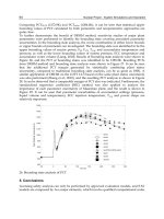
In case of constant temperature pattern the results of the simulation study can be seen in
Fig. 3, which is the part of the examinations where random fluctuations were changed by up
to ± 11K. The number of specimens in the community is permanent and maximum until
Climate Change and Variability148

daily random fluctuation values are between 0 and ±2K. Significant decrease in the number
of specimens depends on the velocity factor of the ecosystem. There is a sudden decrease in
case of a fluctuation of ± 3K in the slower processes while the faster ecosystems react in case
of a random fluctuation of about ± 6K.

Fig. 3. Annual total number of specimens and diversity values versus the daily random
fluctuation in constant temperature environment (The signed plots show the diversity
values.)

There are some local maximums in the diversity function. In case of low fluctuation the
diversity values are low; the largest diversity can be observed in case of medium daily
variation in temperature; in case of large fluctuations, just like in case of the low ones, the
diversity value is quite low. The diversity of the ecosystem which has faster reproductive
ability shows lower local maximum values than that of the slower system in the
experiments.
The degree of the diversity is greater in case of r=0.1 velocity factor than in case of the faster
system. If there is no disturbance, the largest diversity can be observed at 294 K in case of
both speed values. If the fluctuation is between ± 6K and ± 9K, the diversity values are
nearly equally low. In case of the largest variation (± 11K) the degree of the diversity
increases strongly.
In case of constant temperature pattern the Intermediate Disturbance Hypothesis can be
seen well (Fig. 3.). In case of r=1 and T=293 K the specialist (S13) wins the competition when
the random daily fluctuation has rather low values (up to ±1.5K). Then, increasing the
random fluctuation the generalist (T7) is the winner and the transition between the
exchanges of the two type genres shows the local maximum value in case of disturbance,
which is related to IDH. The following competition is between the species T7 and G4 in case
of a fluctuation of about ±2.8K, then between G4 and the super generalist (SG1) in case of

about ±4.5K. These are similar fluctuation values where the IDH can be observed as it can be
seen in Fig. 3.
The shapes of the IDH local maximum curves show similarity in all cases. The maximum
curves increase slowly and decrease steeply. The main reason of this pattern is the
competition between the various species. If the environmental conditions are better for a
genre, the existing genre disappears faster, which explains the steep decrease in the

diversity values after the competition. There are controversies regarding the shape of the
local maximum curves in diversity values versus the random daily fluctuation (Connell,
1978; Elliott et al., 2001).
In case of sine temperature pattern the parameter s
1
was changed during the simulations.
The results of the experiments can be seen in Fig.4. The initial low diversity value increases
as the value of the parameter s
1
grows then decreases again.
There are two peaks in diversity when increasing the amplitude of the annual sine
temperature function (s
1
) in case of low values. The annual total number of specimens is
permanent when s
1
=0…3.5 in case of both velocity parameters, only the diversity value
changes. In case of annual fluctuation (i.e. sine temperature pattern) the Intermediate
Disturbance Hypothesis could be observed as well, and there are two local peaks similarly
to the case of daily fluctuation.


Fig. 4. Annual total numbers of specimens and Shannon diversity values plotted against the
parameter s
1
in case of sine temperature pattern

3.4. Future research
Ecosystems have an important role in the biosphere in development and maintenance of the
equilibrium. Regarding the temperature patterns it is not only the climate environment

which affects the composition of ecosystems but plants also provides a feedback to their
environment through the photosynthesis and respiration in the global carbon cycle.
Community ecological effects of climate change 149

daily random fluctuation values are between 0 and ±2K. Significant decrease in the number
of specimens depends on the velocity factor of the ecosystem. There is a sudden decrease in
case of a fluctuation of ± 3K in the slower processes while the faster ecosystems react in case
of a random fluctuation of about ± 6K.


Fig. 3. Annual total number of specimens and diversity values versus the daily random
fluctuation in constant temperature environment (The signed plots show the diversity
values.)

There are some local maximums in the diversity function. In case of low fluctuation the
diversity values are low; the largest diversity can be observed in case of medium daily
variation in temperature; in case of large fluctuations, just like in case of the low ones, the
diversity value is quite low. The diversity of the ecosystem which has faster reproductive
ability shows lower local maximum values than that of the slower system in the
experiments.
The degree of the diversity is greater in case of r=0.1 velocity factor than in case of the faster
system. If there is no disturbance, the largest diversity can be observed at 294 K in case of
both speed values. If the fluctuation is between ± 6K and ± 9K, the diversity values are
nearly equally low. In case of the largest variation (± 11K) the degree of the diversity
increases strongly.
In case of constant temperature pattern the Intermediate Disturbance Hypothesis can be
seen well (Fig. 3.). In case of r=1 and T=293 K the specialist (S13) wins the competition when
the random daily fluctuation has rather low values (up to ±1.5K). Then, increasing the
random fluctuation the generalist (T7) is the winner and the transition between the
exchanges of the two type genres shows the local maximum value in case of disturbance,

which is related to IDH. The following competition is between the species T7 and G4 in case
of a fluctuation of about ±2.8K, then between G4 and the super generalist (SG1) in case of

about ±4.5K. These are similar fluctuation values where the IDH can be observed as it can be
seen in Fig. 3.
The shapes of the IDH local maximum curves show similarity in all cases. The maximum
curves increase slowly and decrease steeply. The main reason of this pattern is the
competition between the various species. If the environmental conditions are better for a
genre, the existing genre disappears faster, which explains the steep decrease in the
diversity values after the competition. There are controversies regarding the shape of the
local maximum curves in diversity values versus the random daily fluctuation (Connell,
1978; Elliott et al., 2001).
In case of sine temperature pattern the parameter s
1
was changed during the simulations.
The results of the experiments can be seen in Fig.4. The initial low diversity value increases
as the value of the parameter s
1
grows then decreases again.
There are two peaks in diversity when increasing the amplitude of the annual sine
temperature function (s
1
) in case of low values. The annual total number of specimens is
permanent when s
1
=0…3.5 in case of both velocity parameters, only the diversity value
changes. In case of annual fluctuation (i.e. sine temperature pattern) the Intermediate
Disturbance Hypothesis could be observed as well, and there are two local peaks similarly
to the case of daily fluctuation.

Fig. 4. Annual total numbers of specimens and Shannon diversity values plotted against the
parameter s
1
in case of sine temperature pattern

3.4. Future research
Ecosystems have an important role in the biosphere in development and maintenance of the
equilibrium. Regarding the temperature patterns it is not only the climate environment
which affects the composition of ecosystems but plants also provides a feedback to their
environment through the photosynthesis and respiration in the global carbon cycle.
Climate Change and Variability150

The specimens of the ecosystems do not only suffer the change in climate but they can affect
the equilibrium of the biosphere and the composition of the air through the biogeochemical
cycles. There is an opportunity to examine the controlling ability of temperature and climate
with the theoretical ecosystem.
In our further research we would like to examine the feedback of the ecosystem to the
climate. These temperature feedbacks are very important related to DGVM models with
large computation needs (Friedlingstein et al., 2006), but the feedbacks are not estimated
directly. We would like to examine the process of the feedback with PC calculations in order
to answer easy questions.

4. Tactical modelling case study using the example of the phytoplankton
community of a large river (Hungarian stetch of River Danube)
The present subchapter describes the seasonal dynamics of the phytoplankton by means of a
discrete-deterministic model on the basis of the data gathered in the Danube River at Göd
(Hungary). The strategic model, so-called “TEGM” was adapted to field data (tactical
model). The “tactical model” is a simulation model fitted to the observed temperature data
set (Sipkay et al. 2009).

The tactical models could be beneficial if the general functioning of
ecosystems is in the focus (Hufnagel & Gaál 2005; Sipkay et al. 2008a, 2008b; Sipkay et al.
2009; Vadadi et al. 2009).

4.1. Materials and methods
Long-term series of phytoplankton data are available on the river Danube at Göd (1669 rkm)
owing to the continuous record of the Hungarian Danube Research Station of the Hungarian
Academy of Sciences collecting quantitative samples of weekly frequency between 1979 and
2002 (Kiss, 1994). Phytoplankton was sampled from the streamline near the surface and after
processing of samples biomass was calculated (mg l
-1
).
The relatively intensive sampling makes our data capable of being used in simulation
models, which are functions of weather conditions. We assume that temperature is of major
importance when discussing the seasonal dynamics of phytoplankton. What is more, the
reaction curve describing the temperature dependency may be the sum of optimum curves,
because the temperature optimum curves of species or units of phytoplankton and of
biological phenomena determining growth rate are expected to be summed. On the other
hand, the availability of light has also a major influence on the seasonal variation of
phytoplankton abundance; therefore it was taken into account as well. Further biotic and
biotic effects appear within the above-mentioned or hidden.
First, a strategic model, the so-called TEGM (Theoretical Ecosystem Growth Model)
(Drégelyi & Hufnagel, 2009) was used, which involves the temperature optimum curves of
33 theoretical species covering the possible spectrum of temperature. The strategic model of
the theoretical algal community was adapted to field data derived from the river Danube
(tactical model), with respect to the fact that the degree of nutrient oversupply varied
regularly during the study period (Horváth & Tevanné Bartalis, 1999). Assuming that
nutrient oversupply of high magnitude represents a specific environment for
phytoplankton, two sub models were developed, one for the period 1979-1990 with nutrient
oversupply of great magnitude (sub model „A”) and a second one for the period 1991-2002

with lower oversupply (sub model „B”). Either sub model can be described as the linear

combination of 20 theoretical species. These sub models vary slightly in the parameters of
the temperature reaction curves. Biomass (mg l
-1
) of a certain theoretical species is the
function of its biomass measured the day before and the temperature or light coefficient. So
as to define whether temperature or light is the driving force, a minimum function was
applied. Temperature-dependent growth rate can be described with the density function of
normal distribution, whereas light-dependent growth rate includes a term of environmental
sustainability, which was defined with a sine curve representing the scale of light
availability within a year.
The model was run with the data series of climate change scenarios as input parameters
after being fitted (with the Solver optimization program of MS Excel) to the data series of
daily temperatures supplied by the Hungarian Meteorological Service. Data base of the
PRUDENCE EU project (Christensen, 2005) was used, that is, A2 and B2 scenarios proposed
by the IPCC (2007), the daily temperatures of which are specified for the period 2070-2100.
Three data series were used including the A2 and B2 scenarios of the HadCM3 model
developed by the Hadley Centre (HC) and the A2 scenario of the Max Planck Institute
(MPI). Each scenario covers 31 replicates of which we selected 24 so as to compare to
measured data of 24 years between 1979 and 2002. In addition, the effect of linear
temperature rise was tested as follows: each value of the measured temperatures between
1979 and 2002 was increased by 0.5, 1, 1.5 and 2 C, and then the model was run with these
data.
The outcomes were analyzed with statistical methods using the Past software (Hammer et
al., 2001). Yearly total phytoplankton biomass was defined as an indicator; however, it was
calculated as the sum of the monthly average biomass in order to avoid the „side-effect” of
extreme values. One-way ANOVA was applied to demonstrate possible differences between
model outcomes. In order to point out which groups do differ from each other, the post-hoc
Turkey test was used, homogeneity of variance was tested with Levene’s test and standard

deviations were compared with Welch test.

4.2. Results
On the basis of field and simulated data of phytoplankton abundance (Fig. 5), it can be said
that the model fits to the observed values quite well. Yearly total biomass measured in the
field and calculated as the sum of monthly average biomass correlated with the simulated
values (r=0.74).
Phytoplankton biomass varied significantly within outcomes for scenarios and real data
(one-way ANOVA, p<0.001), however, variances did not prove to be homogeneous
(Levene’s test, p<0.001), resulting from the significant differences of standard deviations
(Welch test, p<0.001). Turkey’s pair wise comparisons implied significant differences
between outcomes of the scenario A2 (of MPI) and the others in sub model „A” only
(p<0.05).
Examining the effect of linear temperature rise there were also significant differences
between outputs (one-way ANOVA, p<0.001), similarly, variances were not homogeneous
(Levene’s test, p<0.001), and again, this was interpreted by the significant differences of
standard deviations (Welch test, p<0.001). Turkey’s pair wise comparisons pointed out that
there are significant differences between the outcomes for the period 1979-2002 and
outcomes at a temperature rise of 2 C in case of sub model „A”, furthermore, rises in
temperature of 0.5, 1 and 1.5 C in sub model „A” implied significant differences from the
Community ecological effects of climate change 151

The specimens of the ecosystems do not only suffer the change in climate but they can affect
the equilibrium of the biosphere and the composition of the air through the biogeochemical
cycles. There is an opportunity to examine the controlling ability of temperature and climate
with the theoretical ecosystem.
In our further research we would like to examine the feedback of the ecosystem to the
climate. These temperature feedbacks are very important related to DGVM models with
large computation needs (Friedlingstein et al., 2006), but the feedbacks are not estimated
directly. We would like to examine the process of the feedback with PC calculations in order

to answer easy questions.

4. Tactical modelling case study using the example of the phytoplankton
community of a large river (Hungarian stetch of River Danube)
The present subchapter describes the seasonal dynamics of the phytoplankton by means of a
discrete-deterministic model on the basis of the data gathered in the Danube River at Göd
(Hungary). The strategic model, so-called “TEGM” was adapted to field data (tactical
model). The “tactical model” is a simulation model fitted to the observed temperature data
set (Sipkay et al. 2009).
The tactical models could be beneficial if the general functioning of
ecosystems is in the focus (Hufnagel & Gaál 2005; Sipkay et al. 2008a, 2008b; Sipkay et al.
2009; Vadadi et al. 2009).

4.1. Materials and methods
Long-term series of phytoplankton data are available on the river Danube at Göd (1669 rkm)
owing to the continuous record of the Hungarian Danube Research Station of the Hungarian
Academy of Sciences collecting quantitative samples of weekly frequency between 1979 and
2002 (Kiss, 1994). Phytoplankton was sampled from the streamline near the surface and after
processing of samples biomass was calculated (mg l
-1
).
The relatively intensive sampling makes our data capable of being used in simulation
models, which are functions of weather conditions. We assume that temperature is of major
importance when discussing the seasonal dynamics of phytoplankton. What is more, the
reaction curve describing the temperature dependency may be the sum of optimum curves,
because the temperature optimum curves of species or units of phytoplankton and of
biological phenomena determining growth rate are expected to be summed. On the other
hand, the availability of light has also a major influence on the seasonal variation of
phytoplankton abundance; therefore it was taken into account as well. Further biotic and
biotic effects appear within the above-mentioned or hidden.

First, a strategic model, the so-called TEGM (Theoretical Ecosystem Growth Model)
(Drégelyi & Hufnagel, 2009) was used, which involves the temperature optimum curves of
33 theoretical species covering the possible spectrum of temperature. The strategic model of
the theoretical algal community was adapted to field data derived from the river Danube
(tactical model), with respect to the fact that the degree of nutrient oversupply varied
regularly during the study period (Horváth & Tevanné Bartalis, 1999). Assuming that
nutrient oversupply of high magnitude represents a specific environment for
phytoplankton, two sub models were developed, one for the period 1979-1990 with nutrient
oversupply of great magnitude (sub model „A”) and a second one for the period 1991-2002
with lower oversupply (sub model „B”). Either sub model can be described as the linear

combination of 20 theoretical species. These sub models vary slightly in the parameters of
the temperature reaction curves. Biomass (mg l
-1
) of a certain theoretical species is the
function of its biomass measured the day before and the temperature or light coefficient. So
as to define whether temperature or light is the driving force, a minimum function was
applied. Temperature-dependent growth rate can be described with the density function of
normal distribution, whereas light-dependent growth rate includes a term of environmental
sustainability, which was defined with a sine curve representing the scale of light
availability within a year.
The model was run with the data series of climate change scenarios as input parameters
after being fitted (with the Solver optimization program of MS Excel) to the data series of
daily temperatures supplied by the Hungarian Meteorological Service. Data base of the
PRUDENCE EU project (Christensen, 2005) was used, that is, A2 and B2 scenarios proposed
by the IPCC (2007), the daily temperatures of which are specified for the period 2070-2100.
Three data series were used including the A2 and B2 scenarios of the HadCM3 model
developed by the Hadley Centre (HC) and the A2 scenario of the Max Planck Institute
(MPI). Each scenario covers 31 replicates of which we selected 24 so as to compare to
measured data of 24 years between 1979 and 2002. In addition, the effect of linear

temperature rise was tested as follows: each value of the measured temperatures between
1979 and 2002 was increased by 0.5, 1, 1.5 and 2 C, and then the model was run with these
data.
The outcomes were analyzed with statistical methods using the Past software (Hammer et
al., 2001). Yearly total phytoplankton biomass was defined as an indicator; however, it was
calculated as the sum of the monthly average biomass in order to avoid the „side-effect” of
extreme values. One-way ANOVA was applied to demonstrate possible differences between
model outcomes. In order to point out which groups do differ from each other, the post-hoc
Turkey test was used, homogeneity of variance was tested with Levene’s test and standard
deviations were compared with Welch test.

4.2. Results
On the basis of field and simulated data of phytoplankton abundance (Fig. 5), it can be said
that the model fits to the observed values quite well. Yearly total biomass measured in the
field and calculated as the sum of monthly average biomass correlated with the simulated
values (r=0.74).
Phytoplankton biomass varied significantly within outcomes for scenarios and real data
(one-way ANOVA, p<0.001), however, variances did not prove to be homogeneous
(Levene’s test, p<0.001), resulting from the significant differences of standard deviations
(Welch test, p<0.001). Turkey’s pair wise comparisons implied significant differences
between outcomes of the scenario A2 (of MPI) and the others in sub model „A” only
(p<0.05).
Examining the effect of linear temperature rise there were also significant differences
between outputs (one-way ANOVA, p<0.001), similarly, variances were not homogeneous
(Levene’s test, p<0.001), and again, this was interpreted by the significant differences of
standard deviations (Welch test, p<0.001). Turkey’s pair wise comparisons pointed out that
there are significant differences between the outcomes for the period 1979-2002 and
outcomes at a temperature rise of 2 C in case of sub model „A”, furthermore, rises in
temperature of 0.5, 1 and 1.5 C in sub model „A” implied significant differences from the
Climate Change and Variability152

outcomes of sub model „B” (p<0.05). However, outcomes within sub model „B” showed
large similarity (p=1).

0,00
20,00
40,00
60,00
80,00
100,00
120,00
140,00
0 50 100 150 200 250 300 350 400 450 500 550 600 650 700 750 800 850 900 950 1000 1050 1100 1150
observed
simulated

Fig. 5. The Danubian Phytoplankton Model fitted to the data series of 1979-1990, including
sub model “A” for the period 1979-1990 and sub model “B” for the period 1991-2002.

Fig. 6. shows outputs of means and standard deviations of yearly total biomass of algae on
the basis of monthly averages, from which it is evident that biomass increased largely in
case of scenario A2 (MPI), however, biomass output for the period 1960-1990 increased
notably as well (sub model „A”). Sub model „B” showed minor variations in biomass
compared to model outputs for the period 1979-2002. Nevertheless, standard deviation
showed major increase in each case. Temperature rise of 0.5 C (Fig. 7.) obviously implied
remarkable increase in biomass in case of sub model „A” and negligible changes in case of
sub model „B”.

0
10000

20000
30000
40000
50000
60000
70000
79-'02 Con
(HC)
A2 (HC) B2 (HC) Con
(MPI)
A2
(MPI)
79-'02 Con
(HC)
A2 (HC) B2 (HC) Con
(MPI)
A2
(MPI)
A A A A A A B B B B B B
Mean
St. Dev

Fig. 6. Monthly means and standard deviations of yearly total algal biomass (mg l
-1
) in case
of the model outputs for the period 1979-2002 (based on measured data of temperatures)
compared with outputs of the model run with data series of the climate change scenarios.
Sub models „A” and „B” are presented separately. HC=Hadley Centre; MPI=Max Planck
Institute; A2 and B2 scenarios; Con=control

0
50
100
150
200
250
300
350
400
0 0,5 1 1,5 2 0 0,5 1 1,5 2
A A A A A B B B B B
Mean
St. Dev

Fig. 7. Monthly means and standard deviations of yearly total algal biomass (mg l
-1
) in case
of the model outputs for the period 1979-2002 (based on measured data of temperatures)
compared with outputs of the model run with data series of
linear temperature rises of 0.5
C. Sub models „A” and „B” are presented separately. 0; 0.5; 1; 1.5; 2: degree of linear
temperature rise (
o
C).

4.3. Discussion
Adapting the TEGM model we managed to develop a model that fits to the measured data
quite well. Beyond the indicator of yearly total biomass introduced in the paper, further
indicators can be defined and used in order to get a better understanding of the possible
effects of climate change concerning the phytoplankton in the Danube River.

Interpretation of model outcomes for climate change scenarios is rather difficult. Comparing
the model outcomes for the control period 1960-1990 with the outcomes for the case of
applying the observed temperature data of 1979-2002 as input parameters, there are
remarkable differences. Major variation within data series of certain climate change
scenarios may account for the increased standard deviations observed in the model outputs.
Sub model „B”, assuming minor nutrient oversupply, implied minor increase in biomass
and variation within scenarios was of minor importance.
In case of linear temperature rise a clear answer is received: the more drastic warming
results in greater abundance of phytoplankton if only the environment rich in nutrients is
assumed (as it was experienced between 1979 and 1990). Moderate nutrient supply does not
favour algae even if temperatures increase by 2 C, thus biomass is not expected to increase
notably. All these draw attention to the increased hazard of nutrient loading in rivers: global
warming brings more drastic changes to nutrient rich environments.
Global warming can influence the tropic state and primary productivity of inland waters in
a very fundamental way (Lofgren, 2002). Bacterial metabolism, rate of nutrient cycling and
algal production all increase with rising temperatures (Klapper, 1991). Generally, climate
change together with anthropogenic pollution enhances eutrophication (Klapper, 1991;
Adrian et al., 1995). Several studies derived their findings from models forecasting increased
phytoplankton abundance mostly through rising trophy (Mooij et al., 2007; Elliot et al., 2005;
Komatsu et al., 2007). These are in line with our results of linear temperature rise, but only
in case of high nutrient load. Global warming does not have so severe effects on
phytoplankton biomass under conditions of lower nutrient load.
Looking at the variation in phytoplankton biomass only is not relevant enough in order to
explore the effects of climate change. Freshwater food webs show rather characteristic
seasonal dynamics, thus the effect of climate is the function of the season (Straile, 2005). If
Community ecological effects of climate change 153

outcomes of sub model „B” (p<0.05). However, outcomes within sub model „B” showed
large similarity (p=1).

0,00
20,00
40,00
60,00
80,00
100,00
120,00
140,00
0 50 100 150 200 250 300 350 400 450 500 550 600 650 700 750 800 850 900 950 1000 1050 1100 1150
observed
simulated

Fig. 5. The Danubian Phytoplankton Model fitted to the data series of 1979-1990, including
sub model “A” for the period 1979-1990 and sub model “B” for the period 1991-2002.

Fig. 6. shows outputs of means and standard deviations of yearly total biomass of algae on
the basis of monthly averages, from which it is evident that biomass increased largely in
case of scenario A2 (MPI), however, biomass output for the period 1960-1990 increased
notably as well (sub model „A”). Sub model „B” showed minor variations in biomass
compared to model outputs for the period 1979-2002. Nevertheless, standard deviation
showed major increase in each case. Temperature rise of 0.5 C (Fig. 7.) obviously implied
remarkable increase in biomass in case of sub model „A” and negligible changes in case of
sub model „B”.

0
10000
20000
30000
40000
50000

60000
70000
79-'02 Con
(HC)
A2 (HC) B2 (HC) Con
(MPI)
A2
(MPI)
79-'02 Con
(HC)
A2 (HC) B2 (HC) Con
(MPI)
A2
(MPI)
A A A A A A B B B B B B
Mean
St. Dev

Fig. 6. Monthly means and standard deviations of yearly total algal biomass (mg l
-1
) in case
of the model outputs for the period 1979-2002 (based on measured data of temperatures)
compared with outputs of the model run with data series of the climate change scenarios.
Sub models „A” and „B” are presented separately. HC=Hadley Centre; MPI=Max Planck
Institute; A2 and B2 scenarios; Con=control

0
50
100
150

200
250
300
350
400
0 0,5 1 1,5 2 0 0,5 1 1,5 2
A A A A A B B B B B
Mean
St. Dev

Fig. 7. Monthly means and standard deviations of yearly total algal biomass (mg l
-1
) in case
of the model outputs for the period 1979-2002 (based on measured data of temperatures)
compared with outputs of the model run with data series of
linear temperature rises of 0.5
C. Sub models „A” and „B” are presented separately. 0; 0.5; 1; 1.5; 2: degree of linear
temperature rise (
o
C).

4.3. Discussion
Adapting the TEGM model we managed to develop a model that fits to the measured data
quite well. Beyond the indicator of yearly total biomass introduced in the paper, further
indicators can be defined and used in order to get a better understanding of the possible
effects of climate change concerning the phytoplankton in the Danube River.
Interpretation of model outcomes for climate change scenarios is rather difficult. Comparing
the model outcomes for the control period 1960-1990 with the outcomes for the case of
applying the observed temperature data of 1979-2002 as input parameters, there are
remarkable differences. Major variation within data series of certain climate change

scenarios may account for the increased standard deviations observed in the model outputs.
Sub model „B”, assuming minor nutrient oversupply, implied minor increase in biomass
and variation within scenarios was of minor importance.
In case of linear temperature rise a clear answer is received: the more drastic warming
results in greater abundance of phytoplankton if only the environment rich in nutrients is
assumed (as it was experienced between 1979 and 1990). Moderate nutrient supply does not
favour algae even if temperatures increase by 2 C, thus biomass is not expected to increase
notably. All these draw attention to the increased hazard of nutrient loading in rivers: global
warming brings more drastic changes to nutrient rich environments.
Global warming can influence the tropic state and primary productivity of inland waters in
a very fundamental way (Lofgren, 2002). Bacterial metabolism, rate of nutrient cycling and
algal production all increase with rising temperatures (Klapper, 1991). Generally, climate
change together with anthropogenic pollution enhances eutrophication (Klapper, 1991;
Adrian et al., 1995). Several studies derived their findings from models forecasting increased
phytoplankton abundance mostly through rising trophy (Mooij et al., 2007; Elliot et al., 2005;
Komatsu et al., 2007). These are in line with our results of linear temperature rise, but only
in case of high nutrient load. Global warming does not have so severe effects on
phytoplankton biomass under conditions of lower nutrient load.
Looking at the variation in phytoplankton biomass only is not relevant enough in order to
explore the effects of climate change. Freshwater food webs show rather characteristic
seasonal dynamics, thus the effect of climate is the function of the season (Straile, 2005). If
Climate Change and Variability154

we are interested in the phenomena within a year, further indicators can be introduced into
the model. Such indicators include those showing the day of population peak (blooms)
within a year or those representing 50% of the yearly total biomass. Some day the model
will be able to provide us with an insight into the effects of global warming from a broader
perspective by taking advantage of new indicators.

5. Spatial climatic analogy (SCA)

With the method of the spatial climatic analogy we search for regions which have the same
climate at present as the scenarios indicate for the future. With the spatial analogy we can
make the climate scenarios easier to understand. In this research the analogue regions for
Debrecen, which is an agriculturally important region in Hungary, were examined.
According to the result we can say, in line with international results, that our climate will be
similar to that of regions south of Hungary. This shifting will be 250-450 km in the next
decades (2011-2040) and it could be 450-650 km in the middle of the century and maybe
there will be no spatial analogues in Europe by the end of the century. Different methods
were used to calculate the analogues, but they indicate the same regions. These analogue
regions are North-Serbia, the region Vojvodina, South Romania and North Bulgaria in the
next decades, and South Bulgaria and North Greece in the middle of the century. We
developed the inverse analogy method, with the help of which we can search for regions
which will have the same climate in future as there is in Debrecen at present. If we accept
the results of spatial analogy, we can identify the analogue regions and compare their data.
Data were collected from the databases EUROSTATs and CORINE. We collected all the data
on land use, crops and natural vegetation. These data show that land use may become more
diverse, which is advantageous in adaptation to climate change. The ratio of forests and
pastures may become higher. In the next decade’s maize and wheat will be more important
because climatic conditions will become better for them (because of the “corn belt”).
The tendency of a potential global climate change is still not obvious, but the most accepted
models predict warming and increase in extreme weather events. As the climate change has
an overall impact on human health, natural systems and agricultural production and also
has socio-economic impacts, it is very important to predict potential changes to have enough
time for appropriate decision-making. Analogue scenarios involve the use of past warm
climates as scenarios of future climate (temporal analogue scenario) and the use of the
current climate in another (usually warmer) location as a scenario of future climate in the
study area (spatial analogue scenario). Our aim was to find spatial analogues to describe the
potential future climate of Hungary. However, we must note that climate depends also on
other effects, especially on elevation, topography and storm track conditions, which cannot
be considered in this kind of analysis.

5.1. Materials and methods of spatial climatic analogy
Climate scenarios can be defined as relevant and adequate pictures of how the climate may
look like in the future. Our work is based on General Circulation Models (GCMs)
downscaled to Debrecen, an important centre of agricultural production in Hungary and we
used the method of geographical analogies to explain the results. We used different GCM
scenarios (HadCM3 A1FI, B2), the IPCC CRU Global Climate dataset and the Hungarian
meteorological database for 30 years (1961-1990). To find the analogues, monthly data were

used. Monthly temperature averages and precipitation sums were used for 4 different time
periods, for the base period 1961-1990 and for the future periods 2010-2019, 2020-2029, 2020-
2039 and 2040-2069. To calculate and find the analogue regions we used the SCA method,
which was improved by us.




12
1
12
1
i
ijidj
TTEMPT

(3)






12
1
)(112
1
i
iji
iji
dj
PPRECa
PPREC
P

(4)
djT
Tk
Tj
eI




(5)
djP
Pk
Pj
eI


)1(



(6)
PjTjj
IICMI



(7)
Where:
• j: grid point identity number (j=1-31143)
• i: month (i=1-12)
• TEMP
ji
: monthly mean temperature of the grid point j for the base period
• T
i
: monthly mean temperature of the grid point j for the scenario
• PREC
ji
: monthly precipitation of the grid point j for the base period
• P
i
: monthly precipitation of the grid point j for the scenario
• T
dj
: average of temperature differences
• P
dj
: average of precipitation differences

• I
Tj
: similarity of the climate for the scenario in temperature
• I
Pj
: similarity of the climate for the scenario in precipitation
• CMI
j
: „Composite Match Index”, if CMI>90%, we can call the grid point the
analogue for the scenario

5.2. Analogue regions
First we looked for the analogue regions for the base period. We found that we got back our
regions after looking for the analogues in the future. We found that the analogue regions are
south of Debrecen. This climate shifting was the same in case of different scenarios because
in the first decades they do not differ very much but we can see more differences in the
middle of the century. Finally, we defined the analogue regions for the scenarios and time
periods. We found that the climatic shifting would be 250-450 km in the next decades and
450- 650 km by the middle of the century. Unfortunately we could not find any similar
regions for the end of the century, but some analogues can be found in North Africa.








Community ecological effects of climate change 155

we are interested in the phenomena within a year, further indicators can be introduced into
the model. Such indicators include those showing the day of population peak (blooms)
within a year or those representing 50% of the yearly total biomass. Some day the model
will be able to provide us with an insight into the effects of global warming from a broader
perspective by taking advantage of new indicators.

5. Spatial climatic analogy (SCA)
With the method of the spatial climatic analogy we search for regions which have the same
climate at present as the scenarios indicate for the future. With the spatial analogy we can
make the climate scenarios easier to understand. In this research the analogue regions for
Debrecen, which is an agriculturally important region in Hungary, were examined.
According to the result we can say, in line with international results, that our climate will be
similar to that of regions south of Hungary. This shifting will be 250-450 km in the next
decades (2011-2040) and it could be 450-650 km in the middle of the century and maybe
there will be no spatial analogues in Europe by the end of the century. Different methods
were used to calculate the analogues, but they indicate the same regions. These analogue
regions are North-Serbia, the region Vojvodina, South Romania and North Bulgaria in the
next decades, and South Bulgaria and North Greece in the middle of the century. We
developed the inverse analogy method, with the help of which we can search for regions
which will have the same climate in future as there is in Debrecen at present. If we accept
the results of spatial analogy, we can identify the analogue regions and compare their data.
Data were collected from the databases EUROSTATs and CORINE. We collected all the data
on land use, crops and natural vegetation. These data show that land use may become more
diverse, which is advantageous in adaptation to climate change. The ratio of forests and
pastures may become higher. In the next decade’s maize and wheat will be more important
because climatic conditions will become better for them (because of the “corn belt”).
The tendency of a potential global climate change is still not obvious, but the most accepted
models predict warming and increase in extreme weather events. As the climate change has
an overall impact on human health, natural systems and agricultural production and also
has socio-economic impacts, it is very important to predict potential changes to have enough

time for appropriate decision-making. Analogue scenarios involve the use of past warm
climates as scenarios of future climate (temporal analogue scenario) and the use of the
current climate in another (usually warmer) location as a scenario of future climate in the
study area (spatial analogue scenario). Our aim was to find spatial analogues to describe the
potential future climate of Hungary. However, we must note that climate depends also on
other effects, especially on elevation, topography and storm track conditions, which cannot
be considered in this kind of analysis.

5.1. Materials and methods of spatial climatic analogy
Climate scenarios can be defined as relevant and adequate pictures of how the climate may
look like in the future. Our work is based on General Circulation Models (GCMs)
downscaled to Debrecen, an important centre of agricultural production in Hungary and we
used the method of geographical analogies to explain the results. We used different GCM
scenarios (HadCM3 A1FI, B2), the IPCC CRU Global Climate dataset and the Hungarian
meteorological database for 30 years (1961-1990). To find the analogues, monthly data were

used. Monthly temperature averages and precipitation sums were used for 4 different time
periods, for the base period 1961-1990 and for the future periods 2010-2019, 2020-2029, 2020-
2039 and 2040-2069. To calculate and find the analogue regions we used the SCA method,
which was improved by us.




12
1
12
1
i
ijidj

TTEMPT

(3)





12
1
)(112
1
i
iji
iji
dj
PPRECa
PPREC
P

(4)
djT
Tk
Tj
eI




(5)

djP
Pk
Pj
eI


)1(


(6)
PjTjj
IICMI 

(7)
Where:
• j: grid point identity number (j=1-31143)
• i: month (i=1-12)
• TEMP
ji
: monthly mean temperature of the grid point j for the base period
• T
i
: monthly mean temperature of the grid point j for the scenario
• PREC
ji
: monthly precipitation of the grid point j for the base period
• P
i
: monthly precipitation of the grid point j for the scenario
• T

dj
: average of temperature differences
• P
dj
: average of precipitation differences
• I
Tj
: similarity of the climate for the scenario in temperature
• I
Pj
: similarity of the climate for the scenario in precipitation
• CMI
j
: „Composite Match Index”, if CMI>90%, we can call the grid point the
analogue for the scenario

5.2. Analogue regions
First we looked for the analogue regions for the base period. We found that we got back our
regions after looking for the analogues in the future. We found that the analogue regions are
south of Debrecen. This climate shifting was the same in case of different scenarios because
in the first decades they do not differ very much but we can see more differences in the
middle of the century. Finally, we defined the analogue regions for the scenarios and time
periods. We found that the climatic shifting would be 250-450 km in the next decades and
450- 650 km by the middle of the century. Unfortunately we could not find any similar
regions for the end of the century, but some analogues can be found in North Africa.

Climate Change and Variability156

TIME Base period
1961-
1990

For validating the method,
analogues for the observed climate
were calculated. As a result we got
back the region of Debrecen.
A1F1 B2
2010-
2019


2020-
2029


2030-
2039


2040-
2069

Fig. 8. Analogue regions in the next decades and in case of different climate scenarios for
Debrecen

We developed a new method to find inverse analogue regions; these are the regions the
climate of which will be similar to that of our study area in the future. We found a same
shifting to the north. These analogue regions are in Poland (Fig. 9.) and were defined for the
scenario A2.

Similarity
(%)
2011-2040 2041-2070


Analogue regions: PL11, PL43, PL41

Analogue regions: PL61, PL12, PL31
Fig. 9. Analogue regions in the next decades and in case of different climate scenarios for
Debrecen

It can be seen that analogue regions are south-east of Debrecen about 250-450 km away but
later this distance is larger. The analogue regions are Vojvodina in Serbia as well as the
RO04 (Sud-Vest) and the RO03 (Sud) NUTS regions in Romania. For further analyses only
these regions were taken into consideration (Fig. 10.). We calculated the diversity of
croplands and the land use and we found opposite changes. While the diversity of
croplands is lower than in Hungary, the diversity of land use is higher. It is mostly because
of the main crops. The ratio of wheat and maize is higher in the South, just because the
climatic conditions are better for them. Meanwhile the yield is lower; it is more economical
to use these crops because the better conditions necessitate less agronomic techniques.

Diversity of the croplands. In the analogue
regions the diversity is lower, so the
structure of the croplands in Hungary will
probably change, too.

Diversity of the land use types is higher in
the analogue regions, but it could be
caused by the topography as well.
Community ecological effects of climate change 157

TIME Base period
1961-
1990

For validating the method,
analogues for the observed climate
were calculated. As a result we got
back the region of Debrecen.
A1F1 B2
2010-
2019


2020-
2029


2030-
2039

2040-
2069


Fig. 8. Analogue regions in the next decades and in case of different climate scenarios for
Debrecen

We developed a new method to find inverse analogue regions; these are the regions the
climate of which will be similar to that of our study area in the future. We found a same
shifting to the north. These analogue regions are in Poland (Fig. 9.) and were defined for the
scenario A2.

Similarity
(%)
2011-2040 2041-2070


Analogue regions: PL11, PL43, PL41

Analogue regions: PL61, PL12, PL31
Fig. 9. Analogue regions in the next decades and in case of different climate scenarios for
Debrecen

It can be seen that analogue regions are south-east of Debrecen about 250-450 km away but
later this distance is larger. The analogue regions are Vojvodina in Serbia as well as the
RO04 (Sud-Vest) and the RO03 (Sud) NUTS regions in Romania. For further analyses only
these regions were taken into consideration (Fig. 10.). We calculated the diversity of
croplands and the land use and we found opposite changes. While the diversity of
croplands is lower than in Hungary, the diversity of land use is higher. It is mostly because

of the main crops. The ratio of wheat and maize is higher in the South, just because the
climatic conditions are better for them. Meanwhile the yield is lower; it is more economical
to use these crops because the better conditions necessitate less agronomic techniques.


Diversity of the croplands. In the analogue
regions the diversity is lower, so the
structure of the croplands in Hungary will
probably change, too.

Diversity of the land use types is higher in
the analogue regions, but it could be
caused by the topography as well.
Climate Change and Variability158


Ratio of the maize fields in the arable land
is higher in the analogue regions than in
Hungary. Climate change could have a
positive effect on the Hungarian maize
production, too.

The ratio of the wheat fields in the
analogue regions is similar to the present
situation in Hungary. Climate change may
not have an effect on it.
Fig. 10. Land use and cropland ratio of the analogue regions

5.3. Discussion
Debrecen, the basic object of our calculations, is an important centre of agricultural

production in Hungary, so we would like to interpret the results in this aspect.
Climate, especially temperature and precipitation, basically determines agricultural
production. Results show that in Hungary we have to count on an increase in temperature
and decrease in precipitation. The possible future climate predicted by the scenarios will be
similar to the present climate of South-Southeast Europe. Of course climate depends also on
other effects, especially on elevation, topography and storm-track conditions, which could
not be considered in this kind of analysis. However, the method of spatial analogies seems
to be a good tool to understand and interpret the results of the GCM scenarios and the
effects of climate change, so we want to go ahead in this research. This method and
additional data on the analogue regions can provide information on the impacts of climate
change on ecosystems or on agricultural production, such as the changes in land use,
cropping system or yields and on the possibilities for disappearing or introducing new
crops or weeds and pests into an area.
Increase in mean annual temperatures in our region, if limited to two or three degrees, can
generally be expected to extend the growing season. In case of crops (or animals), where
phonological phases depend on accumulated heat units, the phenophases can become
shorter. Whether crops respond to higher temperatures with an increase or decrease in yield
depends on whether their yield is currently strongly limited by insufficient warmth or the
temperature is near or little above the optimum. In Central Europe, where temperatures are
near the optimum under current climatic conditions, increases in temperature would
probably lead to decreased yields in case of several crops. Increased temperature could be
favourable for example for pepper and grapes; however, it is unfavourable for green peas
and potato. Decrease in precipitation could be a great limiting factor in agriculture.
If we accept the results of the GCMs, according to the A1FI scenario for the period
2011-2040, the analogue regions of Debrecen will be the Vojvodina region in Serbia and
South Romania. It means a shifting of about 250-450 km south, which corresponds to other
international results.
The detailed analyses of the analogue regions can help us to adapt to the changing climate.
From the analogue regions we should collect all kind of available ecological, agricultural,

economic, social and public sanitation data. We can study what kind of problems there are,
and what the solutions are. We can learn from there how to solve the possible problems and
develop strategies. This would be a good base for further research and an important base for
decision makers.
With the method of spatial analogy we can build a new way of knowledge transfer from
where we can learn adaptation techniques and to where we can transfer our knowledge.

6. References
Adrian, R., Deneke, R., Mischke, U., Stellmacher, R., Lederer, P. (1995). A long-term study of
the Heilingensee (1975–1992). Evidence for effects of climatic change on the
dynamics of eutrophied lake ecosystems. Archiv fur Hydrobiol 133: 315–337.
Allan, J.D., Palmer, M., Poff, N.L. (2005). Climate change and freshwater ecosystems. In:
Lovejoy, T.E., Hannah, L. (eds): Climate change and biodiversity. Yale University Press,
New Haven, CT, pp. 274–295.
Baltz, D.M., Moyle, P.B. (1993). Invasion resistance to introduced species by a native
assemblage of California stream fishes. Ecol Appl 3: 246–255.
Christensen, J. H. (2005). Prediction of Regional scenarios and Uncertainties for Defining
European Climate change risks and Effects. Final Report. DMI, Copenhagen.
Clements, F. E. (1905). Research methods in ecology. University Publishing. Lincoln, Nebraska,
USA.
Connell, J. H. (1978). Diversity in tropical rain forests and coral reefs. Science, 199., 1302 –
1310, 0036-8075
Drégelyi-Kiss, Á. & Hufnagel, L. (2010). Effects of temperature-climate patterns on the
production of some competitive species on grounds of modelling. Environmental
Modeling & Assessment, Doi :10.1007/s10666-009-9216-4, 1573-2967
Drégelyi-Kiss, Á. & Hufnagel, L. (2009). Simulations of Theoretical Ecosystem Growth
Model (TEGM) during various climate conditions. Applied Ecology and
Environmental Research, 7(1)., 71-78, 1785-0037
Drégelyi-Kiss, Á., Drégelyi-Kiss, G. & Hufnagel, L. (2008). Ecosystems as climate controllers
– biotic feedbacks (a review). Applied Ecology and Environmental Research, 6(2)., 111-

135, 1785-0037
Elliott, J. A., Irish, A. E. & Reynolds, C. S. (2001). The effects of vertical mixing on a
phytoplankton community: a modelling approach to the intermediate disturbance
hypothesis. Freshwater Biology, 46., 1291–1297, 0046-5070
Elliott, J. A., Thackeray, S. J., Huntingford, C. & Jones, R.G. (2005). Combining a regional
climate model with a phytoplankton community model to predict future changes in
phytoplankton in lakes. Freshwater Biology 50: 1404-1411.
Elton, C.S. (1927). Animal ecology. Sidgwick and Jackson, London, GB 207 pp.
Felföldy, L (1981). Water environmental sciences. Mezőgazdasági Kiadó, Budapest [in
Hungarian]
Ficke, A.D., Myrick, C.A., Hansen, L.J. (2007). Potential impacts of global climate change on
freshwater fisheries. Rev. Fish. Biol. Fisheries 17: 581-613.
Community ecological effects of climate change 159


Ratio of the maize fields in the arable land
is higher in the analogue regions than in
Hungary. Climate change could have a
positive effect on the Hungarian maize
production, too.

The ratio of the wheat fields in the
analogue regions is similar to the present
situation in Hungary. Climate change may
not have an effect on it.
Fig. 10. Land use and cropland ratio of the analogue regions

5.3. Discussion
Debrecen, the basic object of our calculations, is an important centre of agricultural
production in Hungary, so we would like to interpret the results in this aspect.

Climate, especially temperature and precipitation, basically determines agricultural
production. Results show that in Hungary we have to count on an increase in temperature
and decrease in precipitation. The possible future climate predicted by the scenarios will be
similar to the present climate of South-Southeast Europe. Of course climate depends also on
other effects, especially on elevation, topography and storm-track conditions, which could
not be considered in this kind of analysis. However, the method of spatial analogies seems
to be a good tool to understand and interpret the results of the GCM scenarios and the
effects of climate change, so we want to go ahead in this research. This method and
additional data on the analogue regions can provide information on the impacts of climate
change on ecosystems or on agricultural production, such as the changes in land use,
cropping system or yields and on the possibilities for disappearing or introducing new
crops or weeds and pests into an area.
Increase in mean annual temperatures in our region, if limited to two or three degrees, can
generally be expected to extend the growing season. In case of crops (or animals), where
phonological phases depend on accumulated heat units, the phenophases can become
shorter. Whether crops respond to higher temperatures with an increase or decrease in yield
depends on whether their yield is currently strongly limited by insufficient warmth or the
temperature is near or little above the optimum. In Central Europe, where temperatures are
near the optimum under current climatic conditions, increases in temperature would
probably lead to decreased yields in case of several crops. Increased temperature could be
favourable for example for pepper and grapes; however, it is unfavourable for green peas
and potato. Decrease in precipitation could be a great limiting factor in agriculture.
If we accept the results of the GCMs, according to the A1FI scenario for the period
2011-2040, the analogue regions of Debrecen will be the Vojvodina region in Serbia and
South Romania. It means a shifting of about 250-450 km south, which corresponds to other
international results.
The detailed analyses of the analogue regions can help us to adapt to the changing climate.
From the analogue regions we should collect all kind of available ecological, agricultural,

economic, social and public sanitation data. We can study what kind of problems there are,

and what the solutions are. We can learn from there how to solve the possible problems and
develop strategies. This would be a good base for further research and an important base for
decision makers.
With the method of spatial analogy we can build a new way of knowledge transfer from
where we can learn adaptation techniques and to where we can transfer our knowledge.

6. References
Adrian, R., Deneke, R., Mischke, U., Stellmacher, R., Lederer, P. (1995). A long-term study of
the Heilingensee (1975–1992). Evidence for effects of climatic change on the
dynamics of eutrophied lake ecosystems. Archiv fur Hydrobiol 133: 315–337.
Allan, J.D., Palmer, M., Poff, N.L. (2005). Climate change and freshwater ecosystems. In:
Lovejoy, T.E., Hannah, L. (eds): Climate change and biodiversity. Yale University Press,
New Haven, CT, pp. 274–295.
Baltz, D.M., Moyle, P.B. (1993). Invasion resistance to introduced species by a native
assemblage of California stream fishes. Ecol Appl 3: 246–255.
Christensen, J. H. (2005). Prediction of Regional scenarios and Uncertainties for Defining
European Climate change risks and Effects. Final Report. DMI, Copenhagen.
Clements, F. E. (1905). Research methods in ecology. University Publishing. Lincoln, Nebraska,
USA.
Connell, J. H. (1978). Diversity in tropical rain forests and coral reefs. Science, 199., 1302 –
1310, 0036-8075
Drégelyi-Kiss, Á. & Hufnagel, L. (2010). Effects of temperature-climate patterns on the
production of some competitive species on grounds of modelling. Environmental
Modeling & Assessment, Doi :10.1007/s10666-009-9216-4, 1573-2967
Drégelyi-Kiss, Á. & Hufnagel, L. (2009). Simulations of Theoretical Ecosystem Growth
Model (TEGM) during various climate conditions. Applied Ecology and
Environmental Research, 7(1)., 71-78, 1785-0037
Drégelyi-Kiss, Á., Drégelyi-Kiss, G. & Hufnagel, L. (2008). Ecosystems as climate controllers
– biotic feedbacks (a review). Applied Ecology and Environmental Research, 6(2)., 111-
135, 1785-0037

Elliott, J. A., Irish, A. E. & Reynolds, C. S. (2001). The effects of vertical mixing on a
phytoplankton community: a modelling approach to the intermediate disturbance
hypothesis. Freshwater Biology, 46., 1291–1297, 0046-5070
Elliott, J. A., Thackeray, S. J., Huntingford, C. & Jones, R.G. (2005). Combining a regional
climate model with a phytoplankton community model to predict future changes in
phytoplankton in lakes. Freshwater Biology 50: 1404-1411.
Elton, C.S. (1927). Animal ecology. Sidgwick and Jackson, London, GB 207 pp.
Felföldy, L (1981). Water environmental sciences. Mezőgazdasági Kiadó, Budapest [in
Hungarian]
Ficke, A.D., Myrick, C.A., Hansen, L.J. (2007). Potential impacts of global climate change on
freshwater fisheries. Rev. Fish. Biol. Fisheries 17: 581-613.
Climate Change and Variability160

Fischlin, A., G.F. Midgley, J.T. Price, R. Leemans, B. Gopal, C. Turley, M.D.A. Rounsevell,
O.P. Dube, J. Tarazona, A.A. Velichko (2007). Ecosystems, their properties, goods,
and services. In: Climate Change. (2007). Impacts, Adaptation and Vulnerability.
Contribution of Working Group II to the Fourth Assessment Report of the
Intergovernmental Panel on Climate Change, M.L. Parry, O.F. Canziani, J.P. Palutikof,
P.J. van der Linden and C.E. Hanson, Eds., Cambridge University Press,
Cambridge, pp. 211 – 272
Friedlingstein, P., Cox, P. M., Betts, R. A., Bopp, L., von Bloh, W., Brovkin, V., Cadule, P.,
Doney, S., Eby, M., Fung, I., Bala, G., John, J., Jones, C. D., Joos, F., Kato, T.,
Kawamiya, M., Knorr, W., Lindsay, K., Matthews, H. D., Raddatz, T., Rayner, P.,
Reick, C., Roeckner, E., Schnitzler, K. G., Schnur, R., Strassmann, K., Weaver, A. J.,
Yoshikawa, C. & Zeng, N. (2006). Climate-Carbon Cycle feedback analysis: Results
from the C4MIP model incomparison, Journal of Climate, 19., 3337-3353, 0894-8755
Fulbright, T. E. (1996). Viewpoint: a theoretical basis for planning woody plant control to
maintain species diversity. Journal of Range Management, 49., 554– 559, 0022-409X
Gleason, Henry A. (1926). The Individualistic Concept of the Plant Association. Bulletin of the
Torrey Botanical Club 53: 7-26

Haffner, G. D., Harris, G. P. & Jarai, M. K. (1980). Physical variability and phytoplankton
communities. III. Vertical structure in phytoplankton populations. Archiv für
Hydrobiologie, 89., 363 – 381, 0003-9136
Hammer, O., Harper, D. A. T. & Ryan, P. D. (2001). PAST: Paleontological statistics software
package for education and data nalysis. Paleontologia Electronica, 4(1), 9.
Horváth, L. & Tevanné Bartalis, É. (1999). A vízkémiai viszonyok jellemzése a Duna Rajka-
Szob közötti szakaszán. Vízügyi Közlemények. 81: 54-85.(in Hungarian)
Hufnagel L., Sipkay Cs., Drégelyi-Kiss Á., Farkas E., Türei D. , Gergócs V., Petrányi G.,
Baksa A., Gimesi L., Eppich B., Dede L., Horváth L. (2008). Interactions between the
processes of climate change, bio-diversity and community ecology. In Climate
Change: Environment, Risk, Society. Harnos Zs., Csete L. (Eds.), 227-264. Szaktudás
Kiadó Ház, ISBN 978-963-9736-87-0, Budapest (in Hungarian)
Hufnagel, L. & Gaál, M. (2005): Seasonal dynamic pattern analysis service of climate change
research. Applied Ecology and Environmental Research 3(1): 79–132.
Hufnagel, L., Drégelyi-Kiss, G. & Drégelyi-Kiss, Á. (2010). The effect of the reproductivity’s
velocity on the biodiversity of a theoretical ecosystem, Applied Ecology and
Environmental Research, in press, 1785-0037
IPCC (2007). The Fourth Assessment Report “Climate Change 2007” Cambridge University
Press 2008 ISBN-13:9780521705974
Kalff, J. (2000). Limnology. Prentice Hall, Upper Saddle River, New Jersey.
Kiss, K. T. 1994. Trophic level and eutrophication of the River Danube in Hungary.
Verh.Internat.Verein.Limnol. 25: 1688-1691.
Klapper, H. (1991). Control of eutrophication in Inland waters. Ellis Horwood Ltd., West Sussex,
UK.
Komatsu, E., Fukushima, T. & Harasawa, H. (2007). A modeling approach to forecast the
effect of long-term climate change on lake water quality. Ecological Modelling 209:
351-366.

Köck, G., Triendl, M., Hofer, R. (1996). Seasonal patterns of metal accumulation in Arctic
char (Salvelinus alpinus) from an oligotrophic Alpine lake related to temperature.

Can J Fisher Aqua Sci 53: 780–786.
Lofgren, B.M. (2002). Global warming influences on water levels, ice, and chemical and
biological cycles in lakes: some examples. In: McGinn NA (ed) Fisheries in a changing
climate. American Fisheries Society, Bethesda, MD, pp. 15–22.
Lovelock J.E (1972). "Gaia as seen through the atmosphere". Atmospheric Environment 6 (8):
579–580.
Lovelock J.E (1990). "Hands up for the Gaia hypothesis". Nature 344 (6262): 100–2.
MacLeod, J.C., Pessah, E. (1973). Temperature effects on mercury accumulation, toxicity, and
metabolic rate in rainbow trout (Salmo gairdneri). J Fisher Res Board Can 30: 485–
492.
Magnuson, J.J. (2002.a). Future of adapting to climate change and variability. In: McGinn NA
(ed) Fisheries in a changing climate. American Fisheries Society, Bethesda, MD, pp.
283–287.
Matthews, W.J., Marsh-Matthews, E. (2003). Effects of drought on fish across axes of space,
time and ecological complexity. Freshwater Biol 48: 1232–1253.
Mitchell T.D., Carter T.R., Jones P.D., Hulme,M., New, M., (2003). A comprehensive set of
high-resolution grids of monthly climate for Europe and the globe: the observed
record (1901-2000) and 16 scenarios (2001-2100). Journal of Climate
Mooij, W.M., Janse, J.H., Domis, L.N., Hülsmann, S., Ibelings, B.W. (2007): Predicting the
effect of climate change on temperate shallow lakes with the ecosystem model
PCLake. Hydrobiologia 584:443–454.
Murty, A.S. (1986.a). Toxicity of pesticides to Fish. I. CRC Press, Boca Raton, FL.
Murty, A.S. (1986.b). Toxicity of pesticides to Fish. II. CRC Press, Boca Raton, FL.
Nussey, G., van Vuren, J.H.J., du Preez, H.H. (1996). Acute toxicity of copper on juvenile
Mozambique tilapia, Oreochromis mossambicus (Cichlidae), at different
temperatures. S Afr J Wildlife Res 26: 47–55.
Olrik, K. & Nauwerck, A. (1993). Stress and disturbance in the phytoplankton community of
a shallow, hypertrophic lake. Hydrobiologia, 249., 15 – 24, 0018-8158
Padisák, J. (1998). Sudden and gradual responses of phytoplankton to global climate change:
case studies from two large, shallow lakes (Balaton, Hungary and the

Neusiedlersee, Austria/Hungary). In Management of Lakes and Reservoirs during
Global Change. George, D. G, Jones, J. G, Puncochar, P., Reynolds, C. S. & Sutcliffe, D. W.
(Eds.), 111–125, Kluwer Academic Publishers, ISBN-0-7923-5055-3, Dordrecht,
Boston, London.
Pianka, E. R. (1974). Niche overlap and diffuse competition, Proceedings of the National
Academy of Sciences of the United States of America, 71., 2141-2145, 0027-8424
Poff, N.L., Brinson, M.M., Day, J.W. (2002). Aquatic ecosystem & Climate change. Potential
impacts on inland freshwater and coastal wetland ecosystems in the United States. Pew
Center on Globa Climate Change. pp. 44.
Reynolds, C. S. (2006). The ecology of phytoplankton. Cambridge University Press, ISBN-13
978-0-521-84413-0, Cambridge
Community ecological effects of climate change 161

Fischlin, A., G.F. Midgley, J.T. Price, R. Leemans, B. Gopal, C. Turley, M.D.A. Rounsevell,
O.P. Dube, J. Tarazona, A.A. Velichko (2007). Ecosystems, their properties, goods,
and services. In: Climate Change. (2007). Impacts, Adaptation and Vulnerability.
Contribution of Working Group II to the Fourth Assessment Report of the
Intergovernmental Panel on Climate Change, M.L. Parry, O.F. Canziani, J.P. Palutikof,
P.J. van der Linden and C.E. Hanson, Eds., Cambridge University Press,
Cambridge, pp. 211 – 272
Friedlingstein, P., Cox, P. M., Betts, R. A., Bopp, L., von Bloh, W., Brovkin, V., Cadule, P.,
Doney, S., Eby, M., Fung, I., Bala, G., John, J., Jones, C. D., Joos, F., Kato, T.,
Kawamiya, M., Knorr, W., Lindsay, K., Matthews, H. D., Raddatz, T., Rayner, P.,
Reick, C., Roeckner, E., Schnitzler, K. G., Schnur, R., Strassmann, K., Weaver, A. J.,
Yoshikawa, C. & Zeng, N. (2006). Climate-Carbon Cycle feedback analysis: Results
from the C4MIP model incomparison, Journal of Climate, 19., 3337-3353, 0894-8755
Fulbright, T. E. (1996). Viewpoint: a theoretical basis for planning woody plant control to
maintain species diversity. Journal of Range Management, 49., 554– 559, 0022-409X
Gleason, Henry A. (1926). The Individualistic Concept of the Plant Association. Bulletin of the
Torrey Botanical Club 53: 7-26

Haffner, G. D., Harris, G. P. & Jarai, M. K. (1980). Physical variability and phytoplankton
communities. III. Vertical structure in phytoplankton populations. Archiv für
Hydrobiologie, 89., 363 – 381, 0003-9136
Hammer, O., Harper, D. A. T. & Ryan, P. D. (2001). PAST: Paleontological statistics software
package for education and data nalysis. Paleontologia Electronica, 4(1), 9.
Horváth, L. & Tevanné Bartalis, É. (1999). A vízkémiai viszonyok jellemzése a Duna Rajka-
Szob közötti szakaszán. Vízügyi Közlemények. 81: 54-85.(in Hungarian)
Hufnagel L., Sipkay Cs., Drégelyi-Kiss Á., Farkas E., Türei D. , Gergócs V., Petrányi G.,
Baksa A., Gimesi L., Eppich B., Dede L., Horváth L. (2008). Interactions between the
processes of climate change, bio-diversity and community ecology. In Climate
Change: Environment, Risk, Society. Harnos Zs., Csete L. (Eds.), 227-264. Szaktudás
Kiadó Ház, ISBN 978-963-9736-87-0, Budapest (in Hungarian)
Hufnagel, L. & Gaál, M. (2005): Seasonal dynamic pattern analysis service of climate change
research. Applied Ecology and Environmental Research 3(1): 79–132.
Hufnagel, L., Drégelyi-Kiss, G. & Drégelyi-Kiss, Á. (2010). The effect of the reproductivity’s
velocity on the biodiversity of a theoretical ecosystem, Applied Ecology and
Environmental Research, in press, 1785-0037
IPCC (2007). The Fourth Assessment Report “Climate Change 2007” Cambridge University
Press 2008 ISBN-13:9780521705974
Kalff, J. (2000). Limnology. Prentice Hall, Upper Saddle River, New Jersey.
Kiss, K. T. 1994. Trophic level and eutrophication of the River Danube in Hungary.
Verh.Internat.Verein.Limnol. 25: 1688-1691.
Klapper, H. (1991). Control of eutrophication in Inland waters. Ellis Horwood Ltd., West Sussex,
UK.
Komatsu, E., Fukushima, T. & Harasawa, H. (2007). A modeling approach to forecast the
effect of long-term climate change on lake water quality. Ecological Modelling 209:
351-366.

Köck, G., Triendl, M., Hofer, R. (1996). Seasonal patterns of metal accumulation in Arctic
char (Salvelinus alpinus) from an oligotrophic Alpine lake related to temperature.

Can J Fisher Aqua Sci 53: 780–786.
Lofgren, B.M. (2002). Global warming influences on water levels, ice, and chemical and
biological cycles in lakes: some examples. In: McGinn NA (ed) Fisheries in a changing
climate. American Fisheries Society, Bethesda, MD, pp. 15–22.
Lovelock J.E (1972). "Gaia as seen through the atmosphere". Atmospheric Environment 6 (8):
579–580.
Lovelock J.E (1990). "Hands up for the Gaia hypothesis". Nature 344 (6262): 100–2.
MacLeod, J.C., Pessah, E. (1973). Temperature effects on mercury accumulation, toxicity, and
metabolic rate in rainbow trout (Salmo gairdneri). J Fisher Res Board Can 30: 485–
492.
Magnuson, J.J. (2002.a). Future of adapting to climate change and variability. In: McGinn NA
(ed) Fisheries in a changing climate. American Fisheries Society, Bethesda, MD, pp.
283–287.
Matthews, W.J., Marsh-Matthews, E. (2003). Effects of drought on fish across axes of space,
time and ecological complexity. Freshwater Biol 48: 1232–1253.
Mitchell T.D., Carter T.R., Jones P.D., Hulme,M., New, M., (2003). A comprehensive set of
high-resolution grids of monthly climate for Europe and the globe: the observed
record (1901-2000) and 16 scenarios (2001-2100). Journal of Climate
Mooij, W.M., Janse, J.H., Domis, L.N., Hülsmann, S., Ibelings, B.W. (2007): Predicting the
effect of climate change on temperate shallow lakes with the ecosystem model
PCLake. Hydrobiologia 584:443–454.
Murty, A.S. (1986.a). Toxicity of pesticides to Fish. I. CRC Press, Boca Raton, FL.
Murty, A.S. (1986.b). Toxicity of pesticides to Fish. II. CRC Press, Boca Raton, FL.
Nussey, G., van Vuren, J.H.J., du Preez, H.H. (1996). Acute toxicity of copper on juvenile
Mozambique tilapia, Oreochromis mossambicus (Cichlidae), at different
temperatures. S Afr J Wildlife Res 26: 47–55.
Olrik, K. & Nauwerck, A. (1993). Stress and disturbance in the phytoplankton community of
a shallow, hypertrophic lake. Hydrobiologia, 249., 15 – 24, 0018-8158
Padisák, J. (1998). Sudden and gradual responses of phytoplankton to global climate change:
case studies from two large, shallow lakes (Balaton, Hungary and the

Neusiedlersee, Austria/Hungary). In Management of Lakes and Reservoirs during
Global Change. George, D. G, Jones, J. G, Puncochar, P., Reynolds, C. S. & Sutcliffe, D. W.
(Eds.), 111–125, Kluwer Academic Publishers, ISBN-0-7923-5055-3, Dordrecht,
Boston, London.
Pianka, E. R. (1974). Niche overlap and diffuse competition, Proceedings of the National
Academy of Sciences of the United States of America, 71., 2141-2145, 0027-8424
Poff, N.L., Brinson, M.M., Day, J.W. (2002). Aquatic ecosystem & Climate change. Potential
impacts on inland freshwater and coastal wetland ecosystems in the United States. Pew
Center on Globa Climate Change. pp. 44.
Reynolds, C. S. (2006). The ecology of phytoplankton. Cambridge University Press, ISBN-13
978-0-521-84413-0, Cambridge