Fuel Injection Part 6 ppt

Effect of injector nozzle holes on diesel engine performance 93



Fig. 21. Unburned fuel in cylinder of
injector nozzle 9 holes
Fig. 22. Unburned fuel in cylinder of
injector nozzle 10 holes

6. Effect of Injector Nozzle Holes on Engine Performance
The simulation result on engine performance effect of injector fuel nozzle holes number and
geometries in indicated power, indicated torque and indicated specific fuel consumption
(ISFC) of engine are shown in Figure 23 – 25. The injector fuel nozzle holes orifice diameter
and injector nozzle holes numbers effect on indicated power, indicated torque and ISFC
performance of direct-injection diesel engine was shown from the simulation model running
output. An aerodynamic interaction and turbulence seem to have competing effects on
spray breakup as the fuel nozzle holes orifice diameter decreases. The fuel drop size
decreases if the fuel nozzle holes orifice diameter is decreases with a decreasing quantitative
effect for a given set of jet conditions.

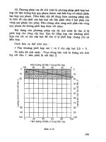
Indicated Torque Effect of Fuel Nozzle Holes Number
0
5
10
15
20
25
30
35
40
45

0 500 1000 1500 2000 2500 3000 3500 4000 4500
Engine Speed (rpm)
Indicated Torque (N-m
)
Nozzle 1 hole Nozzle 2 holes Nozzle 3 holes Nozzle 4 holes Nozzle 5 holes
Nozzle 6 holes Nozzle 7 holes Nozzle 8 holes Nozzle 9 holes Nozzle 10holes

Fig. 23.
Effect of fuel nozzle holes on indicated torque of diesel engine

Indicated Power Effect of Fuel Nozzle Holes Number
0
1
2
3
4
5
6
7
8
9
10
0 500 1000 1500 2000 2500 3000 3500 4000 4500
Engine Speed (rpm)
Indicated Power (kW
)
Nozzle 1 hole Nozzle 2 holes Nozzle 3 holes Nozzle 4 holes Nozzle 5 holes
Nozzle 6 holes Nozzle 7 holes Nozzle 8 holes Nozzle 9 holes Nozzle 10holes

Fig. 24.

Effect of fuel nozzle holes on indicated power of diesel engine

ISFC Effect of Fuel Nozzle Holes Number
1100
1600
2100
2600
3100
3600
4100
4600
0 500 1000 1500 2000 2500 3000 3500 4000 4500
Engine Speed (rpm)
ISFC (g/kW-h
)
Nozzle 1 hole Nozzle 2 holes Nozzle 3 holes Nozzle 4 holes Nozzle 5 holes
Nozzle 6 holes Nozzle 7 holes Nozzle 8 holes Nozzle 9 holes Nozzle 10 holes

Fig. 25.
Effect of fuel nozzle holes on ISFC of diesel engine
Fuel Injection94

Fuel-air mixing increases as the fuel nozzle holes orifice diameter fuel nozzle holes
decreases. Also soot incandescence is observed to decrease as the amount of fuel-air
premixing upstream of the lift-off length increases. This can be a significant advantage for
small orifice nozzles hole. However, multiple holes orifices diameter required to meet the
desired mass flow rate as orifice diameter decreases. In this case, the orifices diameter need
to placed with appropriate spacing and directions in order to avoid interference among
adjacent sprays. The empirical correlations generally predict smaller drop size, slower
penetrating speed and smaller spray cone angles as the orifice diameter decreases, however

the predicted values were different for different relation. All of the nozzles have examined
and the results are shown that the five holes nozzle provided the best results for indicted
torque, indicated power and ISFC in any different engine speed in simulation.

7. Conclusion
All of the injector nozzle holes have examined and the results are shown that the seven holes
nozzle have provided the best burning result for the fuel in-cylinder burned in any different
engine speeds and the best burning is in low speed engine. In engine performance effect, all
of the nozzles have examined and the five holes nozzle provided the best result in indicted
power, indicated torque and ISFC in any different engine speeds.

8. References

Baik, Seunghyun. (2001). Development of Micro-Diesel Injector Nozzles Via MEMS
Technology and Effects on Spray Characteristics, PhD Dissertation, University of
Wisconsin-Madison, USA.
Bakar, R.A., Semin., Ismail, A.R. and Ali, Ismail., 2008. Computational Simulation of Fuel
Nozzle Multi Holes Geometries Effect on Direct Injection Diesel Engine
Performance Using GT-POWER. American Journal of Applied Sciences 5 (2): 110-116.
Baumgarter, Carsten. (2006). Mixture Formation in Internal Combustion Engines, Spinger
Berlin.
Gamma Technologies, (2004). GT-POWER User’s Manual 6.1, Gamma Technologies Inc.
Ganesan, V. (1999). Internal Combustion Engines 2
nd
Edition, Tata McGraw-Hill, New Delhi,
India.
Heywood, J.B. (1988). Internal Combustion Engine Fundamentals - Second Edition, McGraw-
Hill, Singapore.
Kowalewicz, Andrzej., 1984. Combustion System of High-Speed Piston I.C. Engines,
Wydawnictwa Komunikacji i Lacznosci, Warszawa.

Semin and Bakar, R.A. (2007). Nozzle Holes Effect on Unburned Fuel in Injected and In-
Cylinder Fuel of Four Stroke Direct Injection Diesel Engine. Presearch Journal of
Applied Sciences 2 (11): 1165-1169.
Semin., Bakar, R.A. and Ismail, A.R. (2007). Effect Of Engine Performance For Four-Stroke
Diesel Engine Using Simulation,

Proceeding The 5
th
International Conference On
Numerical Analysis in Engineering, Padang-West Sumatera, Indonesia.
Stone, Richard. (1997). Introduction to Internal Combustion Engines-Second Edition, SAE Inc,
USA.

Accurate modelling of an injector for common rail systems 95
Accurate modelling of an injector for common rail systems
Claudio Dongiovanni and Marco Coppo
1
Accurate Modelling of an Injector
for Common Rail Systems
Claudio Dongiovanni
Politecnico di Torino, Dipartimento di Energetica,
Corso Duca degli Abruzzi 24, 10129, Torino
Italy
Marco Coppo
O.M.T. S.p.A., Via Ferrero 67/A, 10090, Cascine Vica Rivoli
Italy
1. Introduction
It is well known that the injection system plays a leading role in achieving high diesel engine
performance; the introduction of the common rail fuel injection system (Boehner & Kumel,
1997; Schommers et al., 2000; Stumpp & Ricco, 1996) represented a major evolutionary step

that allowed the diesel engine to reach high efficiency and low emissions in a wide range of
load conditions.
Many experimental works show the positive effects of splitting the injection process in several
pilot, main and post injections on the reduction of noise, soot and NOx emission (Badami et al.,
2002; Brusca et al., 2002; Henelin et al., 2002; Park et al., 2004; Schmid et al., 2002). In addition,
the success of engine downsizing (Beatrice et al., 2003) and homogeneous charge combustion
engines (HCCI) (Canakci & Reitz, 2004; Yamane & Shimamoto, 2002) is deeply connected with
the injection system performance and injection strategy.
However, the development of a high performance common rail injection system requires a
considerable investment in terms of time, as well as money, due to the need of fine tuning
the operation of its components and, in particular, of the electronic fuel injector. In this light,
numerical simulation models represent a crucial tool for reducing the amount of experiments
needed to reach the final product configuration.
Many common-rail injector models are reported in the literature. (Amoia et al., 1997; Bianchi
et al., 2000; Brusca et al., 2002; Catalano et al., 2002; Ficarella et al., 1999; Payri et al., 2004).
One of the older common-rail injector model was presented in (Amoia et al., 1997) and suc-
cessively improved and employed for the analysis of the instability phenomena due to the
control valve behaviour (Ficarella et al., 1999). An important input parameter in this model
was the magnetic attraction force in the control valve dynamic model. This was calculated
interpolating the experimental curve between driving current and magnetic force measured
at fixed control valve positions. The discharge coefficient of the feeding and discharge control
volume holes were determined and the authors asserted that the discharge hole operates, with
the exception of short transients, under cavitating flow conditions at every working pressure,
6
Fuel Injection96
but this was not confirmed by (Coppo & Dongiovanni, 2007). Furthermore, the deformation
of the stressed injector mechanical components was not taken into account. In (Bianchi et al.,
2000) the electromagnetic attraction force was evaluated by means of a phenomenological
model. The force was considered directly proportional to the square of the magnetic flux and
the proportionality constant was experimentally determined under stationary conditions. The

elastic deformation of the moving injector components were considered, but the injector body
was treated as a rigid body. The models in (Brusca et al., 2002; Catalano et al., 2002) were
very simple models. The aims in (Catalano et al., 2002) were to prove that pressure drops
in an injection system are mainly caused by dynamic effects rather than friction losses and
to analyse new common-rail injection system configurations in which the wave propagation
phenomenon was used to increase the injection pressure. The model in (Brusca et al., 2002)
was developed in the AMESim environment and its goal was to give the boundary conditions
to a 3D-CFD code for spray simulation. Payri et al. (2004) report a model developed in the
AMESim environment too, and suggest silicone moulds as an interesting tool for characteris-
ing valve and nozzle hole geometry.
A common-rail injector model employs three sub-models (electrical, hydraulic and mechan-
ical) to describe all the phenomena that govern injector operation. Before one can use the
model to estimate the effects of little adjustments or little geometrical modifications on the
system performance, it is fundamental to validate the predictions of all the sub-models in the
whole range of possible working conditions.
In the following sections of this chapter every sub-model will be thoroughly presented and it
will be shown how its parameters can be evaluated by means of theoretical or experimental
analysis. The focus will be placed on the electronic injector, as this component is the heart of
any common rail system
2. Mathematical model
The injector considered in this investigation is a standard Bosch UNIJET unit (Fig. 1) of the
common-rail type used in car engines, but the study methodology that will be discussed can
be easily adapted to injectors manufactured by other companies.
The definition of a mathematical model always begins with a thorough analysis of the parts
that make up the component to be modelled. Once geometrical details and functional rela-
tionships between parts are acquired and understood they can be described in terms of math-
ematical relationships. For the injector, this leads to the definition of hydraulic, mechanical,
and electromagnetic models.
2.1 Hydraulic Model
Fig. 2 shows the equivalent hydraulic circuit of the injector, drawn following ISO 1219 stan-

dards. Continuous lines represent the main connecting ducts, while dashed lines represent
pilot and vent connections. The hydraulic parts of the injector that have limited spatial ex-
tension are modelled with ideal components such as uniform pressure chambers and laminar
or turbulent hydraulic resistances, according to a zero-dimensional approach. The internal
hole connecting injector inlet with the nozzle delivery chamber (as well as the pipe connect-
ing the injector to the rail or the rail to the high pressure pump) are modelled according to
a one-dimensional approach because wave propagation phenomena in these parts play an
important role in determining injector performance.
Fig. 3a shows the control valve and the relative equivalent hydraulic circuit. R
A
and R
Z
are the hydraulic resistances used for modelling flow through control-volume orifices A (dis-
1. Control valve pin 4. C-shaped connecting pin and anchor
2. Pin guide and upper stop 5. Control volume feeding (Z) hole
3. Control valve anchor 6. Control volume discharge (A) hole
Fig. 1. Standard Bosch UNIJET injector
charge) and Z (feeding), respectively. The variable resistance R
AZ
models the flow between
chambers C
dZ
and C
uA
, taking into account the effect of the control piston position on the
actual flow area between the aforementioned chambers. The solenoid control valve V
c
is rep-
resented using its standard symbol, which shows the forces that act in the opening (one gen-
erated by the current I flowing through the solenoid, the other by the pressure in the chamber

C
dA
) and closing direction (spring force).
Fig. 3b illustrates the control piston and nozzle along with the relative equivalent hydraulic
circuit. The needle valve V
n
is represented with all the actions governing the needle motion,
such as pressures acting on different surface areas, force applied by the control piston and
spring force. The chamber C
D
models the nozzle delivery volume, C
S
is the sac volume,
whereas the hydraulic resistance R
hi
represents the i-th nozzle hole through which fuel is
injected in the combustion chamber C
e
. The control piston model considers two different
surface areas on one side, so as to take into account the different contribution of pressure in
the chambers C
uA
and C
dZ
to the total force applied in the needle valve closing direction.
Leakages both between control valve and piston and between needle and its liner are mod-
elled by means of the resistances R
P
and R
n

respectively, and the resulting flow, which is
collected in chamber C
T
(the annular chamber around the control piston), is then returned to
Accurate modelling of an injector for common rail systems 97
but this was not confirmed by (Coppo & Dongiovanni, 2007). Furthermore, the deformation
of the stressed injector mechanical components was not taken into account. In (Bianchi et al.,
2000) the electromagnetic attraction force was evaluated by means of a phenomenological
model. The force was considered directly proportional to the square of the magnetic flux and
the proportionality constant was experimentally determined under stationary conditions. The
elastic deformation of the moving injector components were considered, but the injector body
was treated as a rigid body. The models in (Brusca et al., 2002; Catalano et al., 2002) were
very simple models. The aims in (Catalano et al., 2002) were to prove that pressure drops
in an injection system are mainly caused by dynamic effects rather than friction losses and
to analyse new common-rail injection system configurations in which the wave propagation
phenomenon was used to increase the injection pressure. The model in (Brusca et al., 2002)
was developed in the AMESim environment and its goal was to give the boundary conditions
to a 3D-CFD code for spray simulation. Payri et al. (2004) report a model developed in the
AMESim environment too, and suggest silicone moulds as an interesting tool for characteris-
ing valve and nozzle hole geometry.
A common-rail injector model employs three sub-models (electrical, hydraulic and mechan-
ical) to describe all the phenomena that govern injector operation. Before one can use the
model to estimate the effects of little adjustments or little geometrical modifications on the
system performance, it is fundamental to validate the predictions of all the sub-models in the
whole range of possible working conditions.
In the following sections of this chapter every sub-model will be thoroughly presented and it
will be shown how its parameters can be evaluated by means of theoretical or experimental
analysis. The focus will be placed on the electronic injector, as this component is the heart of
any common rail system
2. Mathematical model

The injector considered in this investigation is a standard Bosch UNIJET unit (Fig. 1) of the
common-rail type used in car engines, but the study methodology that will be discussed can
be easily adapted to injectors manufactured by other companies.
The definition of a mathematical model always begins with a thorough analysis of the parts
that make up the component to be modelled. Once geometrical details and functional rela-
tionships between parts are acquired and understood they can be described in terms of math-
ematical relationships. For the injector, this leads to the definition of hydraulic, mechanical,
and electromagnetic models.
2.1 Hydraulic Model
Fig. 2 shows the equivalent hydraulic circuit of the injector, drawn following ISO 1219 stan-
dards. Continuous lines represent the main connecting ducts, while dashed lines represent
pilot and vent connections. The hydraulic parts of the injector that have limited spatial ex-
tension are modelled with ideal components such as uniform pressure chambers and laminar
or turbulent hydraulic resistances, according to a zero-dimensional approach. The internal
hole connecting injector inlet with the nozzle delivery chamber (as well as the pipe connect-
ing the injector to the rail or the rail to the high pressure pump) are modelled according to
a one-dimensional approach because wave propagation phenomena in these parts play an
important role in determining injector performance.
Fig. 3a shows the control valve and the relative equivalent hydraulic circuit. R
A
and R
Z
are the hydraulic resistances used for modelling flow through control-volume orifices A (dis-
1. Control valve pin 4. C-shaped connecting pin and anchor
2. Pin guide and upper stop 5. Control volume feeding (Z) hole
3. Control valve anchor 6. Control volume discharge (A) hole
Fig. 1. Standard Bosch UNIJET injector
charge) and Z (feeding), respectively. The variable resistance R
AZ
models the flow between

chambers C
dZ
and C
uA
, taking into account the effect of the control piston position on the
actual flow area between the aforementioned chambers. The solenoid control valve V
c
is rep-
resented using its standard symbol, which shows the forces that act in the opening (one gen-
erated by the current I flowing through the solenoid, the other by the pressure in the chamber
C
dA
) and closing direction (spring force).
Fig. 3b illustrates the control piston and nozzle along with the relative equivalent hydraulic
circuit. The needle valve V
n
is represented with all the actions governing the needle motion,
such as pressures acting on different surface areas, force applied by the control piston and
spring force. The chamber C
D
models the nozzle delivery volume, C
S
is the sac volume,
whereas the hydraulic resistance R
hi
represents the i-th nozzle hole through which fuel is
injected in the combustion chamber C
e
. The control piston model considers two different
surface areas on one side, so as to take into account the different contribution of pressure in

the chambers C
uA
and C
dZ
to the total force applied in the needle valve closing direction.
Leakages both between control valve and piston and between needle and its liner are mod-
elled by means of the resistances R
P
and R
n
respectively, and the resulting flow, which is
collected in chamber C
T
(the annular chamber around the control piston), is then returned to
Fuel Injection98
Fig. 2. Injection equivalent hydraulic circuit
tank after passing through a small opening, modelled with the resistance R
T
, between control
valve and injector body.
2.1.1 Zero-dimensional hydraulic model
The continuity and compressibility equation is written for every chamber in the model
∑
Q =
V
E
l
dp
dt
+

dV
dt
(1)
where
∑
Q is the net flow-rate coming into the chamber,
(V/E
l
)(dp/dt) the rate of increase of
the fluid volume in the chamber due to the fluid compressibility and
(dV/dt) the deformation
rate of the chamber volume.
Fluid leakages occurring between coupled mechanical elements in relative motion (e.g. nee-
dle and its liner, or control piston and control valve body) are modelled using laminar flow
hydraulic resistances, characterized by a flow rate proportional to the pressure drop ∆p across
the element
Q
= K
L
∆p (2)
where the theoretical value of K
L
for an annulus shaped cross-section flow area can be ob-
tained by
K
L
=
πd
m
g

3
12lρν
(3)
In case of eccentric annulus shaped cross-section flow area, Eq. 3 gives an underestimation of
the leakage flow rate that can be as low as one third of the real one (White, 1991).
(a) Control valve (b) Needle and control piston
Fig. 3. Injection equivalent hydraulic circuit
Furthermore, the leakage flow rate, Equations 2 and 3, depends on the third power of the
radial gap g. At high pressure the material deformation strongly affects the gap entity and
its value is not constant along the gap length l because pressure decreases in the gap when
approaching the low pressure side (Ganser, 2000). In order to take into account these effects
on the leakage flow rate, the value of K
L
has to be experimentally evaluated in the real injector
working conditions.
Turbulent flow is assumed to occur in control volume feeding and discharge holes, in nozzle
holes and in the needle-seat opening passage. As a result, according to Bernoulli’s law, the
flow rate through these orifices is proportional to the square root of the pressure drop, ∆p,
across the orifice, namely,
Q
= µA

2∆p
ρ
(4)
The flow model through these orifices plays a fundamental role in the simulation of the injec-
tor behavior in its whole operation field, so the evaluation of the µ factor is extremely impor-
tant.
2.1.2 Hole A and Z discharge coefficient
The discharge coefficient of control volume orifices A and Z is evaluated according to the

model proposed in (Von Kuensberg Sarre et al., 1999). This considers four flow regimes inside
the hole: laminar, turbulent, reattaching and fully cavitating.
Neglecting cavitation occurrence, a preliminary estimation of the hole discharge coefficient
can be obtained as follows
1
µ
=

K
I
+ f
l
d
+ 1 (5)
where K
I
is the inlet loss coefficient, which is a function of the hole inlet geometry (Munson
et al., 1990), l is the hole axial length, d is the hole diameter, and f is the wall friction coefficient,
evaluated as
f
= MAX

64
Re
, 0.316 Re
0.25

(6)
Accurate modelling of an injector for common rail systems 99
Fig. 2. Injection equivalent hydraulic circuit

tank after passing through a small opening, modelled with the resistance R
T
, between control
valve and injector body.
2.1.1 Zero-dimensional hydraulic model
The continuity and compressibility equation is written for every chamber in the model
∑
Q =
V
E
l
dp
dt
+
dV
dt
(1)
where
∑
Q is the net flow-rate coming into the chamber,
(V/E
l
)(dp/dt) the rate of increase of
the fluid volume in the chamber due to the fluid compressibility and
(dV/dt) the deformation
rate of the chamber volume.
Fluid leakages occurring between coupled mechanical elements in relative motion (e.g. nee-
dle and its liner, or control piston and control valve body) are modelled using laminar flow
hydraulic resistances, characterized by a flow rate proportional to the pressure drop ∆p across
the element

Q
= K
L
∆p (2)
where the theoretical value of K
L
for an annulus shaped cross-section flow area can be ob-
tained by
K
L
=
πd
m
g
3
12lρν
(3)
In case of eccentric annulus shaped cross-section flow area, Eq. 3 gives an underestimation of
the leakage flow rate that can be as low as one third of the real one (White, 1991).
(a) Control valve (b) Needle and control piston
Fig. 3. Injection equivalent hydraulic circuit
Furthermore, the leakage flow rate, Equations 2 and 3, depends on the third power of the
radial gap g. At high pressure the material deformation strongly affects the gap entity and
its value is not constant along the gap length l because pressure decreases in the gap when
approaching the low pressure side (Ganser, 2000). In order to take into account these effects
on the leakage flow rate, the value of K
L
has to be experimentally evaluated in the real injector
working conditions.
Turbulent flow is assumed to occur in control volume feeding and discharge holes, in nozzle

holes and in the needle-seat opening passage. As a result, according to Bernoulli’s law, the
flow rate through these orifices is proportional to the square root of the pressure drop, ∆p,
across the orifice, namely,
Q
= µA

2∆p
ρ
(4)
The flow model through these orifices plays a fundamental role in the simulation of the injec-
tor behavior in its whole operation field, so the evaluation of the µ factor is extremely impor-
tant.
2.1.2 Hole A and Z discharge coefficient
The discharge coefficient of control volume orifices A and Z is evaluated according to the
model proposed in (Von Kuensberg Sarre et al., 1999). This considers four flow regimes inside
the hole: laminar, turbulent, reattaching and fully cavitating.
Neglecting cavitation occurrence, a preliminary estimation of the hole discharge coefficient
can be obtained as follows
1
µ
=

K
I
+ f
l
d
+ 1 (5)
where K
I

is the inlet loss coefficient, which is a function of the hole inlet geometry (Munson
et al., 1990), l is the hole axial length, d is the hole diameter, and f is the wall friction coefficient,
evaluated as
f
= MAX

64
Re
, 0.316 Re
0.25

(6)
Fuel Injection100
where Re stands for the Reynolds number.
The ratio between the cross section area of the vena contracta and the geometrical hole area,
µ
vc
, can be evaluated with the relation:
1
µ
2
vc
=
1
µ
2
vc
0
− 11.4
r

d
(7)
where µ
vc
0
= 0.61 (Munson et al., 1990) and r is the fillet radius of the hole inlet.
It follows that the pressure in the vena contracta can be estimated as
p
vc
= p
u
−
ρ
l
2

Q
Aµ
vc

2
(8)
If the pressure in the vena contracta (p
vc
) is higher then the oil vapor pressure (p
v
), cavita-
tion does not occur and the value of the hole discharge coefficient is given by Equation 5.
Otherwise, cavitation occurs and the discharge coefficient is evaluated according to
µ

= µ
vc

p
u
− p
v
p
u
− p
d
(9)
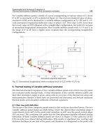
The geometrical profile of the hole inlet plays a crucial role in determining, or avoiding, the
onset of cavitation in the flow. In turn, the occurrence of cavitation strongly affects the flow
rate through the orifice, as can be seen in Figure 4, which shows two trends of predicted flow
rate (Q/Q
0
) in function of pressure drop (∆p = p
u
− p
d
) through holes with the same diameter
and length, but characterized by two different values of the r/d ratio (0.2 and 0.02), when p
u
is kept constant and p
d
is progressively decreased. In absence of cavitation, (r/d = 0.2), the
relation between flow rate and pressure drop is monotonic while, if cavitation occurs (r/d
=
0.02), the hole experiences a decrease in flow rate as pressure drop is further increased. This

behavior agrees with experimental data reported in the literature (Lefebvre, 1989).
Fig. 4. Predicted flow through an orifice in presence/absence of cavitation
Obviously, such behavior would reflect strongly on the injector performance if the control vol-
ume holes happened to cavitate in some working conditions. Therefore, in order to accurately
model the injector operation, it is necessary to accurately measure the geometrical profile of
the control volume holes A and Z; by means of silicone moulds, as proposed by (Payri et al.,
2004), it is possible to acquire an image of the hole shape details, as shown in Figure 5.
(a) A hole (b) Z hole
Fig. 5. Moulds of the control valve holes
By means of imaging techniques it is possible to measure the r/d ratio of the hole under
investigation. Table 1 reports the results obtained for the injector under investigation. The
value of K
I
, in Equation 5, is a function of r/d only (Von Kuensberg Sarre et al., 1999) and,
hence, easily obtainable.
Knowing that during production a hydro-erosion process is applied to make sure that, under
steady flow conditions, all the holes yield the same flow rate, it is possible to define an itera-
tive procedure to calculate the hole diameter using the discharge coefficient model presented
above and the the steady flow rate value. This approach is preferrable to the estimation of the
hole diameter with imaging techniques because it yields a result that is consistent with the
discharge coefficient model used.
r/d K
I
d [µm]
Hole A 0.23
±5% 0.033 280±2%
Hole Z 0.22
±5% 0.034 249±2%
Table 1. Characteristics of control volume holes
In the control valve used in our experiments, under a pressure drop of 10 MPa, with a back

pressure of 4 MPa, the holes A and Z yielded 6.5
± 0.2 cm
3
/s and 5.3 ± 0.2 cm
3
/s, respectively.
With these values it is possible to calculate the most probable diameter of the control volume
holes, as reported in Table 1. It is worth noting that the precision with which the diameters
were evaluated was higher than that of the optical technique used for evaluating the shape of
the control volume holes. This resulted from the fact that K
I
shows little dependence on r/d
when the latter assumes values as high as those measured. As a consequence, the experimen-
tal uncertainty in the diameter estimation is mainly originated from the uncertainty given on
the stationary flow rate through the orifices.
Accurate modelling of an injector for common rail systems 101
where Re stands for the Reynolds number.
The ratio between the cross section area of the vena contracta and the geometrical hole area,
µ
vc
, can be evaluated with the relation:
1
µ
2
vc
=
1
µ
2
vc

0
− 11.4
r
d
(7)
where µ
vc
0
= 0.61 (Munson et al., 1990) and r is the fillet radius of the hole inlet.
It follows that the pressure in the vena contracta can be estimated as
p
vc
= p
u
−
ρ
l
2

Q
Aµ
vc

2
(8)
If the pressure in the vena contracta (p
vc
) is higher then the oil vapor pressure (p
v
), cavita-

tion does not occur and the value of the hole discharge coefficient is given by Equation 5.
Otherwise, cavitation occurs and the discharge coefficient is evaluated according to
µ
= µ
vc

p
u
− p
v
p
u
− p
d
(9)
The geometrical profile of the hole inlet plays a crucial role in determining, or avoiding, the
onset of cavitation in the flow. In turn, the occurrence of cavitation strongly affects the flow
rate through the orifice, as can be seen in Figure 4, which shows two trends of predicted flow
rate (Q/Q
0
) in function of pressure drop (∆p = p
u
− p
d
) through holes with the same diameter
and length, but characterized by two different values of the r/d ratio (0.2 and 0.02), when p
u
is kept constant and p
d
is progressively decreased. In absence of cavitation, (r/d = 0.2), the

relation between flow rate and pressure drop is monotonic while, if cavitation occurs (r/d
=
0.02), the hole experiences a decrease in flow rate as pressure drop is further increased. This
behavior agrees with experimental data reported in the literature (Lefebvre, 1989).
Fig. 4. Predicted flow through an orifice in presence/absence of cavitation
Obviously, such behavior would reflect strongly on the injector performance if the control vol-
ume holes happened to cavitate in some working conditions. Therefore, in order to accurately
model the injector operation, it is necessary to accurately measure the geometrical profile of
the control volume holes A and Z; by means of silicone moulds, as proposed by (Payri et al.,
2004), it is possible to acquire an image of the hole shape details, as shown in Figure 5.
(a) A hole (b) Z hole
Fig. 5. Moulds of the control valve holes
By means of imaging techniques it is possible to measure the r/d ratio of the hole under
investigation. Table 1 reports the results obtained for the injector under investigation. The
value of K
I
, in Equation 5, is a function of r/d only (Von Kuensberg Sarre et al., 1999) and,
hence, easily obtainable.
Knowing that during production a hydro-erosion process is applied to make sure that, under
steady flow conditions, all the holes yield the same flow rate, it is possible to define an itera-
tive procedure to calculate the hole diameter using the discharge coefficient model presented
above and the the steady flow rate value. This approach is preferrable to the estimation of the
hole diameter with imaging techniques because it yields a result that is consistent with the
discharge coefficient model used.
r/d K
I
d [µm]
Hole A 0.23±5% 0.033 280±2%
Hole Z 0.22
±5% 0.034 249±2%

Table 1. Characteristics of control volume holes
In the control valve used in our experiments, under a pressure drop of 10 MPa, with a back
pressure of 4 MPa, the holes A and Z yielded 6.5
± 0.2 cm
3
/s and 5.3 ± 0.2 cm
3
/s, respectively.
With these values it is possible to calculate the most probable diameter of the control volume
holes, as reported in Table 1. It is worth noting that the precision with which the diameters
were evaluated was higher than that of the optical technique used for evaluating the shape of
the control volume holes. This resulted from the fact that K
I
shows little dependence on r/d
when the latter assumes values as high as those measured. As a consequence, the experimen-
tal uncertainty in the diameter estimation is mainly originated from the uncertainty given on
the stationary flow rate through the orifices.
Fuel Injection102
2.1.3 Discharge coefficient of the nozzle holes
The model of the discharge coefficient of the nozzle holes is designed on the base of the un-
steady coefficients reported in (Catania et al., 1994; 1997). These coefficients were experimen-
tally evaluated for minisac and VCO nozzles in the real working conditions of a distributor
pump-valve-pipe-injector type injection system. The pattern of this coefficient versus needle
lift evidences three different phases. In the first phase, during injector opening, the moving
needle tip strongly influences the efflux through the nozzle holes. In this phase, the discharge
coefficient progressively increases with the needle lift. In the second phase, when the needle
is at its maximum stroke, the discharge coefficient increases in time, independently from the
pressure level at the injector inlet. In the last phase, during the needle closing stroke, the dis-
charge coefficient remains almost constant. These three phases above mentioned describe a
hysteresis-like phenomenon. In order to build a model suitable for a common rail injector in

its whole operation field these three phases need to be considered.
Therefore, the nozzle hole discharge coefficient is modeled as needle lift dependent by con-
sidering two limit curves: a lower limit trend (µ
d
h
), which models the discharge coefficient in
transient efflux conditions, and an upper limit trend (µ
s
h
), which represents the steady-state
value of the discharge coefficient for a given needle lift. The evolution from transient to sta-
tionary values is modeled with a first order system dynamics.
It was experimentally observed (Catania et al., 1994; 1997) that the transient trend presents a
first region in which the discharge coefficient increases rapidly with needle lift, following a
sinusoidal-like pattern, and a second region, characterized by a linear dependence between
discharge coefficient and needle lift. Thus, the following model is adopted:
µ
d
h
(ξ) =

µ
d
h
(ξ
0
) sin(
π
2ξ
0

ξ) 0 ≤ ξ < ξ
0
µ
d
h
(ξ
M
)−µ
d
h
(ξ
0
)
ξ
M
−ξ
0
(ξ − ξ
0
) + µ
d
h
(ξ
0
) ξ ≥ ξ
0
(10)
where ξ is the needle-seat relative displacement, and ξ
0
is the transition value of ξ between

the sinusoidal and the linear trend.
The use of the variable ξ, rather than the needle lift, x
n
, emphasizes the fact that all the me-
chanical elements subject to fuel pressure, including nozzle and needle, deform, thus the real
variable controlling the discharge coefficient is not the position of the needle, but rather the
effective clearance between the latter and the nozzle.
The maximum needle lift, ξ
M
, varies with rail pressure due to the different level of deforma-
tion that this parameter induces on the mechanical components of the injector. The relation
between ξ
M
and the reference rail pressure p
r0
is assumed to be linear as
ξ
M
= K
1
p
r0
+ K
2
(11)
where K
1
and K
2
are constants that are evaluated as explained in the section 2.3.3.

Similarly, the value of ξ
0
in Equation 10 is modeled as a function of the operating pressure p
r0
in order to better match the experimental behavior of the injection system. Thus, the following
fit is used
ξ
0
= K
3
p
r0
+ K
4
(12)
and K
3
and K
4
are obtained at the end of the model tuning phase (table 4).
In order to define the relation between the steady state value of the nozzle-hole discharge
coefficient (µ
s
h
) and the needle-seat relative displacement (ξ) the device in Figure 6 was de-
signed. It contains a camshaft that can impose to the needle a continuously variable lift up to
1 mm. Then, a modified injector equipped with this device was connected to the common rail
injection system and installed in a Bosch measuring tube, in order to control the nozzle hole
downstream pressure. The steady flow rate was measured by means of a set of graduated
burettes.

1. Dial indicator 4. Eccentric ball bearing (e = 1mm)
2. Handing for varying needle lift 5. Injector control piston
3. Axis support bearing 6. Injector inlet
Fig. 6. Device for fixed needle-seat displacement imposition
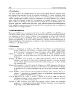
Figure 7a shows the trends of steady-state flow rate versus needle lift at rail pressures of 10
and 20 MPa, while the back pressure in the Bosch measuring tube was kept to either ambient
pressure or 4 MPa; whereas Figure 7b shows the resulting stationary hole discharge coefficient,
evaluated for the nozzle under investigation.
Taking advantage of the reduced variation of µ
s
h
with operation pressure, it is possible to
use the measured values to extrapolate the trends of steady-state discharge coefficient for
higher pressures, thus defining the upper boundary of variation of the nozzle hole discharge
coefficient values.
During the injector opening phase the unsteady effects are predominant and the sinusoidal-
linear trend of the hole discharge coefficient, Equation 10, was considered; when the needle-
seat relative displacement approaches its relative maximum value ξ
r
M
, the discharge coeffi-
cient increases in time, which means that the efflux through the nozzle holes is moving to
the stationary conditions. In order to describe this behavior, a transition phase between the
Accurate modelling of an injector for common rail systems 103
2.1.3 Discharge coefficient of the nozzle holes
The model of the discharge coefficient of the nozzle holes is designed on the base of the un-
steady coefficients reported in (Catania et al., 1994; 1997). These coefficients were experimen-
tally evaluated for minisac and VCO nozzles in the real working conditions of a distributor
pump-valve-pipe-injector type injection system. The pattern of this coefficient versus needle
lift evidences three different phases. In the first phase, during injector opening, the moving

needle tip strongly influences the efflux through the nozzle holes. In this phase, the discharge
coefficient progressively increases with the needle lift. In the second phase, when the needle
is at its maximum stroke, the discharge coefficient increases in time, independently from the
pressure level at the injector inlet. In the last phase, during the needle closing stroke, the dis-
charge coefficient remains almost constant. These three phases above mentioned describe a
hysteresis-like phenomenon. In order to build a model suitable for a common rail injector in
its whole operation field these three phases need to be considered.
Therefore, the nozzle hole discharge coefficient is modeled as needle lift dependent by con-
sidering two limit curves: a lower limit trend (µ
d
h
), which models the discharge coefficient in
transient efflux conditions, and an upper limit trend (µ
s
h
), which represents the steady-state
value of the discharge coefficient for a given needle lift. The evolution from transient to sta-
tionary values is modeled with a first order system dynamics.
It was experimentally observed (Catania et al., 1994; 1997) that the transient trend presents a
first region in which the discharge coefficient increases rapidly with needle lift, following a
sinusoidal-like pattern, and a second region, characterized by a linear dependence between
discharge coefficient and needle lift. Thus, the following model is adopted:
µ
d
h
(ξ) =

µ
d
h

(ξ
0
) sin(
π
2ξ
0
ξ) 0 ≤ ξ < ξ
0
µ
d
h
(ξ
M
)−µ
d
h
(ξ
0
)
ξ
M
−ξ
0
(ξ − ξ
0
) + µ
d
h
(ξ
0

) ξ ≥ ξ
0
(10)
where ξ is the needle-seat relative displacement, and ξ
0
is the transition value of ξ between
the sinusoidal and the linear trend.
The use of the variable ξ, rather than the needle lift, x
n
, emphasizes the fact that all the me-
chanical elements subject to fuel pressure, including nozzle and needle, deform, thus the real
variable controlling the discharge coefficient is not the position of the needle, but rather the
effective clearance between the latter and the nozzle.
The maximum needle lift, ξ
M
, varies with rail pressure due to the different level of deforma-
tion that this parameter induces on the mechanical components of the injector. The relation
between ξ
M
and the reference rail pressure p
r0
is assumed to be linear as
ξ
M
= K
1
p
r0
+ K
2

(11)
where K
1
and K
2
are constants that are evaluated as explained in the section 2.3.3.
Similarly, the value of ξ
0
in Equation 10 is modeled as a function of the operating pressure p
r0
in order to better match the experimental behavior of the injection system. Thus, the following
fit is used
ξ
0
= K
3
p
r0
+ K
4
(12)
and K
3
and K
4
are obtained at the end of the model tuning phase (table 4).
In order to define the relation between the steady state value of the nozzle-hole discharge
coefficient (µ
s
h

) and the needle-seat relative displacement (ξ) the device in Figure 6 was de-
signed. It contains a camshaft that can impose to the needle a continuously variable lift up to
1 mm. Then, a modified injector equipped with this device was connected to the common rail
injection system and installed in a Bosch measuring tube, in order to control the nozzle hole
downstream pressure. The steady flow rate was measured by means of a set of graduated
burettes.
1. Dial indicator 4. Eccentric ball bearing (e = 1mm)
2. Handing for varying needle lift 5. Injector control piston
3. Axis support bearing 6. Injector inlet
Fig. 6. Device for fixed needle-seat displacement imposition
Figure 7a shows the trends of steady-state flow rate versus needle lift at rail pressures of 10
and 20 MPa, while the back pressure in the Bosch measuring tube was kept to either ambient
pressure or 4 MPa; whereas Figure 7b shows the resulting stationary hole discharge coefficient,
evaluated for the nozzle under investigation.
Taking advantage of the reduced variation of µ
s
h
with operation pressure, it is possible to
use the measured values to extrapolate the trends of steady-state discharge coefficient for
higher pressures, thus defining the upper boundary of variation of the nozzle hole discharge
coefficient values.
During the injector opening phase the unsteady effects are predominant and the sinusoidal-
linear trend of the hole discharge coefficient, Equation 10, was considered; when the needle-
seat relative displacement approaches its relative maximum value ξ
r
M
, the discharge coeffi-
cient increases in time, which means that the efflux through the nozzle holes is moving to
the stationary conditions. In order to describe this behavior, a transition phase between the
Fuel Injection104

(a) Steady flow rate (b) Stationary discharge coefficient
Fig. 7. Stationary efflux through the nozzle
unsteady and the stationary values of the hole discharge coefficient at this needle lift was
considered. This phase was modeled as a temporal exponential curve, namely,
µ
h
= µ
d
h
(ξ
r
M
) + [µ
s
h
(ξ
r
M
) − µ
d
h
(ξ
r
M
)] [1 − exp (−
t − t
0
τ
)] (13)
where t

0
is the instant in time at which the needle-seat relative displacement approaches its
maximum value ξ
r
M
, µ
d
h

ξ
r
M

and µ
s
h

ξ
r
M

are the unsteady and the stationary hole discharge
coefficients evaluated at this needle-seat relative displacement, and τ is the time constant of
this phenomenon, which have to be defined during the model tuning phase.
Figure 8 shows the computed nozzle hole discharge coefficient, µ
h
, dependence upon needle-
seat relative displacement, ξ, in accordance to the proposed model, in a wide range of op-
erating conditions (which are showed by rail pressure p
r0

and energisation time ET
0
in the
legend).
Examining the discharge coefficient, µ
h
, trends for the three main injections (ET
0
= 780 µs, 700
µs and 670 µs) during the opening phase, it is interesting to note that for a given value of the
needle lift, lower discharge coefficients are to be expected at higher operating pressures. This
can be explained considering that the flow takes longer to develop if the pressure differential,
and thus the steady state velocity to reach is higher.
The main injection trends also show the transition from the sinusoidal to the linear depen-
dence of the transient discharge coefficient on needle lift.
The phase in which the needle has reached the maximum value and the discharge coefficient
increases in time from unsteady to stationary values is not very evident in main injections,
because the former increases enough during the opening phase to approach the latter. This
happens because the needle reaches sufficiently high lifts as to have reduced effect on the flow
in the nozzle holes, and the longer injection allows time for complete flow development.
Conversely, during pilot injections (ET
0
=300 µs), the needle reaches lower maximum lifts,
hence lower values of the unsteady discharge coefficient, so that the phase of transition to
the stationary value lasts longer. The beginning of this transition can be easily identified by
analyzing the curves marked with dots and crosses in Figure 8. The point at which they
depart from their main injection counterpart (same line style but without markers) marks the
beginning of the exponential evolution in time to stationary value of discharge coefficient.
For both pilot and main injections, the nozzle hole discharge coefficient remains constant, and
equal to the stationary value, during the injector closing phase, as shown by the horizontal

profile of the trends in Figure 8.
The needle-seat discharge coefficient µ
s
has to be modeled too. It is assumed as needle lift
dependent according to (Xu et al., 1992) where this coefficient was experimentally evaluated
after removing the nozzle tip. A three segment trend is considered, as shown in Fig. 8, but it
is worth to point out that it plays a marginal role in the injection system simulation because
its values are higher than 0.8 for most needle lift values.
Fig. 8. Needle-seat and holes discharge coefficient
2.1.4 One-dimensional model: pipe flow model
A one-dimensional modelling approach is followed in order to model the fluid flow in the
pipe connecting injector and rail and in the injector internal duct that carries the fluid from
the inlet to the delivery chamber. This is necessary to correctly take into account pressure
wave propagation that occurs in those elements. The pipe flow conservation equations are
written for a single-phase fluid because in the common-rail injection system cavitation does
not appear in the connecting pipe. An isothermal flow is assumed and only the momentum
and mass conservation equations need to be solved
∂w
∂t
+ A
∂w
∂x
= b (14)
where w
=

u
p

, A

=

u 1/ρ
ρc
2
u

, b
=

−4τ/ρd
0

and τ is the wall shear stress that is evaluated under the assumption of steady-state friction
(Streeter et al., 1998).
The eigenvalues of the hyperbolic system of partial differential Equations 14 are λ
= u ± c,
real and distinct. The celerity c of the wave propagation can be evaluated as
c
=




c
l

1
+ K
p

E
l
E
p
d
p
t
p

(15)
Accurate modelling of an injector for common rail systems 105
(a) Steady flow rate (b) Stationary discharge coefficient
Fig. 7. Stationary efflux through the nozzle
unsteady and the stationary values of the hole discharge coefficient at this needle lift was
considered. This phase was modeled as a temporal exponential curve, namely,
µ
h
= µ
d
h
(ξ
r
M
) + [µ
s
h
(ξ
r
M
) − µ

d
h
(ξ
r
M
)] [1 − exp (−
t − t
0
τ
)] (13)
where t
0
is the instant in time at which the needle-seat relative displacement approaches its
maximum value ξ
r
M
, µ
d
h

ξ
r
M

and µ
s
h

ξ
r

M

are the unsteady and the stationary hole discharge
coefficients evaluated at this needle-seat relative displacement, and τ is the time constant of
this phenomenon, which have to be defined during the model tuning phase.
Figure 8 shows the computed nozzle hole discharge coefficient, µ
h
, dependence upon needle-
seat relative displacement, ξ, in accordance to the proposed model, in a wide range of op-
erating conditions (which are showed by rail pressure p
r0
and energisation time ET
0
in the
legend).
Examining the discharge coefficient, µ
h
, trends for the three main injections (ET
0
= 780 µs, 700
µs and 670 µs) during the opening phase, it is interesting to note that for a given value of the
needle lift, lower discharge coefficients are to be expected at higher operating pressures. This
can be explained considering that the flow takes longer to develop if the pressure differential,
and thus the steady state velocity to reach is higher.
The main injection trends also show the transition from the sinusoidal to the linear depen-
dence of the transient discharge coefficient on needle lift.
The phase in which the needle has reached the maximum value and the discharge coefficient
increases in time from unsteady to stationary values is not very evident in main injections,
because the former increases enough during the opening phase to approach the latter. This
happens because the needle reaches sufficiently high lifts as to have reduced effect on the flow

in the nozzle holes, and the longer injection allows time for complete flow development.
Conversely, during pilot injections (ET
0
=300 µs), the needle reaches lower maximum lifts,
hence lower values of the unsteady discharge coefficient, so that the phase of transition to
the stationary value lasts longer. The beginning of this transition can be easily identified by
analyzing the curves marked with dots and crosses in Figure 8. The point at which they
depart from their main injection counterpart (same line style but without markers) marks the
beginning of the exponential evolution in time to stationary value of discharge coefficient.
For both pilot and main injections, the nozzle hole discharge coefficient remains constant, and
equal to the stationary value, during the injector closing phase, as shown by the horizontal
profile of the trends in Figure 8.
The needle-seat discharge coefficient µ
s
has to be modeled too. It is assumed as needle lift
dependent according to (Xu et al., 1992) where this coefficient was experimentally evaluated
after removing the nozzle tip. A three segment trend is considered, as shown in Fig. 8, but it
is worth to point out that it plays a marginal role in the injection system simulation because
its values are higher than 0.8 for most needle lift values.
Fig. 8. Needle-seat and holes discharge coefficient
2.1.4 One-dimensional model: pipe flow model
A one-dimensional modelling approach is followed in order to model the fluid flow in the
pipe connecting injector and rail and in the injector internal duct that carries the fluid from
the inlet to the delivery chamber. This is necessary to correctly take into account pressure
wave propagation that occurs in those elements. The pipe flow conservation equations are
written for a single-phase fluid because in the common-rail injection system cavitation does
not appear in the connecting pipe. An isothermal flow is assumed and only the momentum
and mass conservation equations need to be solved
∂w
∂t

+ A
∂w
∂x
= b (14)
where w
=

u
p

, A
=

u 1/ρ
ρc
2
u

, b
=

−4τ/ρd
0

and τ is the wall shear stress that is evaluated under the assumption of steady-state friction
(Streeter et al., 1998).
The eigenvalues of the hyperbolic system of partial differential Equations 14 are λ
= u ± c,
real and distinct. The celerity c of the wave propagation can be evaluated as
c

=




c
l

1
+ K
p
E
l
E
p
d
p
t
p

(15)
Fuel Injection106
where the second term within brackets takes into account the effect of the pipe elasticity; K
p
is the pipe constraint factor, depending on pipe support layout, E
p
the Young’s modulus of
elasticity of the pipe material, d
p
the pipe diameter and t

p
the pipe wall thickness (Streeter
et al., 1998). Being the pipe ends rigidly constrained, the pipe constrain factor K
p
can be
evaluated as
K
p
= 1 − ν
2
p
(16)
where ν
p
is the Poisson’s modulus of the pipe material.
Pipe junctions are treated as minor losses and only the continuity equation is locally written.
As mentioned before, this simple pipe flow model is not suitable when cavitation occurs.
This is not a limitation when common-rail injection system are modelled because of the high
pressure level at which these systems always work. In order to model conventional injection
systems, as pump-pipe-nozzle systems, it is necessary to employ a pipe flow model able to
simulate the cavitation occurrence. For this purpose the authors developed an appropriate
second order model (Dongiovanni et al., 2003).
2.1.5 Fluid properties
Thermodynamic properties of oil are affected by temperature and pressure that remarkably
vary in the common rail injection system operation field. Density, wave propagation speed
and kinematic viscosity of the ISO4113 air-free test oil had been evaluated as function of pres-
sure and temperature (Dongiovanni, 1997). These oil properties were approximated with an-
alytic functions of the exponential type in the range of pressures from 0.1 to 200 MPa and
temperatures from 10
◦

C to 120
◦
C. These analytic relations were derived from the actual
property values supplied by the oil maker, by using the least-square method for non-linear
approximation functions with two independent variables. The adopted formulae are:
ρ
l
(p, T) = K
ρ1
+

1
− exp

−
p
K
ρ2

K
ρ3
p
K
ρ4
(17)
E
l
(p, T) = K
E1
+


1
− exp

−
p
K
E2

K
E3
p
K
E4
(18)
ν
l
(p, T) = K
ν1
+ K
ν2
p
K
ν3
(19)
The K
Ei
, K
ρi
and K

νi
are polynomial functions of temperature T
K
i
=
l
i
∑
j=0
K
i,j
T
j
i = 1, 2, 3, 4 (20)
and the numerical coefficients that appear in them are reported in Table 2 according with
SI units: pressure
[p] = bar, temperature [T] =
◦
C, density [ρ
l
] = kg/m
3
, bulk modulus
[E
l
] = MPa and kinematic viscosity [ν
l
] = mm
2
/s

Finally, the celerity of the air free oil is evaluate in accordance with c
l
=

E
l
/ρ
l
.
By using these approximation functions, the maximum deviation between experimental and
analytical values in the examined range of pressure and temperature has been estimated as
being lower than
±0.2% for density, ±1.2% for bulk modulus, ±0.6% for celerity and ±18%
for kinematic viscosity.
K
ρ
j= 0 j= 1 j= 2
K
ρ1,j
8.3636e2 -6.7753e-1 -
K
ρ2,j
1.5063e2 -2.4202e-1 -
K
ρ3,j
1.7784e-1 1.4640e-3 1.5402e-5
K
ρ4,j
7.8109e-1 -8.1893e-4 -
K

E
j= 0 j= 1 j= 2
K
E1,j
1.7356e3 -1.0908e1 2.2976e-2
K
E2,j
7.5540e1 - -
K
E3,j
1.5050 -3.7603e-3 -
K
E4,j
9.4448e-1 3.9441e-4 -
K
ν
j=0 j=1 j=2 j=3
K
ν1,j
6.4862 -1.5847e-1 1.6342e-3 -6.0334e-6
K
ν2,j
4.0435e-4 -2.3118e-6 - -
K
ν3,j
1.4346 -6.2288e-3 3.3500e-5 -
Table 2. Polynomial coefficients for ISO4113 oil
2.2 Electromagnetic model
A model of the electromechanical actuator that drives the control valve must be realized in
order to work out the net mechanical force applied by the solenoid on its armature, for a given

current flowing in the solenoid. The magnetic force applied by the solenoid on the armature
F
Ea
can be obtained by applying the principle of energy conservation to the armature-coil
system (Chai, 1998; Nasar, 1995). In the general form it can be written as follows:
V I dt
= F
Ea
dx
a
+ dW
m
(21)
where V I dt represents the electric energy input to the system, F
Ea
dx
a
is the mechanical work
done on the armature and dW
m
is the change in the magnetic energy.
From Faraday’s law, voltage V may be expressed in terms of flux linkage (N
dΦ
dt
) and Equation
21 becomes
N I dΦ
= F
Ea
dx

a
+ dW
m
(22)
as shown in (Chai, 1998; Nasar, 1995); by considering Φ and x
a
as independent variables,
Equation 22 can be reduced to
F
Ea
= −
∂W
m
∂x
a




Φ
(23)
The magnetic circuit geometry of the control valve needs to be thoroughly analyzed in order
to evaluate the magnetic energy stored in the gap. Fig. 9a shows the path of the significant
magnetic fluxes, having neglected secondary leakage fluxes and flux fringing.
Exploiting the analogy between Ohm’s and Hopkinson’s law, it is possible to obtain the mag-
netic equivalent circuit of Fig. 9b where NI is the ampere-turns in the exciting coil and

j
(j = 1, , 5) are the magnetic reluctances. When the magnetic flux flows across a cross-
section area A

a
constant along the path length l, the value of the j-th reluctance can be ob-
tained by:
Accurate modelling of an injector for common rail systems 107
where the second term within brackets takes into account the effect of the pipe elasticity; K
p
is the pipe constraint factor, depending on pipe support layout, E
p
the Young’s modulus of
elasticity of the pipe material, d
p
the pipe diameter and t
p
the pipe wall thickness (Streeter
et al., 1998). Being the pipe ends rigidly constrained, the pipe constrain factor K
p
can be
evaluated as
K
p
= 1 − ν
2
p
(16)
where ν
p
is the Poisson’s modulus of the pipe material.
Pipe junctions are treated as minor losses and only the continuity equation is locally written.
As mentioned before, this simple pipe flow model is not suitable when cavitation occurs.
This is not a limitation when common-rail injection system are modelled because of the high

pressure level at which these systems always work. In order to model conventional injection
systems, as pump-pipe-nozzle systems, it is necessary to employ a pipe flow model able to
simulate the cavitation occurrence. For this purpose the authors developed an appropriate
second order model (Dongiovanni et al., 2003).
2.1.5 Fluid properties
Thermodynamic properties of oil are affected by temperature and pressure that remarkably
vary in the common rail injection system operation field. Density, wave propagation speed
and kinematic viscosity of the ISO4113 air-free test oil had been evaluated as function of pres-
sure and temperature (Dongiovanni, 1997). These oil properties were approximated with an-
alytic functions of the exponential type in the range of pressures from 0.1 to 200 MPa and
temperatures from 10
◦
C to 120
◦
C. These analytic relations were derived from the actual
property values supplied by the oil maker, by using the least-square method for non-linear
approximation functions with two independent variables. The adopted formulae are:
ρ
l
(p, T) = K
ρ1
+

1
− exp

−
p
K
ρ2


K
ρ3
p
K
ρ4
(17)
E
l
(p, T) = K
E1
+

1
− exp

−
p
K
E2

K
E3
p
K
E4
(18)
ν
l
(p, T) = K

ν1
+ K
ν2
p
K
ν3
(19)
The K
Ei
, K
ρi
and K
νi
are polynomial functions of temperature T
K
i
=
l
i
∑
j=0
K
i,j
T
j
i = 1, 2, 3, 4 (20)
and the numerical coefficients that appear in them are reported in Table 2 according with
SI units: pressure
[p] = bar, temperature [T] =
◦

C, density [ρ
l
] = kg/m
3
, bulk modulus
[E
l
] = MPa and kinematic viscosity [ν
l
] = mm
2
/s
Finally, the celerity of the air free oil is evaluate in accordance with c
l
=

E
l
/ρ
l
.
By using these approximation functions, the maximum deviation between experimental and
analytical values in the examined range of pressure and temperature has been estimated as
being lower than
±0.2% for density, ±1.2% for bulk modulus, ±0.6% for celerity and ±18%
for kinematic viscosity.
K
ρ
j= 0 j= 1 j= 2
K

ρ1,j
8.3636e2 -6.7753e-1 -
K
ρ2,j
1.5063e2 -2.4202e-1 -
K
ρ3,j
1.7784e-1 1.4640e-3 1.5402e-5
K
ρ4,j
7.8109e-1 -8.1893e-4 -
K
E
j= 0 j= 1 j= 2
K
E1,j
1.7356e3 -1.0908e1 2.2976e-2
K
E2,j
7.5540e1 - -
K
E3,j
1.5050 -3.7603e-3 -
K
E4,j
9.4448e-1 3.9441e-4 -
K
ν
j=0 j=1 j=2 j=3
K

ν1,j
6.4862 -1.5847e-1 1.6342e-3 -6.0334e-6
K
ν2,j
4.0435e-4 -2.3118e-6 - -
K
ν3,j
1.4346 -6.2288e-3 3.3500e-5 -
Table 2. Polynomial coefficients for ISO4113 oil
2.2 Electromagnetic model
A model of the electromechanical actuator that drives the control valve must be realized in
order to work out the net mechanical force applied by the solenoid on its armature, for a given
current flowing in the solenoid. The magnetic force applied by the solenoid on the armature
F
Ea
can be obtained by applying the principle of energy conservation to the armature-coil
system (Chai, 1998; Nasar, 1995). In the general form it can be written as follows:
V I dt
= F
Ea
dx
a
+ dW
m
(21)
where V I dt represents the electric energy input to the system, F
Ea
dx
a
is the mechanical work

done on the armature and dW
m
is the change in the magnetic energy.
From Faraday’s law, voltage V may be expressed in terms of flux linkage (N
dΦ
dt
) and Equation
21 becomes
N I dΦ
= F
Ea
dx
a
+ dW
m
(22)
as shown in (Chai, 1998; Nasar, 1995); by considering Φ and x
a
as independent variables,
Equation 22 can be reduced to
F
Ea
= −
∂W
m
∂x
a





Φ
(23)
The magnetic circuit geometry of the control valve needs to be thoroughly analyzed in order
to evaluate the magnetic energy stored in the gap. Fig. 9a shows the path of the significant
magnetic fluxes, having neglected secondary leakage fluxes and flux fringing.
Exploiting the analogy between Ohm’s and Hopkinson’s law, it is possible to obtain the mag-
netic equivalent circuit of Fig. 9b where NI is the ampere-turns in the exciting coil and

j
(j = 1, , 5) are the magnetic reluctances. When the magnetic flux flows across a cross-
section area A
a
constant along the path length l, the value of the j-th reluctance can be ob-
tained by:
Fuel Injection108
(a) Magnetic path (b) Magnetic equivalent circuit
Fig. 9. Magnetic model sketch

j
=
l
j
µ
0
A
aj
(j = 1, 2) (24)
When the flux flows across a radial path, the reluctance can be evaluated as


j
=
1
2πµ
0
t
j
ln

d
e
d
i

j
(j = 3, 4, 5) (25)
being t the radial thickness, d
e
and d
i
the external and internal diameter of the gap volume.
Reluctance of the ferromagnetic components was neglected because it is several order of mag-
nitude lower than the corresponding gap reluctance.
Circuit of Fig. 9b is solved using Thevenin’s theorem, and the equivalent circuit reluctance
connected to the magnetomotive force generator is determined as
 = 
1
+

2


3

4
+ 
2

5
(

3
+ 
4
)

3

4
+
(

2
+ 
5
) (

3
+ 
4
)

(26)
The magnetic energy W
m
is stored in the volume of the electromechanical actuator, but only
the portion of energy stored in the gap between control-valve body and magnetic core de-
pends on the armature lift x
a
. Consequently, being the magnetization curve of non-ferromagnetic
materials (oil in the gaps) linear, Equation 23 can be written as
F
Ea
= −
1
2
Φ
2
d
dx
a
= −
1
2

NI


2
d
dx
a

(27)
To complete the model, it was necessary to take into account the saturation phenomenon that
occurs to every ferromagnetic material. That is, a magnetic flux cannot increase indefinitely, as
the material presents a maximum magnetic flux density after which the curve B
− H is almost
flat. In this model we assumed a simplified magnetization curve, given by :
B
=

µH H
< H
∗
µH
∗
+ µ
0
(
H − H
∗
)
H ≥ H
∗
(28)
thus neglecting material hysteresis and non-linearity.
As a result of the saturation phenomenon, the maximum force of attraction is limited because
the maximum magnetic flux which can be obtained in the j-th branch of the circuit is approx-
imately
Φ
Mj
≈ µH

∗
j
A
j
(29)
being µ
0
negligible with respect µ.
The most important parameters in the electromagnetic model are set as reported in Table 3.
N B
∗
= µH
∗
[T] t
3
[mm] t
4
[mm] t
5
[mm]
32 2.5 0.65 1.5 0.05
Table 3. Most important electromagnetic model parameters
The model was employed to evaluate the inductance of the solenoid when mounted on the
injector body. In this case, with the valve actuator in the closed position, an inductance of 134
µH was evaluated. Employing a sinusoidal wave generator at a frequency of 5 kHz, which
is high enough to make negligible the mechanical system movements, an inductance of 137
µH was measured. The accordance between experimental and theoretical inductance value
indirectly validates the electromagnetic model and the parameters value.
Fig. 10a shows the theoretical (solid line) driving actuator force when the actual energizing
current (dashed line) is used to feeding the injector solenoid.

(a) Magnetic force and feeding current (b) Inductance and armature lift
Fig. 10. Magnetic model results
Furthermore, we point out that the measure of the injector coil inductance L
= N/
2
could
be used to indirectly evaluate the control valve lift, due to the dependence of reluctance upon
armature distance from the solenoid (Equation 24 ).
Bearing in mind that, by applying Ohm’s law to the solenoid coil, the inductance L could be
evaluated as:
L
=

(
V − RI
)
dt
I
(30)
hence only the measurement of solenoid current I and voltage V would be required to calcu-
late L.
Accurate modelling of an injector for common rail systems 109
(a) Magnetic path (b) Magnetic equivalent circuit
Fig. 9. Magnetic model sketch

j
=
l
j
µ

0
A
aj
(j = 1, 2) (24)
When the flux flows across a radial path, the reluctance can be evaluated as

j
=
1
2πµ
0
t
j
ln

d
e
d
i

j
(j = 3, 4, 5) (25)
being t the radial thickness, d
e
and d
i
the external and internal diameter of the gap volume.
Reluctance of the ferromagnetic components was neglected because it is several order of mag-
nitude lower than the corresponding gap reluctance.
Circuit of Fig. 9b is solved using Thevenin’s theorem, and the equivalent circuit reluctance

connected to the magnetomotive force generator is determined as
 = 
1
+

2

3

4
+ 
2

5
(

3
+ 
4
)

3

4
+
(

2
+ 
5

) (

3
+ 
4
)
(26)
The magnetic energy W
m
is stored in the volume of the electromechanical actuator, but only
the portion of energy stored in the gap between control-valve body and magnetic core de-
pends on the armature lift x
a
. Consequently, being the magnetization curve of non-ferromagnetic
materials (oil in the gaps) linear, Equation 23 can be written as
F
Ea
= −
1
2
Φ
2
d
dx
a
= −
1
2

NI



2
d
dx
a
(27)
To complete the model, it was necessary to take into account the saturation phenomenon that
occurs to every ferromagnetic material. That is, a magnetic flux cannot increase indefinitely, as
the material presents a maximum magnetic flux density after which the curve B
− H is almost
flat. In this model we assumed a simplified magnetization curve, given by :
B
=

µH H
< H
∗
µH
∗
+ µ
0
(
H − H
∗
)
H ≥ H
∗
(28)
thus neglecting material hysteresis and non-linearity.

As a result of the saturation phenomenon, the maximum force of attraction is limited because
the maximum magnetic flux which can be obtained in the j-th branch of the circuit is approx-
imately
Φ
Mj
≈ µH
∗
j
A
j
(29)
being µ
0
negligible with respect µ.
The most important parameters in the electromagnetic model are set as reported in Table 3.
N B
∗
= µH
∗
[T] t
3
[mm] t
4
[mm] t
5
[mm]
32 2.5 0.65 1.5 0.05
Table 3. Most important electromagnetic model parameters
The model was employed to evaluate the inductance of the solenoid when mounted on the
injector body. In this case, with the valve actuator in the closed position, an inductance of 134

µH was evaluated. Employing a sinusoidal wave generator at a frequency of 5 kHz, which
is high enough to make negligible the mechanical system movements, an inductance of 137
µH was measured. The accordance between experimental and theoretical inductance value
indirectly validates the electromagnetic model and the parameters value.
Fig. 10a shows the theoretical (solid line) driving actuator force when the actual energizing
current (dashed line) is used to feeding the injector solenoid.
(a) Magnetic force and feeding current (b) Inductance and armature lift
Fig. 10. Magnetic model results
Furthermore, we point out that the measure of the injector coil inductance L
= N/
2
could
be used to indirectly evaluate the control valve lift, due to the dependence of reluctance upon
armature distance from the solenoid (Equation 24 ).
Bearing in mind that, by applying Ohm’s law to the solenoid coil, the inductance L could be
evaluated as:
L
=

(
V − RI
)
dt
I
(30)
hence only the measurement of solenoid current I and voltage V would be required to calcu-
late L.
Fuel Injection110
Fig. 10b draws the theoretical inductance L, which was calculated according to Equation 24
and opportunely scaled, compared to the experimental valve lift x

c
, showing a good agree-
ment between the two trends, and hence the potential of this non-invasive measurement tech-
nique. However, Equation 30 is only applicable when electric current is flowing in the solenoid
coil so, for example, it is not possible to use this method to record the the control valve closure
trend because, as Fig. 10b shows, this usually begins when the solenoid current is null.
A possible way to solve this problem would be to inject an additional, small amplitude, high
frequency (around 1 MHz) current into the coil, but this technique has not yet been tested by
the authors.
2.3 Mechanical model
All mechanical devices that can move during injector functioning (i.e. needle, control piston
and control valve) are modelled using the conventional mass-spring-damper scheme, gov-
erned by a mechanical equilibrium equation, in which the dynamic parameters are function
of element position.
m
j
d
2
x
j
dt
2
+ β
j
dx
j
dt
+ k
j
x

j
+ F
0j
= F
j
(31)
where m
j
is the displacing mass, β
j
the damping coefficient, k
j
the spring stiffness and F
0
j
the spring preload; the bar above the symbols indicates that these coefficients are evaluated
according to the relative position of the moving elements.
2.3.1 Control piston, needle and nozzle model
The high working pressures in the common-rail injection system stress its components and
cause appreciable deformation of them. In order to take into account the effects of the axial
deformation of nozzle and injector body, the nozzle is modelled by means of a conventional
mass-spring-damper scheme as well as the needle and the control piston, while the injector
body is modelled by means of a simple spring having appropriate stiffness.
Injector needle, control piston and nozzle form a three degrees of freedom mechanical system,
which can be modelled as shown in Figure 11a. Three equilibrium equations are needed to
describe the system motion, one for each element. With reference to Fig. 11a, the dynamic
equilibrium Equation 31 is written using the following definition for the control piston (j
= P),
the needle (j
= n) and the nozzle (j = N):

external force F
j
:
F
P
= −F
c
+ p
T
S
P
+ F
R(Pn)
− F
R(Pb)
F
n
= −p
T
S
n
− F
R(Pn)
+ F
S
+ F
R(nN)
F
N
= −F

S
+ p
e
S
n
− F
R(nN)
(32)
where F
R(ij)
is the force that i-th and j-th element apply to each other when they are in contact,
F
c
= p
uA
S

P
+ p
dZ
(S
P
− S

P
) (33)
and
F
S
= p

S
S
S
+ p
D
S
D
+ [γ p
S
+ (1 − γ) p
D
)] (S
n
− S
D
− S
S
) (34)
where γ
= 0 indicates that the nozzle is closed while γ = 1 indicates open nozzle conditions.
Damping coefficient
β
j
, stiffness k
j
and preload F
0j
are evaluated as follows for:
control piston
(a) Control piston and needle (b) Control valve

Fig. 11. Dynamic models
x
P
< X
MP
− l
P
β
P
= β
P
k
P
= 0 F
0P
= 0
X
MP
− l
P
≤ x
P
β
P
= β
b
+ β
P
k
P

= k
b
F
0P
= −k
b
(X
MP
− l
P
)
(35)
needle
x
n
− x
N
< 0 β
n
= β
b
+ β
n
k
n
= k
b
+ k
n
F

0n
= F
0n
0 ≤ x
n
− x
N
< X
Mn
− l
n
β
n
= β
n
k
n
= k
n
F
0n
= F
0n
X
Mn
− l
n
≤ x
n
− x

N
β
n
= β
b
+ β
n
k
n
= k
b
+ k
n
F
0n
= F
0n
− k
b
X
Mn
(36)
nozzle
x
n
− x
N
< 0 β
N
= β

b
+ β
N
k
N
= k
b
+ k
N
F
0N
= 0
0
≤ x
n
− x
N
β
N
= β
N
k
N
= k
N
F
0N
= 0
(37)
2.3.2 Control valve model

The control valve contains two mobile parts: the pin element having mass m
c
and the armature
element of mass m
a
; they can be modelled with the two degrees of freedom scheme shown in
Fig. 11b. The two dynamic equilibrium equations are written in a similar fashion as Equation
31 where j
= a indicates the armature and j = c the control-pin. The external forces F
j
can be
evaluated as
F
a
= F
Ea
− F
R(ca)
F
c
= (p
dA
− p
T
)S
c
+ F
R(ca)
+ F
R(c b)

(38)
where F
Ea
represents the electromagnetic action that the current generates when it flows in
the solenoid coil determined as shown in section 2.2.
Accurate modelling of an injector for common rail systems 111
Fig. 10b draws the theoretical inductance L, which was calculated according to Equation 24
and opportunely scaled, compared to the experimental valve lift x
c
, showing a good agree-
ment between the two trends, and hence the potential of this non-invasive measurement tech-
nique. However, Equation 30 is only applicable when electric current is flowing in the solenoid
coil so, for example, it is not possible to use this method to record the the control valve closure
trend because, as Fig. 10b shows, this usually begins when the solenoid current is null.
A possible way to solve this problem would be to inject an additional, small amplitude, high
frequency (around 1 MHz) current into the coil, but this technique has not yet been tested by
the authors.
2.3 Mechanical model
All mechanical devices that can move during injector functioning (i.e. needle, control piston
and control valve) are modelled using the conventional mass-spring-damper scheme, gov-
erned by a mechanical equilibrium equation, in which the dynamic parameters are function
of element position.
m
j
d
2
x
j
dt
2

+ β
j
dx
j
dt
+ k
j
x
j
+ F
0j
= F
j
(31)
where m
j
is the displacing mass, β
j
the damping coefficient, k
j
the spring stiffness and F
0
j
the spring preload; the bar above the symbols indicates that these coefficients are evaluated
according to the relative position of the moving elements.
2.3.1 Control piston, needle and nozzle model
The high working pressures in the common-rail injection system stress its components and
cause appreciable deformation of them. In order to take into account the effects of the axial
deformation of nozzle and injector body, the nozzle is modelled by means of a conventional
mass-spring-damper scheme as well as the needle and the control piston, while the injector

body is modelled by means of a simple spring having appropriate stiffness.
Injector needle, control piston and nozzle form a three degrees of freedom mechanical system,
which can be modelled as shown in Figure 11a. Three equilibrium equations are needed to
describe the system motion, one for each element. With reference to Fig. 11a, the dynamic
equilibrium Equation 31 is written using the following definition for the control piston (j
= P),
the needle (j
= n) and the nozzle (j = N):
external force F
j
:
F
P
= −F
c
+ p
T
S
P
+ F
R(Pn)
− F
R(Pb)
F
n
= −p
T
S
n
− F

R(Pn)
+ F
S
+ F
R(nN)
F
N
= −F
S
+ p
e
S
n
− F
R(nN)
(32)
where F
R(ij)
is the force that i-th and j-th element apply to each other when they are in contact,
F
c
= p
uA
S

P
+ p
dZ
(S
P

− S

P
) (33)
and
F
S
= p
S
S
S
+ p
D
S
D
+ [γ p
S
+ (1 − γ) p
D
)] (S
n
− S
D
− S
S
) (34)
where γ
= 0 indicates that the nozzle is closed while γ = 1 indicates open nozzle conditions.
Damping coefficient β
j

, stiffness k
j
and preload F
0j
are evaluated as follows for:
control piston
(a) Control piston and needle (b) Control valve
Fig. 11. Dynamic models
x
P
< X
MP
− l
P
β
P
= β
P
k
P
= 0 F
0P
= 0
X
MP
− l
P
≤ x
P
β

P
= β
b
+ β
P
k
P
= k
b
F
0P
= −k
b
(X
MP
− l
P
)
(35)
needle
x
n
− x
N
< 0 β
n
= β
b
+ β
n

k
n
= k
b
+ k
n
F
0n
= F
0n
0 ≤ x
n
− x
N
< X
Mn
− l
n
β
n
= β
n
k
n
= k
n
F
0n
= F
0n

X
Mn
− l
n
≤ x
n
− x
N
β
n
= β
b
+ β
n
k
n
= k
b
+ k
n
F
0n
= F
0n
− k
b
X
Mn
(36)
nozzle

x
n
− x
N
< 0 β
N
= β
b
+ β
N
k
N
= k
b
+ k
N
F
0N
= 0
0
≤ x
n
− x
N
β
N
= β
N
k
N

= k
N
F
0N
= 0
(37)
2.3.2 Control valve model
The control valve contains two mobile parts: the pin element having mass m
c
and the armature
element of mass m
a
; they can be modelled with the two degrees of freedom scheme shown in
Fig. 11b. The two dynamic equilibrium equations are written in a similar fashion as Equation
31 where j
= a indicates the armature and j = c the control-pin. The external forces F
j
can be
evaluated as
F
a
= F
Ea
− F
R(ca)
F
c
= (p
dA
− p

T
)S
c
+ F
R(ca)
+ F
R(c b)
(38)
where F
Ea
represents the electromagnetic action that the current generates when it flows in
the solenoid coil determined as shown in section 2.2.
Fuel Injection112
Damping coefficient β
j
, stiffness k
j
and preload F
0j
are evaluated as follows:
pin element
x
c
< 0 β
c
= β
b
+ β
c
k

c
= k
b
+ k
c
F
0c
= F
0c
0 ≤ x
c
< X
Mc
− l
c
β
c
= β
c
k
c
= k
c
F
0c
= F
0c
X
Mc
− l

c
≤ x
c
β
c
= β
b
+ β
c
k
c
= k
b
+ k
c
F
0c
= F
0c
− k
b
(X
Mc
− l
c
)
(39)
armature
l
Mc

− X
Mc
+ x
c
≥ x
a
β
a
= β
a
k
a
= k
a
F
0a
= F
0a
x
a
> l
Mc
− X
Mc
+ x
c
β
a
= β
b

+ β
a
k
a
= k
b
+ k
a
F
0a
= F
0a
− k
b
(l
Mc
− X
Mc
+ x
c
)
(40)
2.3.3 Mechanical components deformation
The axial deformation of needle, nozzle and control piston have to be taken into account.
These elements are considered only axially stressed, while the effects of the radial stress are
neglected. For the sake of simplicity, the axial length of control piston (l
P
), needle (l
n
), and

nozzle (l
N
) can be evaluated as function of the axial compressive load (F
C
) in each element.
Therefore, the deformed length l of these elements, which are considered formed by m parts
having cross section A
j
and initial length l
0
j
, is evaluated as follows
l
=
m
∑
j
l
0
j

1
−
F
C
j
EA
j

(41)

where E is Young’s modulus of the considered material.
The axial deformation of the injector body is taken into account by introducing in the model
the elastic elements indicated as k
B
and k
Bc
in Figure 11.
The injector body deformation cannot be theoretically calculated very easily, because one
should need to take into account the effect and the deformation of the constraints that fix
the injector on the test rig. For this reason, in order to evaluate the elasticity coefficient of k
B
and k
Bc
, an empirical approach is followed, which consists in obtaining a relation between
the axial length of these elements and the fluid pressure inside the injector body. As direct
consequence, the maximum stroke of the needle-control piston (ξ
M
) and of the control-valve
(X
Mc
) can be expressed as a function of the injector structural stress.
(a) Needle (b) Control valve
Fig. 12. Effect of pressure on the maximum moving element lift
Figure 12 reports the actual maximum needle-control piston lift (circular symbols) as a func-
tion of rail pressure. At the rail pressure of 30 MPa the maximum needle-control piston lift was
not reached, so no value is reported at this rail pressure. The continuous line represents the
least-square fit interpolating the experimental data and the dashed line shows the maximum
needle-control piston lift calculated by considering only nozzle, needle and control-piston ax-
ial deformation. The difference between the two lines represents the effect of the injector body
deformation on the maximum needle-control piston lift. This can be expressed as a function

of rail pressure and, for the considered injector, can be estimated in 0.41 µm/MPa. By means
of the linear fit (continuous line) reported in Figure 12 it is possible to evaluate the parameters
K
1
= 1.59 µm/MPa and K
2
= 364 µm that appear in Eq. 11.
In order to evaluate the elasticity coefficient k
Bc
, an analogous procedure can be followed
by analyzing the maximum control-valve lift dependence upon fuel pressure, as shown in
Figure 12. It was found that the effect of injector body deformation was that of reducing the
maximum control valve stroke of 0.06 µm/MPa.
(a) p
r0
=140 MPa, ET
0
= 1230 µs (b) p
r0
=80 MPa, ET
0
= 1230 µs
Fig. 13. Deformation effects on needle lift
The relevance of the deformation effects on the injector predicted performances is shown in
Fig. 13. The left graph shows the control piston lift at a rail pressure of 140 MPa generated with
an energizing time ET
0
of 1230µs, while the right graph shows the same trend at a rail pressure
of 80 MPa, and generated with the same value of ET
0

. The experimental results are drawn by
circular symbols, while lines refer to theoretical results. The dashed lines (Model a) show the
theoretical control piston lift evaluated by only taking in to account the axial deformation of
the moving elements and nozzle, while the continuous lines (Model b) show the theoretical
results evaluated by taking into account the injector body deformation too. The difference
between the two models is significant, and so is the underestimation of the volume of fluid
injected per stroke (4.3% with p
r0
=140MPa and ET
0
of 1230µs, 3.6% with p
r0
=80MPa, ET
0
of
1230µs). This highlights the necessity of accounting for deformation of the entire injector body,
if accurate predictions are sought.
Indeed, the maximum needle lift evaluation plays an important role in the simulation of the
injector behaviour in its whole operation field because it influences both the calculation of the
injected flow rate (as the discharge coefficients of needle-seat and nozzle holes depend also
on needle lift) and of the injector closing time, thus strongly affecting the predicted volume of
fuel injected per cycle.
The deformation of the injector body also affects the maximum control valve stroke, and a
similar analysis can be performed to evaluate its effects on injector performance. Our study
showed that this parameter does not play as important a role as the maximum needle stroke,
because the effective flow area of the A hole is smaller than the one generated by the displace-
ment of the control valve pin, and thus it is the A hole that controls the efflux from the control
volume to the tank.