Fuel Injection Part 7 pot
Bạn đang xem bản rút gọn của tài liệu. Xem và tải ngay bản đầy đủ của tài liệu tại đây (1.41 MB, 20 trang )
Accurate modelling of an injector for common rail systems 113
Damping coefficient β
j
, stiffness k
j
and preload F
0j
are evaluated as follows:
pin element
x
c
< 0 β
c
= β
b
+ β
c
k
c
= k
b
+ k
c
F
0c
= F
0c
0 ≤ x
c
< X
Mc
− l
c
β
c
= β
c
k
c
= k
c
F
0c
= F
0c
X
Mc
− l
c
≤ x
c
β
c
= β
b
+ β
c
k
c
= k
b
+ k
c
F
0c
= F
0c
− k
b
(X
Mc
− l
c
)
(39)
armature
l
Mc
− X
Mc
+ x
c
≥ x
a
β
a
= β
a
k
a
= k
a
F
0a
= F
0a
x
a
> l
Mc
− X
Mc
+ x
c
β
a
= β
b
+ β
a
k
a
= k
b
+ k
a
F
0a
= F
0a
− k
b
(l
Mc
− X
Mc
+ x
c
)
(40)
2.3.3 Mechanical components deformation
The axial deformation of needle, nozzle and control piston have to be taken into account.
These elements are considered only axially stressed, while the effects of the radial stress are
neglected. For the sake of simplicity, the axial length of control piston (l
P
), needle (l
n
), and
nozzle (l
N
) can be evaluated as function of the axial compressive load (F
C
) in each element.
Therefore, the deformed length l of these elements, which are considered formed by m parts
having cross section A
j
and initial length l
0
j
, is evaluated as follows
l
=
m
∑
j
l
0
j
1
−
F
C
j
EA
j
(41)
where E is Young’s modulus of the considered material.
The axial deformation of the injector body is taken into account by introducing in the model
the elastic elements indicated as k
B
and k
Bc
in Figure 11.
The injector body deformation cannot be theoretically calculated very easily, because one
should need to take into account the effect and the deformation of the constraints that fix
the injector on the test rig. For this reason, in order to evaluate the elasticity coefficient of k
B
and k
Bc
, an empirical approach is followed, which consists in obtaining a relation between
the axial length of these elements and the fluid pressure inside the injector body. As direct
consequence, the maximum stroke of the needle-control piston (ξ
M
) and of the control-valve
(X
Mc
) can be expressed as a function of the injector structural stress.
(a) Needle (b) Control valve
Fig. 12. Effect of pressure on the maximum moving element lift
Figure 12 reports the actual maximum needle-control piston lift (circular symbols) as a func-
tion of rail pressure. At the rail pressure of 30 MPa the maximum needle-control piston lift was
not reached, so no value is reported at this rail pressure. The continuous line represents the
least-square fit interpolating the experimental data and the dashed line shows the maximum
needle-control piston lift calculated by considering only nozzle, needle and control-piston ax-
ial deformation. The difference between the two lines represents the effect of the injector body
deformation on the maximum needle-control piston lift. This can be expressed as a function
of rail pressure and, for the considered injector, can be estimated in 0.41 µm/MPa. By means
of the linear fit (continuous line) reported in Figure 12 it is possible to evaluate the parameters
K
1
= 1.59 µm/MPa and K
2
= 364 µm that appear in Eq. 11.
In order to evaluate the elasticity coefficient k
Bc
, an analogous procedure can be followed
by analyzing the maximum control-valve lift dependence upon fuel pressure, as shown in
Figure 12. It was found that the effect of injector body deformation was that of reducing the
maximum control valve stroke of 0.06 µm/MPa.
(a) p
r0
=140 MPa, ET
0
= 1230 µs (b) p
r0
=80 MPa, ET
0
= 1230 µs
Fig. 13. Deformation effects on needle lift
The relevance of the deformation effects on the injector predicted performances is shown in
Fig. 13. The left graph shows the control piston lift at a rail pressure of 140 MPa generated with
an energizing time ET
0
of 1230µs, while the right graph shows the same trend at a rail pressure
of 80 MPa, and generated with the same value of ET
0
. The experimental results are drawn by
circular symbols, while lines refer to theoretical results. The dashed lines (Model a) show the
theoretical control piston lift evaluated by only taking in to account the axial deformation of
the moving elements and nozzle, while the continuous lines (Model b) show the theoretical
results evaluated by taking into account the injector body deformation too. The difference
between the two models is significant, and so is the underestimation of the volume of fluid
injected per stroke (4.3% with p
r0
=140MPa and ET
0
of 1230µs, 3.6% with p
r0
=80MPa, ET
0
of
1230µs). This highlights the necessity of accounting for deformation of the entire injector body,
if accurate predictions are sought.
Indeed, the maximum needle lift evaluation plays an important role in the simulation of the
injector behaviour in its whole operation field because it influences both the calculation of the
injected flow rate (as the discharge coefficients of needle-seat and nozzle holes depend also
on needle lift) and of the injector closing time, thus strongly affecting the predicted volume of
fuel injected per cycle.
The deformation of the injector body also affects the maximum control valve stroke, and a
similar analysis can be performed to evaluate its effects on injector performance. Our study
showed that this parameter does not play as important a role as the maximum needle stroke,
because the effective flow area of the A hole is smaller than the one generated by the displace-
ment of the control valve pin, and thus it is the A hole that controls the efflux from the control
volume to the tank.
Fuel Injection114
2.3.4 Masses, spring stiffness and damping factors
Components mass and springs stiffness k
j
can be easily estimated. Whenever a spring is in
contact to a moving element, the moving mass m
j
value used in the model is the sum of the
element mass and a third of the spring mass. In this way it is possible to correctly account for
the effect of spring inertia too.
The evaluation of the damping factors β
j
in Equation 31 is considerably more difficult. Con-
sidering the element moving in its liner, like needle and control piston, the damping factor
takes into account the damping effects due to the oil that moves in the clearance and the fric-
tion between moving element and liner. The oil flow effect can be modelled as a combined
Couette-Poiseuille flow (White, 1991) and the wall shear stress on the moving element surface
can be theoretically evaluated. Experimental evidences show that friction effects are more rel-
evant than the fluid-dynamics effects previously mentioned. Unfortunately, these can not be
theoretically evaluated because their intensity is linked to manufacturing tolerances (both ge-
ometrical and dimensional). Therefore, damping factors must be estimated during the model
tuning phase.
(a) Main injection: ET
0
=780µs, p
r0
=135 MPa (b) Pilot injection: ET
0
=300µs, p
r0
=80 MPa
Fig. 14. Comparison between numerical and theoretical results
3. Model tuning and results
Any mathematical model requires to be validated by comparing its results with the experi-
mental ones. During the validation phase some model parameters, which cannot be experi-
mentally or theoretically evaluated, have to be carefully adjusted.
The model here presented was tested comparing numerical and experimental control valve
lift x
c
, control piston lift x
P
, injected flow rate Q and injector inlet pressure p
in
in several
operating conditions. Figure 15 shows two of these validation tests and the good accordance
between experimental and numerical results is evident.
Table 4 shows the value of the parameters that were adjusted during the tuning phase. These
values can be used as starting points for the development of new injector models, but their
exact value will have to be defined during model tuning for the reasons explained above.
After the tuning phase the model can be used to reproduce the injection system performance
in its whole operation field. By way of example, Fig. 15 shows the experimental and numerical
volume injected per stroke V
f
and the percentage error of the numerical estimation.
(a) Injected fluid volume per stroke (b) Model error
Fig. 15. Model validation
Eq. 10 Eq. 12 Eq. 13 Eq. 31
µ
d
h
(ξ
0
) µ
d
h
(ξ
M
) K
3
K
4
τ β
n
β
N
β
P
β
c
β
a
0.75 0.85 0.28 µm/MPa 63 µm 25 µs 6.1 6310 6.5 28 5.1 [kg/s]
Table 4. Tuning defined parameters
Accurate modelling of an injector for common rail systems 115
2.3.4 Masses, spring stiffness and damping factors
Components mass and springs stiffness k
j
can be easily estimated. Whenever a spring is in
contact to a moving element, the moving mass m
j
value used in the model is the sum of the
element mass and a third of the spring mass. In this way it is possible to correctly account for
the effect of spring inertia too.
The evaluation of the damping factors β
j
in Equation 31 is considerably more difficult. Con-
sidering the element moving in its liner, like needle and control piston, the damping factor
takes into account the damping effects due to the oil that moves in the clearance and the fric-
tion between moving element and liner. The oil flow effect can be modelled as a combined
Couette-Poiseuille flow (White, 1991) and the wall shear stress on the moving element surface
can be theoretically evaluated. Experimental evidences show that friction effects are more rel-
evant than the fluid-dynamics effects previously mentioned. Unfortunately, these can not be
theoretically evaluated because their intensity is linked to manufacturing tolerances (both ge-
ometrical and dimensional). Therefore, damping factors must be estimated during the model
tuning phase.
(a) Main injection: ET
0
=780µs, p
r0
=135 MPa (b) Pilot injection: ET
0
=300µs, p
r0
=80 MPa
Fig. 14. Comparison between numerical and theoretical results
3. Model tuning and results
Any mathematical model requires to be validated by comparing its results with the experi-
mental ones. During the validation phase some model parameters, which cannot be experi-
mentally or theoretically evaluated, have to be carefully adjusted.
The model here presented was tested comparing numerical and experimental control valve
lift x
c
, control piston lift x
P
, injected flow rate Q and injector inlet pressure p
in
in several
operating conditions. Figure 15 shows two of these validation tests and the good accordance
between experimental and numerical results is evident.
Table 4 shows the value of the parameters that were adjusted during the tuning phase. These
values can be used as starting points for the development of new injector models, but their
exact value will have to be defined during model tuning for the reasons explained above.
After the tuning phase the model can be used to reproduce the injection system performance
in its whole operation field. By way of example, Fig. 15 shows the experimental and numerical
volume injected per stroke V
f
and the percentage error of the numerical estimation.
(a) Injected fluid volume per stroke (b) Model error
Fig. 15. Model validation
Eq. 10 Eq. 12 Eq. 13 Eq. 31
µ
d
h
(ξ
0
) µ
d
h
(ξ
M
) K
3
K
4
τ β
n
β
N
β
P
β
c
β
a
0.75 0.85 0.28 µm/MPa 63 µm 25 µs 6.1 6310 6.5 28 5.1 [kg/s]
Table 4. Tuning defined parameters
Fuel Injection116
4. Nomenclature
Symbol Definition Unit
A Geometrical area m
2
C Uniform pressure chamber
c Wave propagation speed m/s
d Hole
||
Pipe diameter m
e Eccentricity m
E Young’s modulus Pa
ET Injector solenoid energisation time s
F Force N
f Friction factor
I Electric current A
K Coefficient
k Spring stiffness N/m
l Length m
m Mass kg
N Number of coil turns
p Pressure Pa
Q Flow rate m
3
/s
r Rail
||
Fillet radius m
R Hydraulic resistance
Re Reynolds number
S Surface area m
2
t Time s
u Average cross-sectional velocity of the fluid m/s
V Valve
||
Volume m
3
W Energy J
X Distance m
x Displacement
||
Axial coordinate m
β Damping factor kg/s
γ switch (0=nozzle closed,1=nozzle open)
∆ Increment
||
Drop
Φ Magnetic flux Wb
ξ Needle-seat relative displacement m
µ Contraction
||
Discharge coefficient
ρ Density kg/m
3
τ Wall shear stress
||
Time constant Pa
||
s
Reluctance H
−1
Subscript Definition
A Control-volume discharge hole
a Armature
B Injector body
b Seat
C Compression
c Control valve
D Delivery
Symbol Definition Unit
d Downstream
E Electromechanical
e Injection environment
External
f Fuel
h Hole
l Inlet loss
Liquid phase
in Injector inlet
M Maximum value
m Magnetic
N Nozzle
n Needle
P Piston
R Reaction Force
r Rail
S Sac
s Needle–seat
T Tank
u Upstream
v Vapour
vc Vena contracta
Z Control-volume feeding hole
0 Reference value
Superscripts Definition
d Dynamic
r Relative
s Steady-state
5. References
Amoia, V., Ficarella, A., Laforgia, D., De Matthaeis, S. & Genco, C. (1997). A theoretical code
to simulate the behavior of an electro-injector for diesel engines and parametric anal-
ysis, SAE Transactions 970349.
Badami, M., Mallamo, F., Millo, F. & Rossi, E. E. (2002). Influence of multiple injection strate-
gies on emissions, combustion noise and bsfc of a di common rail diesel engines, SAE
paper 2002-01-0503.
Beatrice, C., Belardini, P., Bertoli, C., Del Giacomo, N. & Migliaccio, M. (2003). Downsizing
of common rail d.i. engines: Influence of different injection strategies on combustion
evolution, SAE paper 2003-01-1784.
Bianchi, G. M., Pelloni, P. & Corcione, E. (2000). Numerical analysis of passenger car hsdi
diesel engines with the 2nd generation of common rail injection systems: The effect
of multiple injections on emissions, SAE paper 2001-01-1068.
Boehner, W. & Kumel, K. (1997). Common rail injection system for commercial diesel vehicles,
SAE Transactions 970345.
Brusca, S., Giuffrida, A., Lanzafame, R. & Corcione, G. E. (2002). Theoretical and experimental
analysis of diesel sprays behavior from multiple injections common rail systems, SAE
paper 2002-01-2777.
Accurate modelling of an injector for common rail systems 117
4. Nomenclature
Symbol Definition Unit
A Geometrical area m
2
C Uniform pressure chamber
c Wave propagation speed m/s
d Hole
||
Pipe diameter m
e Eccentricity m
E Young’s modulus Pa
ET Injector solenoid energisation time s
F Force N
f Friction factor
I Electric current A
K Coefficient
k Spring stiffness N/m
l Length m
m Mass kg
N Number of coil turns
p Pressure Pa
Q Flow rate m
3
/s
r Rail
||
Fillet radius m
R Hydraulic resistance
Re Reynolds number
S Surface area m
2
t Time s
u Average cross-sectional velocity of the fluid m/s
V Valve
||
Volume m
3
W Energy J
X Distance m
x Displacement
||
Axial coordinate m
β Damping factor kg/s
γ switch (0=nozzle closed,1=nozzle open)
∆ Increment
||
Drop
Φ Magnetic flux Wb
ξ Needle-seat relative displacement m
µ Contraction
||
Discharge coefficient
ρ Density kg/m
3
τ Wall shear stress
||
Time constant Pa
||
s
Reluctance H
−1
Subscript Definition
A Control-volume discharge hole
a Armature
B Injector body
b Seat
C Compression
c Control valve
D Delivery
Symbol Definition Unit
d Downstream
E Electromechanical
e Injection environment
External
f Fuel
h Hole
l Inlet loss
Liquid phase
in Injector inlet
M Maximum value
m Magnetic
N Nozzle
n Needle
P Piston
R Reaction Force
r Rail
S Sac
s Needle–seat
T Tank
u Upstream
v Vapour
vc Vena contracta
Z Control-volume feeding hole
0 Reference value
Superscripts Definition
d Dynamic
r Relative
s Steady-state
5. References
Amoia, V., Ficarella, A., Laforgia, D., De Matthaeis, S. & Genco, C. (1997). A theoretical code
to simulate the behavior of an electro-injector for diesel engines and parametric anal-
ysis, SAE Transactions 970349.
Badami, M., Mallamo, F., Millo, F. & Rossi, E. E. (2002). Influence of multiple injection strate-
gies on emissions, combustion noise and bsfc of a di common rail diesel engines, SAE
paper 2002-01-0503.
Beatrice, C., Belardini, P., Bertoli, C., Del Giacomo, N. & Migliaccio, M. (2003). Downsizing
of common rail d.i. engines: Influence of different injection strategies on combustion
evolution, SAE paper 2003-01-1784.
Bianchi, G. M., Pelloni, P. & Corcione, E. (2000). Numerical analysis of passenger car hsdi
diesel engines with the 2nd generation of common rail injection systems: The effect
of multiple injections on emissions, SAE paper 2001-01-1068.
Boehner, W. & Kumel, K. (1997). Common rail injection system for commercial diesel vehicles,
SAE Transactions 970345.
Brusca, S., Giuffrida, A., Lanzafame, R. & Corcione, G. E. (2002). Theoretical and experimental
analysis of diesel sprays behavior from multiple injections common rail systems, SAE
paper 2002-01-2777.
Fuel Injection118
Canakci, M. & Reitz, R. D. (2004). Effect of optimization criteria on direct-injection homo-
geneous charge compression ignition gasoline engine performance and emissions
using fully automated experiments and microgenetic algorithms, J. of Engineering for
Gas Turbines and Power 126: 167–177.
Catalano, L. A., Tondolo, V. A. & Dadone, A. (2002). Dynamic rise of pressure in the common-
rail fuel injection system, SAE paper 2002-01-0210.
Catania, A., Dongiovanni, C., Mittica, A., Badami, M. & Lovisolo, F. (1994). Numerical analysis
vs. experimental investigation of a distribution type diesel fuel injection system, J. of
Engineering for Gas Turbines and Power 116: 814–830.
Catania, A. E., Dongiovanni, C., Mittica, A., Negri, C. & Spessa, E. (1997). Experimental eval-
uation of injector-nozzle-hole unsteady flow-coefficients in light duty diesel injection
systems, Proceedings of the Ninth Internal Pacific Conference on Automotive Engineering,
Bali, Indonesia.
Chai, H. (1998). Electromechanical Motion Devices, Pearson Professional Education.
Coppo, M. & Dongiovanni, C. (2007). Experimental validation of a common-rail injec-
tor model in the whole operation field, J. of Engineering for Gas Turbines and Power
129(2): 596–608.
Dongiovanni, C. (1997). Influence of oil thermodynamic properties on the simulation of a
high pressure injection system by means of a refined second order accurate implicit
algorithm, ATA Automotive Engineering pp. 530–541.
Dongiovanni, C., Negri, C. & Roberto, R. (2003). A fluid model for simulation of diesel in-
jection systems in cavitating and non-cavitating conditions, Proceedings of the ASME
ICED Spring Technical Conference, Salzburg, Austria.
Ficarella, A., Laforgia, D. & Landriscina, V. (1999). Evaluation of instability phenomena in a
common rail injection system for high speed diesel engines, SAE paper 1999-01-0192.
Ganser, M. A. (2000). Common rail injectors for 2000 bar and beyond, SAE paper 2000-01-0706.
Henelin, N. A., Lai, M C., Singh, I. P., Zhong, L. & Han, J. (2002). Characteristics of a common
rail diesel injection system under pilot and post injection modes, SAE paper 2002-
010218.
Lefebvre, A. (1989). Atomization and Sprays, Hemisphere Publishing Company.
Munson, B. R., Young, D. F. & Okiishi, T. H. (1990). Fundamentals of Fluid Mechanics, Wiley.
Nasar, S. (1995). Electric machines and power systems : Vol. 1. Electric Machines, McGraw-Hill.
Park, C., Kook, S. & Bae, C. (2004). Effects of multiple injections in a hsdi diesel engine
equipped with common rail injection system, SAE paper 2004-01-0127.
Payri, R., Climent, H., Salvador, F. J. & Favennec, A. G. (2004). Diesel injection system mod-
elling. methodology and application for a first-generation common rail system, Pro-
ceedings of the Institution of Mechanical Engineering Vol. 218 Part D.
Schmid, M., Leipertz, A. & Fettes, C. (2002). Influence of nozzle hole geometry, rail pres-
sure and pre-injection on injection, vaporization and combustion in a single-cylinder
transparent passenger car common rail engine, SAE paper 2002-01-2665.
Schommers, J., Duvinage, F., Stotz, M., Peters, A., Ellwanger, S., Koyanagi, K. & Gildein, H.
(2000). Potential of common rail injection system passenger car di diesel engines,
SAE paper 2000-01-0944.
Streeter, V. L., White, E. B. & Bedford, K. W. (1998). Fluid Mechanics, McGraw-Hill.
Stumpp, G. & Ricco, M. (1996). Common rail - an attractive fuel injection system for passenger
car di diesel engines, SAE Transactions 960870.
Von Kuensberg Sarre, C., Kong, S C. & Reitz, R. D. (1999). Modeling the effects of injector
nozzle geometry on diesel sprays, SAE paper 1999-01-0912.
White, F. M. (1991). Viscous Fluid Flow, McGraw-Hill.
Xu, M., Nishida, K. & Hiroyasu, H. (1992). A practical calculation method for injection pres-
sure and spray penetration in diesel engines, SAE Transactions 920624.
Yamane, K. & Shimamoto, Y. (2002). Combustion and emission characteristics of direct-
injection compression ignition engines by means of two-stage split and early fuel
injection, J. of Engineering for Gas Turbines and Power 124: 660–667.
Accurate modelling of an injector for common rail systems 119
Canakci, M. & Reitz, R. D. (2004). Effect of optimization criteria on direct-injection homo-
geneous charge compression ignition gasoline engine performance and emissions
using fully automated experiments and microgenetic algorithms, J. of Engineering for
Gas Turbines and Power 126: 167–177.
Catalano, L. A., Tondolo, V. A. & Dadone, A. (2002). Dynamic rise of pressure in the common-
rail fuel injection system, SAE paper 2002-01-0210.
Catania, A., Dongiovanni, C., Mittica, A., Badami, M. & Lovisolo, F. (1994). Numerical analysis
vs. experimental investigation of a distribution type diesel fuel injection system, J. of
Engineering for Gas Turbines and Power 116: 814–830.
Catania, A. E., Dongiovanni, C., Mittica, A., Negri, C. & Spessa, E. (1997). Experimental eval-
uation of injector-nozzle-hole unsteady flow-coefficients in light duty diesel injection
systems, Proceedings of the Ninth Internal Pacific Conference on Automotive Engineering,
Bali, Indonesia.
Chai, H. (1998). Electromechanical Motion Devices, Pearson Professional Education.
Coppo, M. & Dongiovanni, C. (2007). Experimental validation of a common-rail injec-
tor model in the whole operation field, J. of Engineering for Gas Turbines and Power
129(2): 596–608.
Dongiovanni, C. (1997). Influence of oil thermodynamic properties on the simulation of a
high pressure injection system by means of a refined second order accurate implicit
algorithm, ATA Automotive Engineering pp. 530–541.
Dongiovanni, C., Negri, C. & Roberto, R. (2003). A fluid model for simulation of diesel in-
jection systems in cavitating and non-cavitating conditions, Proceedings of the ASME
ICED Spring Technical Conference, Salzburg, Austria.
Ficarella, A., Laforgia, D. & Landriscina, V. (1999). Evaluation of instability phenomena in a
common rail injection system for high speed diesel engines, SAE paper 1999-01-0192.
Ganser, M. A. (2000). Common rail injectors for 2000 bar and beyond, SAE paper 2000-01-0706.
Henelin, N. A., Lai, M C., Singh, I. P., Zhong, L. & Han, J. (2002). Characteristics of a common
rail diesel injection system under pilot and post injection modes, SAE paper 2002-
010218.
Lefebvre, A. (1989). Atomization and Sprays, Hemisphere Publishing Company.
Munson, B. R., Young, D. F. & Okiishi, T. H. (1990). Fundamentals of Fluid Mechanics, Wiley.
Nasar, S. (1995). Electric machines and power systems : Vol. 1. Electric Machines, McGraw-Hill.
Park, C., Kook, S. & Bae, C. (2004). Effects of multiple injections in a hsdi diesel engine
equipped with common rail injection system, SAE paper 2004-01-0127.
Payri, R., Climent, H., Salvador, F. J. & Favennec, A. G. (2004). Diesel injection system mod-
elling. methodology and application for a first-generation common rail system, Pro-
ceedings of the Institution of Mechanical Engineering Vol. 218 Part D.
Schmid, M., Leipertz, A. & Fettes, C. (2002). Influence of nozzle hole geometry, rail pres-
sure and pre-injection on injection, vaporization and combustion in a single-cylinder
transparent passenger car common rail engine, SAE paper 2002-01-2665.
Schommers, J., Duvinage, F., Stotz, M., Peters, A., Ellwanger, S., Koyanagi, K. & Gildein, H.
(2000). Potential of common rail injection system passenger car di diesel engines,
SAE paper 2000-01-0944.
Streeter, V. L., White, E. B. & Bedford, K. W. (1998). Fluid Mechanics, McGraw-Hill.
Stumpp, G. & Ricco, M. (1996). Common rail - an attractive fuel injection system for passenger
car di diesel engines, SAE Transactions 960870.
Von Kuensberg Sarre, C., Kong, S C. & Reitz, R. D. (1999). Modeling the effects of injector
nozzle geometry on diesel sprays, SAE paper 1999-01-0912.
White, F. M. (1991). Viscous Fluid Flow, McGraw-Hill.
Xu, M., Nishida, K. & Hiroyasu, H. (1992). A practical calculation method for injection pres-
sure and spray penetration in diesel engines, SAE Transactions 920624.
Yamane, K. & Shimamoto, Y. (2002). Combustion and emission characteristics of direct-
injection compression ignition engines by means of two-stage split and early fuel
injection, J. of Engineering for Gas Turbines and Power 124: 660–667.
Fuel Injection120
The investigation of the mixture formation upon fuel injection into high-temperature gas ows 121
The investigation of the mixture formation upon fuel injection into high-
temperature gas ows
Anna Maiorova, Aleksandr Sviridenkov and Valentin Tretyakov
X
The investigation of the mixture formation upon
fuel injection into high-temperature gas flows
Anna Maiorova, Aleksandr Sviridenkov and Valentin Tretyakov
Central Institute of Aviation Motors named after P.I. Baranov
Russia
1. Introduction
Combustion of a fuel in the combustion chambers of a gas-turbine engine and a gas-turbine
plant is closely connected with the processes of mixing (Lefebvre, 1985). Investigations of
these processes carried out by both experimental and computational methods have recently
become especially crucial because of the necessity of solving ecological problems.
One of the most pressing problems at present is account for the influence of droplets on an
air flow. In some of the regimes of chamber operation this may lead to a substantial, almost
twofold, change in the long range of a fuel spray and, consequently, to corresponding
changes in the distributions of the concentrations of fuel phases.
In this chapter physical models of the processes of interphase heat and mass transfer and
computational techniques based on them are suggested. The present work is a continuation
of research by Maiorova & Tretyakov, 2008. We set out to calculate the fields of air velocity
and temperature as well as of the distribution of a liquid fuel in module combustion
chambers with account for the processes of heating and evaporation of droplets in those
regimes typical of combustion chambers in which there is a substantial interphase exchange.
It is clear that when a "cold" fuel is supplied into a "hot" air flow, the droplets are heated and
the air surrounding them is cooled. It is evident that at small flow rates of the fuel this
cooling can be neglected. The aim of this work is to answer two questions: how much the air
flow is cooled by fuel in the range of parameters typical of real combustion chambers, and
how far the region of flow cooling extends. Moreover, the dependence of the flow
characteristics on the means of fuel spraying (pressure atomizer, jetty or pneumatic) and
also on the spraying air temperature is investigated.
2. Statement of the Problem
Schemes of calculated areas are presented on fig. 1. Calculations were carried out for the
velocity and temperature of the main air flow U
0
= 20 m s and T
0
= 900 K, fuel velocity V
f
=
8 m/s, fuel temperature T
f
= 300 K. The gas pressure at the channel inlet was equal to 100
kPa.
The first model selected for investigation (fig. 1-a) is a straight channel of rectangular cross
section 150 mm long into which air is supplied at a velocity U
0
and temperature T
0
. It was
7
Fuel Injection122
assumed that the stalling air flow at the inlet had a developed turbulent profile and that the
spraying air had a uniform profile. Injection of a fuel with a temperature T
f
into the channel
at a velocity V
f
is made through a hole in the upper wall of the channel with the aid of an
injector installed along the normal to the longitudinal axis of the channel halfway between
the side walls. In modeling the pneumatic injector it is considered that, coaxially with the
fuel supply, the spraying air is fed at a velocity U
1
and temperature T
1
into the channel
through a rectangular hole of size 4.5 ×3.75 mm. In modeling a jetty injector, we assume that
the spraying air is absent.
(a)
(b)
Fig. 1. Schemes of calculated areas
U
1
,T
1,
1,
V
f
U
0
,T
0
0
R
1
R
0
The variable parameters of the calculation were the velocity and temperature of the
spraying air: U
1
= 0–20 ms and T
1
= 300–900 K, as well as the summed coefficient of air
excess through the module α = 1.35–5.4.
The values of the regime parameters are presented in Table 1. Regime 1 corresponds to jet
spraying of a fuel, regime 2 — to pneumatic spraying of a fuel by a cold air jet; and regime
3 — to pneumatic spraying by a hot air jet in the limiting case of equality between the
temperatures of the spraying air and main flow.
Variant α Regime 1 Regime 2 Regime 3
U
1
, m/s U
1
, m/s T
1
, K U
1
, m/s T
1
, K
1 5.4 0 20 300 20 900
2 2.7 0 20 300 20 900
3 1.35 0 20 300 20 900
Table 1. Operating Parameters for the flow in a straight channel.
The second model (fig. 1-b) is the flow behind two coaxial tubes
in radius of 5 and 40 mm,
tube length is 240 mm. Heat-mass transfer of drop-forming fuel with the co-swirling two-
phase turbulent gas flows is calculated. In this case injection of a fuel is made through a
pressure or pneumatic atomizer along the longitudinal axis. Regime parameters
corresponds regimes 2 and 3 from table 1 and α = 3.3. Inlet conditions were constant axial
velocity, turbulent intensity and length. Axial swirlers are set in inlet sections. The
tangential velocity set constant in the outer channel. The flow in the central tube exit section
corresponded to solid body rotation law. The wane angles in inner and outer channels (
1
and
0
) varied from 0 to 65
.
3. Calculation Technique
Calculations of the flow of a gas phase are based on numerical integration of the full system
of stationary Reynolds equations and total enthalpy conservation equations written in Euler
variables. The technique of allowing for the influence of droplets on a gas flow is based on
the assumption that such an allowance can be made by introducing additional summands
into the source terms of the mass, momentum, and energy conservation equations. The
transfer equations were written in the following conservative form:
div
(1)
Here
is the interphase source term that describes the influence of droplets on the
corresponding characteristics of flow. The density and pressure are ensemble-averaged
(according to Reynolds) and all the remaining dependent variables — according to Favre,
i.e., with the use of density as a weight coefficient.
Written in the form of Eq. (1), the system of equations of continuity ( 1, Γ
0, S
0),
motion (= U
gi
, i = 1, 2, 3), and of total enthalpy conservation h (S
h
0) is solved by the
Simple finite-difference iteration method (Patankar, 1980). The walls were considered
The investigation of the mixture formation upon fuel injection into high-temperature gas ows 123
assumed that the stalling air flow at the inlet had a developed turbulent profile and that the
spraying air had a uniform profile. Injection of a fuel with a temperature T
f
into the channel
at a velocity V
f
is made through a hole in the upper wall of the channel with the aid of an
injector installed along the normal to the longitudinal axis of the channel halfway between
the side walls. In modeling the pneumatic injector it is considered that, coaxially with the
fuel supply, the spraying air is fed at a velocity U
1
and temperature T
1
into the channel
through a rectangular hole of size 4.5 ×3.75 mm. In modeling a jetty injector, we assume that
the spraying air is absent.
(a)
(b)
Fig. 1. Schemes of calculated areas
U
1
,T
1,
1,
V
f
U
0
,T
0
0
R
1
R
0
The variable parameters of the calculation were the velocity and temperature of the
spraying air: U
1
= 0–20 ms and T
1
= 300–900 K, as well as the summed coefficient of air
excess through the module α = 1.35–5.4.
The values of the regime parameters are presented in Table 1. Regime 1 corresponds to jet
spraying of a fuel, regime 2 — to pneumatic spraying of a fuel by a cold air jet; and regime
3 — to pneumatic spraying by a hot air jet in the limiting case of equality between the
temperatures of the spraying air and main flow.
Variant α Regime 1 Regime 2 Regime 3
U
1
, m/s U
1
, m/s T
1
, K U
1
, m/s T
1
, K
1 5.4 0 20 300 20 900
2 2.7 0 20 300 20 900
3 1.35 0 20 300 20 900
Table 1. Operating Parameters for the flow in a straight channel.
The second model (fig. 1-b) is the flow behind two coaxial tubes
in radius of 5 and 40 mm,
tube length is 240 mm. Heat-mass transfer of drop-forming fuel with the co-swirling two-
phase turbulent gas flows is calculated. In this case injection of a fuel is made through a
pressure or pneumatic atomizer along the longitudinal axis. Regime parameters
corresponds regimes 2 and 3 from table 1 and α = 3.3. Inlet conditions were constant axial
velocity, turbulent intensity and length. Axial swirlers are set in inlet sections. The
tangential velocity set constant in the outer channel. The flow in the central tube exit section
corresponded to solid body rotation law. The wane angles in inner and outer channels (
1
and
0
) varied from 0 to 65
.
3. Calculation Technique
Calculations of the flow of a gas phase are based on numerical integration of the full system
of stationary Reynolds equations and total enthalpy conservation equations written in Euler
variables. The technique of allowing for the influence of droplets on a gas flow is based on
the assumption that such an allowance can be made by introducing additional summands
into the source terms of the mass, momentum, and energy conservation equations. The
transfer equations were written in the following conservative form:
div
(1)
Here
is the interphase source term that describes the influence of droplets on the
corresponding characteristics of flow. The density and pressure are ensemble-averaged
(according to Reynolds) and all the remaining dependent variables — according to Favre,
i.e., with the use of density as a weight coefficient.
Written in the form of Eq. (1), the system of equations of continuity ( 1, Γ
0, S
0),
motion (= U
gi
, i = 1, 2, 3), and of total enthalpy conservation h (S
h
0) is solved by the
Simple finite-difference iteration method (Patankar, 1980). The walls were considered
Fuel Injection124
thermally insulated. To find the coefficients of turbulent diffusion, use is made of the
Boussinesq hypothesis on the linear dependence of the components of the tensor of
turbulent stresses on the components of the tensor of deformation rates of average motion
and two equations of transfer of turbulence characteristics (k–ε) in the modification that
takes into account the influence of flow turbulence Reynolds numbers on the turbulent
characteristics of flow (Chien, 1982). Here, the boundary conditions of zero velocity are
imposed on the solid walls. For swirl flows calculations the model was modernized to take
into account the swirl effect in turbulence structure (Koosinlin at al., 1974).
In the absence of chemical reactions the gas mixture is considered to consist of two
components: kerosene vapors (with a molecular weight of 0.168 kg mole) and air (with a
conventional molecular weight of 0.029 kg mole). For the mass fraction of kerosene vapors
m
f
the equation of transfer of the type (1) is solved, and the mass fraction of air is
determined from the condition under which the sums of the mass fractions of all the
components are equal to unity.
The calculations of the distribution of fuel are based on the solution of a system of equations
of motion, heating, and evaporation of individual droplets written in the Lagrange
variables. The influence of turbulent pulsations onto the motion of droplets and on the
change in their shape in the process of their motion is considered to be negligibly small.
Then the equations that describe the processes of motion, heating, and evaporation have the
following form:
(2)
(3)
(4)
We consider that the law of the resistance of droplets is the same as that of the resistance of
solid spherical particles of diameter D
d
=0.5C
R
Sρ
g
W
, C
R
= 24Re
−1
+ 4.4Re
−0.5
+0.32 , S = D
d
2
4
(5)
In modeling a fuel spray it was assumed that it had a polydisperse structure with the size
distribution of droplets obeying the Rosin–Rammler law (Dityakin at al., 1977) with
exponent 3 and mean-median diameter 50 µm. The range of the sizes of droplets was
divided into 14 intervals. The angle distribution of droplets was taken to be uniform, and
the working fuel was TS-1 kerosene.
The interphase source terms are calculated together with the distribution of the liquid fuel
from the conditions of the fulfillment of the laws of conservation of momentum, mass, and
heat of the gas–droplet system. It is considered that the corresponding terms in the
equations for the turbulence characteristics can be neglected.
Since physically the source term
in the continuity equation, just as the source term in the
equation of transfer of m
f
,
, is the increase in the concentration of the fuel vapor per unit
time equal to the rate of liquid evaporation, then
v
=
(6)
where
v
is the rate of change of C
v
due to the interphase exchange.
The interphase source terms in the equations of conservation of momentum components are
the components of the vector of the rate of change in the gas momentum due to the
exchange with droplets in a unit volume
. These quantities are determined from the
equation of conservation of momentum for the gas–droplet system:
∆(m
d
d
)+∆(m
g
g
)= 0
(7)
where m
g
is the mass of the isolated element of the gas volume ∆v. Here and below, it is
assumed that the volume of fuel droplets is negligibly small as compared to the volume
occupied by the gas.
Assuming ∆t
d
(the residence time of a droplet in the volume element ∆v) to be small enough,
we may replace the second term in (7) by
∆v∆t
d
. This gives us an approximate expression
to determine
:
(8)
where ∆V
d
is a change in the droplet velocity during its residence in the elementary volume,
i means individual droplet.
The last term in relation (8) describes the gas momentum increment at the expense of the
vapor fuel phase momentum related to the elementary volume ∆v and the time of droplet
evaporation in this volume, since ∆C
v
= −∆C
f
. It is assumed that the fuel vapor and air in the
volume ∆v mix instantaneously. When ∆v → 0, ∆t
d
→0, we obtain an exact expression for
in a differential form:
(9)
Here C
f,i
denotes a fraction of the ith droplet in the volumetric concentration of liquid.
The summed value of the rate of change in the momentum of a unit volume of gas is equal
to
(10)
where summation is carried out over all the droplets.
The interphase source term in the transfer equation of the variable U
φ
r,
s determined
from the equation of conservation of angular momentum for the gas–droplet system. This
team has the folowing form:
(11)
The investigation of the mixture formation upon fuel injection into high-temperature gas ows 125
thermally insulated. To find the coefficients of turbulent diffusion, use is made of the
Boussinesq hypothesis on the linear dependence of the components of the tensor of
turbulent stresses on the components of the tensor of deformation rates of average motion
and two equations of transfer of turbulence characteristics (k–ε) in the modification that
takes into account the influence of flow turbulence Reynolds numbers on the turbulent
characteristics of flow (Chien, 1982). Here, the boundary conditions of zero velocity are
imposed on the solid walls. For swirl flows calculations the model was modernized to take
into account the swirl effect in turbulence structure (Koosinlin at al., 1974).
In the absence of chemical reactions the gas mixture is considered to consist of two
components: kerosene vapors (with a molecular weight of 0.168 kg mole) and air (with a
conventional molecular weight of 0.029 kg mole). For the mass fraction of kerosene vapors
m
f
the equation of transfer of the type (1) is solved, and the mass fraction of air is
determined from the condition under which the sums of the mass fractions of all the
components are equal to unity.
The calculations of the distribution of fuel are based on the solution of a system of equations
of motion, heating, and evaporation of individual droplets written in the Lagrange
variables. The influence of turbulent pulsations onto the motion of droplets and on the
change in their shape in the process of their motion is considered to be negligibly small.
Then the equations that describe the processes of motion, heating, and evaporation have the
following form:
(2)
(3)
(4)
We consider that the law of the resistance of droplets is the same as that of the resistance of
solid spherical particles of diameter D
d
=0.5C
R
Sρ
g
W
, C
R
= 24Re
−1
+ 4.4Re
−0.5
+0.32 , S = D
d
2
4
(5)
In modeling a fuel spray it was assumed that it had a polydisperse structure with the size
distribution of droplets obeying the Rosin–Rammler law (Dityakin at al., 1977) with
exponent 3 and mean-median diameter 50 µm. The range of the sizes of droplets was
divided into 14 intervals. The angle distribution of droplets was taken to be uniform, and
the working fuel was TS-1 kerosene.
The interphase source terms are calculated together with the distribution of the liquid fuel
from the conditions of the fulfillment of the laws of conservation of momentum, mass, and
heat of the gas–droplet system. It is considered that the corresponding terms in the
equations for the turbulence characteristics can be neglected.
Since physically the source term
in the continuity equation, just as the source term in the
equation of transfer of m
f
,
, is the increase in the concentration of the fuel vapor per unit
time equal to the rate of liquid evaporation, then
v
=
(6)
where
v
is the rate of change of C
v
due to the interphase exchange.
The interphase source terms in the equations of conservation of momentum components are
the components of the vector of the rate of change in the gas momentum due to the
exchange with droplets in a unit volume
. These quantities are determined from the
equation of conservation of momentum for the gas–droplet system:
∆(m
d
d
)+∆(m
g
g
)= 0
(7)
where m
g
is the mass of the isolated element of the gas volume ∆v. Here and below, it is
assumed that the volume of fuel droplets is negligibly small as compared to the volume
occupied by the gas.
Assuming ∆t
d
(the residence time of a droplet in the volume element ∆v) to be small enough,
we may replace the second term in (7) by
∆v∆t
d
. This gives us an approximate expression
to determine
:
(8)
where ∆V
d
is a change in the droplet velocity during its residence in the elementary volume,
i means individual droplet.
The last term in relation (8) describes the gas momentum increment at the expense of the
vapor fuel phase momentum related to the elementary volume ∆v and the time of droplet
evaporation in this volume, since ∆C
v
= −∆C
f
. It is assumed that the fuel vapor and air in the
volume ∆v mix instantaneously. When ∆v → 0, ∆t
d
→0, we obtain an exact expression for
in a differential form:
(9)
Here C
f,i
denotes a fraction of the ith droplet in the volumetric concentration of liquid.
The summed value of the rate of change in the momentum of a unit volume of gas is equal
to
(10)
where summation is carried out over all the droplets.
The interphase source term in the transfer equation of the variable U
φ
r,
s determined
from the equation of conservation of angular momentum for the gas–droplet system. This
team has the folowing form:
(11)
Fuel Injection126
The interphase source term in the equation for enthalpy
that describes heat exchange
between droplets and the gas flow is determined from the equation of conservation of the
total enthalpy of the gas–droplet system, which has the form
∆(
+∆(
)= -L∆ m
g
(12)
The expression on the right-hand side of equality (12) determines the energy spent on the
transition of the droplet liquid of mass ∆m
d
= −∆m
g
into the gaseous state, and ∆h
d
and ∆m
d
are changes in the enthalpy and mass of the droplet during its residence in the volume ∆v.
Assuming the time ∆t
d
to be small enough, we replace the second term in expression (12) by
∆v∆t
d
. Then the approximate expression for determining
+L
(13)
Using the definition of the enthalpy h
d
= c
f
T, we will rewrite (13) in the form
L
(14)
When ∆v → 0, ∆t
d
→0, we obtain an expression for
in a differential form:
L
(15)
The summed value of
(inflow of heat from the liquid phase to the unit volume
of gas) is equal to
(16)
where summation is carried out over all the droplets.
The values ∆
d,i
∆t
d,i
, ∆T
d,i
∆t
d,i
and ∆C
f,i
∆t
di
or d
d,i
dt,
,
dT
d,i
dt and dC
f,i
dt are taken from
the solution of the equation of motion and heating of an individual droplet.
The technique of calculation of a two-phase flow is based on the solution of a conjugate
problem of flow of the gas and liquid media and heat exchange between them. First the
problem of the motion of a gas is solved without account for the influence of the motion of
droplets on the flow and then, based on the velocity and temperature fields obtained, the
distribution of the liquid fuel is calculated as well as the interphase source terms. At the
second stage, the gasdynamic and temperature fields are recalculated with account for the
interphase sources (the results of the first stage are used as the initial conditions). When
needed, the process is repeated several times. The convergence criteria of the iteration
process are considered to be the absence of changes in the velocity and temperature fields
from iteration to iteration for the gas flow and stabilization over the iterations of the
coordinate of the maximum value of the concentration of droplets at the outlet of the model
within the limits of one mesh of the finite-difference grid.
4. Testing of the Calculation Technique
The first model (fig. 1-a) was originally used to test the calculation method. As a result of
methodical calculations a finite-difference grid uniform in the x and z directions was
selected. The grid along the y axis was made finer toward the channel walls according to the
exponential law with exponent 0.91. The total number of nodes in the grid was 111111ڄ41 =
505,161.
In experiences of authors it was spent laser visualization of a stream and postprocessing of
photos by a method of the gradient analysis. The comparison on Fig.2 shows that the
computational technique describes well the experimental data on the configuration of the
fuel spray.
Fig. 2. Isolines of volumetric concentrations of fuel droplets behind the pressure atomizer in
the central longitudinal section of the rectangular mixer; gray lines - calculation, color lines -
experimental data (gradient analysis); T
0
= 300 K
5.Results of Calculations
The results of calculation for the straight channel of rectangular cross section are presented
in fig. 3 - 11. The velocity field in the vicinity of the place of fuel injection for the jetty (U
1
=
0) and pneumatic (U
1
= 20 m s) sprayings are given in Figs. 3 and 4, respectively. Here and
below, the results were made nondimensional through division by the characteristic
dimension H = 50 mm, which is the height of the channel (R
0
for the axisymmetric mixer),
and by the characteristic velocity U
0
= 20 m s.
,
m
m
,
mm
The investigation of the mixture formation upon fuel injection into high-temperature gas ows 127
The interphase source term in the equation for enthalpy
that describes heat exchange
between droplets and the gas flow is determined from the equation of conservation of the
total enthalpy of the gas–droplet system, which has the form
∆(
+∆(
)= -L∆ m
g
(12)
The expression on the right-hand side of equality (12) determines the energy spent on the
transition of the droplet liquid of mass ∆m
d
= −∆m
g
into the gaseous state, and ∆h
d
and ∆m
d
are changes in the enthalpy and mass of the droplet during its residence in the volume ∆v.
Assuming the time ∆t
d
to be small enough, we replace the second term in expression (12) by
∆v∆t
d
. Then the approximate expression for determining
+L
(13)
Using the definition of the enthalpy h
d
= c
f
T, we will rewrite (13) in the form
L
(14)
When ∆v → 0, ∆t
d
→0, we obtain an expression for
in a differential form:
L
(15)
The summed value of
(inflow of heat from the liquid phase to the unit volume
of gas) is equal to
(16)
where summation is carried out over all the droplets.
The values ∆
d,i
∆t
d,i
, ∆T
d,i
∆t
d,i
and ∆C
f,i
∆t
di
or d
d,i
dt,
,
dT
d,i
dt and dC
f,i
dt are taken from
the solution of the equation of motion and heating of an individual droplet.
The technique of calculation of a two-phase flow is based on the solution of a conjugate
problem of flow of the gas and liquid media and heat exchange between them. First the
problem of the motion of a gas is solved without account for the influence of the motion of
droplets on the flow and then, based on the velocity and temperature fields obtained, the
distribution of the liquid fuel is calculated as well as the interphase source terms. At the
second stage, the gasdynamic and temperature fields are recalculated with account for the
interphase sources (the results of the first stage are used as the initial conditions). When
needed, the process is repeated several times. The convergence criteria of the iteration
process are considered to be the absence of changes in the velocity and temperature fields
from iteration to iteration for the gas flow and stabilization over the iterations of the
coordinate of the maximum value of the concentration of droplets at the outlet of the model
within the limits of one mesh of the finite-difference grid.
4. Testing of the Calculation Technique
The first model (fig. 1-a) was originally used to test the calculation method. As a result of
methodical calculations a finite-difference grid uniform in the x and z directions was
selected. The grid along the y axis was made finer toward the channel walls according to the
exponential law with exponent 0.91. The total number of nodes in the grid was 111111ڄ41 =
505,161.
In experiences of authors it was spent laser visualization of a stream and postprocessing of
photos by a method of the gradient analysis. The comparison on Fig.2 shows that the
computational technique describes well the experimental data on the configuration of the
fuel spray.
Fig. 2. Isolines of volumetric concentrations of fuel droplets behind the pressure atomizer in
the central longitudinal section of the rectangular mixer; gray lines - calculation, color lines -
experimental data (gradient analysis); T
0
= 300 K
5.Results of Calculations
The results of calculation for the straight channel of rectangular cross section are presented
in fig. 3 - 11. The velocity field in the vicinity of the place of fuel injection for the jetty (U
1
=
0) and pneumatic (U
1
= 20 m s) sprayings are given in Figs. 3 and 4, respectively. Here and
below, the results were made nondimensional through division by the characteristic
dimension H = 50 mm, which is the height of the channel (R
0
for the axisymmetric mixer),
and by the characteristic velocity U
0
= 20 m s.
,
mm
,
mm
Fuel Injection128
Fig. 3. Calculated vector velocity field in the cross section of the rectangular mixer x = 0.28
with jetty supply of fuel (regime 1, U
1
= 0); α = 1.35
In the absence of fuel supply at U
1
= 0 the flow is homogeneous and isothermal. In the case
of the jetty spraying, as a result of the interaction of droplets with the main air flow, on both
sides of the center of the injection hole, zones of reverse flow initiated by droplets are
observed (Fig. 3), which increase with the fuel flow rate. At the same time, the very values of
the secondary flow velocities are almost an order of magnitude smaller than the charac-
teristic flow velocity. In the longitudinal section the shape of the velocity profiles preserves
its inlet configuration.
In supplying spraying air (Fig. 4) the main role in the formation of the gas velocity fields is
played by the interaction of air streams of the main and spraying air. Thus, behind the
injected jet a secondary flow is formed in the form of a three-dimensional zone of reverse
flows. The influence of the process of interaction of droplets with air on the flow structure is
practically unnoticeable for the cases considered (the patterns of flow for all the regimes are
practically identical). Moreover, the depth of penetration of fuel-air jets into the stalling air
flow decreases with increase in the temperature of the spraying air due to the decrease in
the injected gas momentum.
z
(a) (b)
Fig. 4. Calculated vector velocity field in the central longitudinal section of the rectangular
mixer with pneumatic supply of a fuel; a) spraying by a cold air jet (regime 2, U
1
= 20 ms,
T
1
= 300 K); b) spraying by a hot air jet (regime 3, U
1
= 20 ms, T
1
= 900 K)
Figures 5 - 8 present the distributions of dimensionless volumetric concentrations of a liquid
fuel c
f
. The results were made nondimensional through division by the value of the main air
flow density at the inlet.
(a) (b)
Fig. 5. Isolines of volumetric concentrations of fuel droplets in the central longitudinal
section of the rectangular mixer with jetty supply of fuel (regime 1, U
1
= 0); a) α = 5.4; b) α =
1.35
A comparative analysis of the concentration fields in jetty spraying for various values of α
(fig. 5-6) shows that for the higher values of the fuel flow rate there corresponds a wider fuel
spray. This spray is more extended, its inner region is characterized by higher values of
concentrations, and it occupies a greater volume. Moreover, the patterns of the distributions
of concentrations of droplets are identical, indicating the insignificant influence of droplets
on the gas flow velocity fields.
(a) (b)
Fig. 6. Isolines of volumetric concentrations of fuel droplets in the transverse section x = 0.28
of the rectangular mixer with jetty supply of fuel (regime 1, U
1
= 0); a) α = 5.4; b) α = 1.35
Figure 7 presents the calculated distributions of dimensionless volumetric concentrations of
a liquid fuel c
f
for cold spraying in the characteristic sections of a mixer: in the longitudinal
The investigation of the mixture formation upon fuel injection into high-temperature gas ows 129
Fig. 3. Calculated vector velocity field in the cross section of the rectangular mixer x = 0.28
with jetty supply of fuel (regime 1, U
1
= 0); α = 1.35
In the absence of fuel supply at U
1
= 0 the flow is homogeneous and isothermal. In the case
of the jetty spraying, as a result of the interaction of droplets with the main air flow, on both
sides of the center of the injection hole, zones of reverse flow initiated by droplets are
observed (Fig. 3), which increase with the fuel flow rate. At the same time, the very values of
the secondary flow velocities are almost an order of magnitude smaller than the charac-
teristic flow velocity. In the longitudinal section the shape of the velocity profiles preserves
its inlet configuration.
In supplying spraying air (Fig. 4) the main role in the formation of the gas velocity fields is
played by the interaction of air streams of the main and spraying air. Thus, behind the
injected jet a secondary flow is formed in the form of a three-dimensional zone of reverse
flows. The influence of the process of interaction of droplets with air on the flow structure is
practically unnoticeable for the cases considered (the patterns of flow for all the regimes are
practically identical). Moreover, the depth of penetration of fuel-air jets into the stalling air
flow decreases with increase in the temperature of the spraying air due to the decrease in
the injected gas momentum.
z
(a) (b)
Fig. 4. Calculated vector velocity field in the central longitudinal section of the rectangular
mixer with pneumatic supply of a fuel; a) spraying by a cold air jet (regime 2, U
1
= 20 ms,
T
1
= 300 K); b) spraying by a hot air jet (regime 3, U
1
= 20 ms, T
1
= 900 K)
Figures 5 - 8 present the distributions of dimensionless volumetric concentrations of a liquid
fuel c
f
. The results were made nondimensional through division by the value of the main air
flow density at the inlet.
(a) (b)
Fig. 5. Isolines of volumetric concentrations of fuel droplets in the central longitudinal
section of the rectangular mixer with jetty supply of fuel (regime 1, U
1
= 0); a) α = 5.4; b) α =
1.35
A comparative analysis of the concentration fields in jetty spraying for various values of α
(fig. 5-6) shows that for the higher values of the fuel flow rate there corresponds a wider fuel
spray. This spray is more extended, its inner region is characterized by higher values of
concentrations, and it occupies a greater volume. Moreover, the patterns of the distributions
of concentrations of droplets are identical, indicating the insignificant influence of droplets
on the gas flow velocity fields.
(a) (b)
Fig. 6. Isolines of volumetric concentrations of fuel droplets in the transverse section x = 0.28
of the rectangular mixer with jetty supply of fuel (regime 1, U
1
= 0); a) α = 5.4; b) α = 1.35
Figure 7 presents the calculated distributions of dimensionless volumetric concentrations of
a liquid fuel c
f
for cold spraying in the characteristic sections of a mixer: in the longitudinal
Fuel Injection130
section that passes through the center of the injection hole (z = 0) and in the transverse
section immediately behind the injection hole at the distance x = 0.28 from the inlet section.
A comparison with Fig. 5-6 shows that in the case of pneumatic spraying the patterns of
fuel distribution change appreciably. However, in this case too the influence of exchange by
momentum between the air and droplets on the distribution of concentrations is hardly
noticeable.
(a) (b)
Fig. 7. Isolines of volumetric concentrations of fuel droplets in the central longitudinal (a)
and transverse x = 0.28 (b) sections of the rectangular mixer with pneumatic supply of fuel;
spraying by a cold air jet (regime 2, U
1
= 20 m s, T
1
= 300 K); α = 1.35
From the graphs of the distributions of the volumetric concentrations of fuel droplets it is
seen that on the whole the latter follow the air flow. The splitting of the fuel jet in the
transverse direction in pneumatic spraying is associated with the appearance of intense
circulation flows in the wake of the spraying air jet. The absence of such splitting in jetty
spraying indicates that the secondary flows induced by droplets are insufficiently intense.
We note that when a high-temperature air jet is injected into a stalling flow, the depth of fuel
penetration into a mixer is smaller than in the case of spraying by a cold jet (see Fig. 8). This
effect is due, first of all, to the lessening of the penetrating power of an air jet (injection of a
gas of a smaller density) and, second, to the enhancement of the processes of heating and
evaporation of droplets in a high-temperature air flow of the injected jet.
я
0.02
0.02
0.02
0.22
0.22
1.02
2.62
0.42
0.82
0.02
0.62
0.62
0.02
z
y
-0.2 -0.1 0 0.1
0.5
0.6
0.7
0.8
0.9
4.82
4.62
5.02
1.02
2.42
1.2 2
0.62
0.22
0.02
0.02
0.02
x
y
0 0.2 0.4 0.6 0.8
0.3
0.5
0.7
0.9
Fig. 8. Isolines of volumetric concentrations of fuel droplets in the central longitudinal (a)
and transverse x = 0.28 (b) sections of the rectangular mixer with pneumatic supply of fuel;
spraying by a hot air jet (regime 3, U
1
= 20 m s, T
1
= 900 K); α = 1.35
Thus, in both jetty and pneumatic spraying of a fuel for the regimes considered it is possible
to neglect the exchange of momentum between the gas and droplets and judge the
interaction of droplets with the air flow from temperature fields. Quantitatively the intensity
of heat transfer is characterized, firstly, by the dimensions of the region in which the gas
temperature is smaller than that of the surrounding flow (in this case the boundary of this
region is T = 900 K) and, secondly, by the minimum gas temperature in the computational
domain. The former quantity indicates the part of the space where the air temperature
underwent a change and the latter — the quantity of heat taken by droplets from the gas.
The values of the minimum gas temperatures are given in Table 2 for all the operating
conditions considered.
Regimes
Variant 1
Variant 2
Variant 3
1 638 539 447
2 300 300 300
3 724 612 502
Table 2. Minimum Gas Temperature, K, in the rectangular mixer
5.92
4.92
4.82
2.72
3.22
1.92
0.92
0.22
0.22 0.12
0.02
0.02
0.02
x
y
0 0.2 0.4 0.6 0.8
0.3
0.4
0.5
0.6
0.7
0.8
0.9
1.32
0.82
0.62
0.62
0.22
0.02
0.02
0.42
0.02
x
y
-0.2 -0.1 0 0.1
0,5
0,6
0,7
0,8
0,9
The investigation of the mixture formation upon fuel injection into high-temperature gas ows 131
section that passes through the center of the injection hole (z = 0) and in the transverse
section immediately behind the injection hole at the distance x = 0.28 from the inlet section.
A comparison with Fig. 5-6 shows that in the case of pneumatic spraying the patterns of
fuel distribution change appreciably. However, in this case too the influence of exchange by
momentum between the air and droplets on the distribution of concentrations is hardly
noticeable.
(a) (b)
Fig. 7. Isolines of volumetric concentrations of fuel droplets in the central longitudinal (a)
and transverse x = 0.28 (b) sections of the rectangular mixer with pneumatic supply of fuel;
spraying by a cold air jet (regime 2, U
1
= 20 m s, T
1
= 300 K); α = 1.35
From the graphs of the distributions of the volumetric concentrations of fuel droplets it is
seen that on the whole the latter follow the air flow. The splitting of the fuel jet in the
transverse direction in pneumatic spraying is associated with the appearance of intense
circulation flows in the wake of the spraying air jet. The absence of such splitting in jetty
spraying indicates that the secondary flows induced by droplets are insufficiently intense.
We note that when a high-temperature air jet is injected into a stalling flow, the depth of fuel
penetration into a mixer is smaller than in the case of spraying by a cold jet (see Fig. 8). This
effect is due, first of all, to the lessening of the penetrating power of an air jet (injection of a
gas of a smaller density) and, second, to the enhancement of the processes of heating and
evaporation of droplets in a high-temperature air flow of the injected jet.
я
0.02
0.02
0.02
0.22
0.22
1.02
2.62
0.42
0.82
0.02
0.62
0.62
0.02
z
y
-0.2 -0.1 0 0.1
0.5
0.6
0.7
0.8
0.9
4.82
4.62
5.02
1.02
2.42
1.2 2
0.62
0.22
0.02
0.02
0.02
x
y
0 0.2 0.4 0.6 0.8
0.3
0.5
0.7
0.9
Fig. 8. Isolines of volumetric concentrations of fuel droplets in the central longitudinal (a)
and transverse x = 0.28 (b) sections of the rectangular mixer with pneumatic supply of fuel;
spraying by a hot air jet (regime 3, U
1
= 20 m s, T
1
= 900 K); α = 1.35
Thus, in both jetty and pneumatic spraying of a fuel for the regimes considered it is possible
to neglect the exchange of momentum between the gas and droplets and judge the
interaction of droplets with the air flow from temperature fields. Quantitatively the intensity
of heat transfer is characterized, firstly, by the dimensions of the region in which the gas
temperature is smaller than that of the surrounding flow (in this case the boundary of this
region is T = 900 K) and, secondly, by the minimum gas temperature in the computational
domain. The former quantity indicates the part of the space where the air temperature
underwent a change and the latter — the quantity of heat taken by droplets from the gas.
The values of the minimum gas temperatures are given in Table 2 for all the operating
conditions considered.
Regimes
Variant 1
Variant 2
Variant 3
1 638 539 447
2 300 300 300
3 724 612 502
Table 2. Minimum Gas Temperature, K, in the rectangular mixer
5.92
4.92
4.82
2.72
3.22
1.92
0.92
0.22
0.22 0.12
0.02
0.02
0.02
x
y
0 0.2 0.4 0.6 0.8
0.3
0.4
0.5
0.6
0.7
0.8
0.9
1.32
0.82
0.62
0.62
0.22
0.02
0.02
0.42
0.02
x
y
-0.2 -0.1 0 0.1
0,5
0,6
0,7
0,8
0,9
Fuel Injection132
Fig. 9. Isolines of air temperatures in the central longitudinal (a), transverse x = 0.28 (b) and
cross y = 0.95 (c) sections of the rectangular mixer of the rectangular mixer with jetty supply
of fuel (regime 1, U
1
= 0); α = 1.35
The calculations have shown that even in the absence of supply of the spraying air the gas
temperature depends substantially on the values of operating conditions. The distributions
of air temperatures in the absence and in the presence of a spraying air are presented in Figs.
9 and 10 - 11 respectively. Figure 9 characterizes the direct influence of heat exchange
519
579
629
679
729
769
809
839
849
859
879
869
889
899
889
639
689
739
799
879
899
869
799
819
779
759
739719
699
769
789
y
x
0 0,2 0,4 1.5 0,8 1 1,2 1,4
0,4
0,5
0,6
0.7
0,8
0,9
539
569
689
719
769
739
869
889
899
899
879
869
899
y
z
-0.2 0,1 0 0.1
0,6
0,7
0.7
0,9
489
589
669
709 739
759
769
779
789
819
859
879
899
889
849
839
799
749
679
849
739
739
729
779
799
829
849
869
889
899
899
829
849
x
z
0 0.2 0.4 0.6 0.8 1 1.2 1.4
-0.3
-0.2
-0.1
0
0.1
0.2
b
a
c
between the gas and droplets on temperature fields, since in the absence of this exchange air
has the same initial temperature over the entire region of flow. From the distributions of
temperatures in the longitudinal sections of the model it is seen that at α = 1.35 the region of
heat transfer at x = 1.6 extends in the direction of the y axis to the distance ∆y = 0.55. As
calculations showed, at α = 5.4 this distance is equal to ∆y = 0.42. The minimum
temperatures that correspond to these variants are equal to 447 and 683 K (Table 2). For the
variant α = 2.7 this quantity is equal to 539 K. Thus, on increase in the fuel flow rate through
a jet injector the influence of droplets on temperature fields becomes more and more
appreciable.
Fig. 10. Isolines of air temperatures in the central longitudinal section of the rectangular
mixer with pneumatic supply of fuel; spraying by a cold air jet (regime 2, U
1
= 20 m /s, T
1
=
300 K); a) α = 5.4; b) α = 1.35
As calculations show, on injection of a cold spraying air (Fig. 10), when heat transfer is
mainly determined by the interaction of the main and spraying flows, this effect is virtually
unnoticeable. When a hot spraying air is injected (T
1
= 900 K), heat transfer will again be
749
779
759
739
709
689
309
529
589
639
659
699
719
729
759
709
659
619
529
839
849
769
779
769
839
869
869
869
849
879
879
889
889
899
899
899
x
y
0 0.2 0.4 0.6 0.8 1 1.2 1.4
0.4
0.5
0.6
0.7
0.8
0.9
309
429
529
559
589
609
649
689
719
739
689
679
749
789
779
419
539
569
619
679
699
679
709
739
789
759
679
599
839
849
789
879
889
899
899
899
889
819
679
x
y
0 0,2 0,4 0,6 0,8 1 1,2 1,4
0,3
0,4
0,5
0,6
0,7
0,8
0,9
a
b