Heat Transfer Engineering Applications Part 7 pot

A Prediction Method for Rubber Curing Process

169
3. Curing reaction under the temperature decreasing stage can also be evaluated by the
present prediction method.
4. Extension of the present prediction methods to realistic three-dimensional problems
may be relatively easy, since we have various experiences in the fields of numerical
simulation and manufacturing technology.
6. References
Abhilash, P.M. et al., (2010). Simulation of Curing of a Slab of Rubber, Materials Science and
Engineering B, Vol.168, pp.237-241, ISSN 0921-5107
Baba T. et al., (2008). A Prediction Method of SBR/NR Cure Process, Preprint of the Japan
Society of Mechanical Engineers, Chugoku-Shikoku Branch, No.085-1, pp.217-218,
Hiroshima, March, 2009
Coran, A.Y. (1964). Vulcanization. Part VI. A Model and Treatment for Scorch Delay
Kinetics, Rubber Chemistry and Technology, Vol.37, pp. 689-697, ISSN= 0035-9475
Ding, R. et al., (1996). A Study of the Vulcanization Kinetics of an Accelerated-Sulfur SBR
Compound, Rubber Chemistry and Technology, Vol.69, pp. 81-91, ISSN= 0035-9475
Flory, P.J and Rehner,J (1943a). Statistical Mechanics of Cross‐Linked Polymer Networks I.
Rubberlike Elasticity, Journal of Chemical Physics, Vol.11, pp.512- ,ISSN= 0021-9606
Flory, P.J and Rehner,J (1943b). Statistical Mechanics of Cross‐Linked Polymer Networks II.
Swelling, Journal of Chemical Physics, Vol.11, pp.521- ,ISSN=0021-9606
Guo,R., et al., (2008). Solubility Study of Curatives in Various Rubbers, European Polymer
Journal, Vol.44, pp.3890-3893, ISSN=0014-3057
Ghoreishy, M.H.R. and Naderi, G. (2005). Three-dimensional Finite Element Modeling of
Rubber Curing Process, Journal of Elastomers and Plastics, Vol.37, pp.37-53, ISSN
0095-2443
Ghoreishy M.H.R. (2009). Numerical Simulation of the Curing Process of Rubber Articles, In
: Computational Materials, W. U. Oster (Ed.) , pp.445-478, Nova Science Publishers,
Inc., ISBN= 9781604568967, New York

Goyanes, S. et al., (2008). Thermal Properties in Cured Natural Rubber/Styrene Butadiene
Rubber Blends, European Polymer Journal, Vol.44, pp.1525-1534, ISSN= 0014-3057
Hamed,G.R. (2001). Engineering with Rubber; How to Design Rubber Components (2nd edition),
Hanser Publishers, ISBN=1-56990-299-2, Munich
Ismail,H. and Suzaimah,S. (2000). Styrene-Butadiene Rubber/Epoxidized Natural Rubber
Blends: Dynamic Properties, Curing Characteristics and Swelling Studies, Polymer
Testing, Vol.19, pp.879-888, ISSN=01420418
Isayev, A.I. and Deng, J.S. (1987). Nonisothermal Vulcanization of Rubber Compounds,
Rubber Chemistry and Technology, Vol.61, pp.340-361, ISSN 0035-9475
Kamal, M.R. and Sourour,S., (1973). Kinetics and Thermal Characterization of Thermoset
Cure, Polymer Engineering and Science, Vol.13, pp.59-64, ISSN= 0032-3888
Labban A. EI. et al., (2007). Numerical Natural Rubber Curing Simulation, Obtaining a
Controlled Gradient of the State of Cure in a Thick-section Part, In:10th ESAFORM
Conference on Material Forming (AIP Conference Proceedings), pp.921-926, ISBN=
9780735404144
Likozar,B. and Krajnc,M. (2007). Kinetic and Heat Transfer Modeling of Rubber Blends'
Sulfur Vulcanization with N-t-Butylbenzothiazole-sulfenamide and N,N-Di-t-

Heat Transfer – Engineering Applications

170
butylbenzothiazole-sulfenamide, Journal of Applied Polymer Science, Vol.103, pp.293-
307. ISSN=0021-8995
Likozar, B. and Krajnc, M. (2008). A Study of Heat Transfer during Modeling of Elastomers,
Chemical Engineering Science, Vol.63, pp.3181-3192, ISSN 0009-2509
Likozar,B. and Krajnc,M. (2011). Cross-Linking of Polymers: Kinetics and Transport
Phenomena, Industrial & Engineering Chemistry Research, Vol.50, pp.1558-1570.
ISSN= 0888-5885
Marzocca,A.J. et al., (2010). Cure Kinetics and Swelling Behaviour in Polybutadiene Rubber,
Polymer Testing, Vol.29, pp.477-482, ISSN= 0142-9418

Milani,G and Milani,F. (2011). A Three-Function Numerical Model for the Prediction of
Vulcanization-Reversion of Rubber During Sulfur Curing, Journal of Applied Polymer
Science, Vol.119, pp.419-437, ISSN= 0021-8995
Nozu,Sh. et al., (2008). Study of Cure Process of Thick Solid Rubber, Journal of Materials
Processing Technology, Vol.201, pp.720-724 , ISSN=0924-0136
Onishi,K and Fukutani,S. (2003a). Analyses of Curing Process of Rubbers Using Oscillating
Rheometer, Part 1. Kinetic Study of Curing Process of Rubbers with Sulfur/CBS,
Journal of the Society of Rubber Industry, Japan, Vol.76, pp.3-8, ISSN= 0029-022X
Onishi,K and Fukutani,S. (2003b). Analysis of Curing Process of Rubbers Using Oscillating
Rheometer, Part 2. Kinetic Study of Peroxide Curing Process of Rubbers, Journal of
the Society of Rubber Industry, Japan, Vol.76, pp.160-166, ISSN= 0029-022X
Rafei, M et al., (2009). Development of an Advanced Computer Simulation Technique for the
Modeling of Rubber Curing Process. Computational Materials Science, Vol.47, pp.
539-547, ISSN 1729-8806
Synthetic Rubber Division of JSR Corporation, (1989). JSR HANDBOOK, JSR Corporation,
Tokyo
Tsuji, H. et al., (2008). A Prediction Method for Curing Process of Styrene-butadien Rubber,
Transactions of the Japan Society of Mechanical Engineers, Ser.B, Vol.74, pp.177-182,
ISSN=0387-5016
8
Thermal Transport in Metallic Porous Media
Z.G. Qu
1
, H.J. Xu
1
, T.S. Wang
1
, W.Q. Tao
1
and T.J. Lu

2

1
Key Laboratory of Thermal Fluid Science and Engineering, MOE
2
Key Laboratory of Strength and Vibration, MOE of Xi’an Jiaotong University in Xi’an,
China
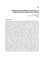
1. Introduction
Using porous media to extend the heat transfer area, improve effective thermal
conductivity, mix fluid flow and thus enhance heat transfer is an enduring theme in the field
of thermal fluid science. According to the internal connection of neighbouring pore
elements, porous media can be classified as the consolidated and the unconsolidated. For
thermal purposes, the consolidated porous medium is more attractive as its thermal contact
resistance is considerably lower. Especially with the development of co-sintering technique,
the consolidated porous medium made of metal, particularly the metallic porous medium,
gradually exhibits excellent thermal performance because of many unique advantages such
as low relative density, high strength, high surface area per unit volume, high solid thermal
conductivity, and good flow-mixing capability (Xu et al., 2011b). It may be used in many
practical applications for heat transfer enhancement, such as catalyst supports, filters, bio-
medical implants, heat shield devices for space vehicles, novel compact heat exchangers,
and heat sinks, et al. (Banhart, 2011; Xu et al., 2011a, 2011b, 2011c).
The metallic porous medium to be introduced in this chapter is metallic foam with cellular
micro-structure (porosity greater than 85%). It shows great potential in the areas of acoustics,
mechanics, electricity, fluid dynamics and thermal science, especially as an important
porous material for thermal aspect. Principally, metallic foam is classified into open-cell
foam and close-cell foam according to the morphology of pore element. Close-cell metallic
foams are suitable for thermal insulation, whereas open-cell metallic foams are often used
for heat transfer enhancement. Open-cell metallic foam is only discussed for thermal
performance. Figure 1(a) and 1(b) show the real structure of copper metallic foam

(a) (b)
Fig. 1. Metallic foams picture: (a) sample; (b) SEM (scanning electron microscope)

Heat Transfer – Engineering Applications

172
and its SEM image respectively It can be noted that metallic foams own three-dimensional
space structures with interconnection between neighbouring pore elements (cell). The
morphology structure is defined as porosity (

) and pore density (

), wherein pore
density is the pore number in a unit length or pores per inch (PPI).
In the last two decades, there have been continuous concerns on the flow and heat transfer
properties of metallic foam. Lu et al. (Lu et al., 1998) performed a comprehensive
investigation of flow and heat transfer in metallic foam filled parallel-plate channel using
the fin-analysis method. Calmidi and Mahajan (Calmidi & Mahajan, 2000) conducted
experiments and numerical studies on forced convection in a rectangular duct filled with
metallic foams to analyze the effects of thermal dispersion and local non-thermal
equilibrium with quantified thermal dispersion conductivity, k
d
, and interstitial heat transfer
coefficient, h
sf
. Lu and Zhao et al. (Lu et al., 2006; Zhao et al., 2006) performed analytical
solution for fully developed forced convective heat transfer in metallic foam fully filled
inner-pipe and annulus of tube-in-tube heat exchangers. They found that the existence of
metallic foams can significantly improve the heat transfer coefficient, but at the expense of

large pressure drop. Zhao et al. (Zhao et al., 2005) conducted experiments and numerical
studies on natural convection in a vertical cylindrical enclosure filled with metallic foams;
they found favourable correlation between numerical and experimental results. Zhao et al.
(Zhao & Lu et al., 2004) experimented on and analyzed thermal radiation in highly porous
metallic foams and gained favourable results between the analytical prediction and
experimental data. Zhao et al. (Zhao & Kim et al., 2004) performed numerical simulation
and experimental study on forced convection in metallic foam fully filled parallel-plate
channel and obtained good results. Boomsma and Poulikakos (Boomsma & Poulikakos,
2011) proposed a three-dimensional structure for metallic foam and obtained the empirical
correlation of effective thermal conductivity based on experimental data. Calmidi (Calmidi,
1998) performed an experiment on flow and thermal transport phenomena in metallic foams
and proposed a series of empirical correlations of fibre diameter d
f
, pore diameter d
p
,
specific surface area a
sf
, permeability K, inertia coefficient C
I
, and effective thermal
conductivity k
e
. Simultaneously, a numerical simulation was conducted based on the
correlations developed and compared with the experiment with reasonable results. Overall,
metallic foam continues to be a good candidate for heat transfer enhancement due to its
excellent thermal performance despite its high manufacturing cost.
For thermal modeling in metallic foams with high solid thermal conductivities, the local
thermal equilibrium model, specifically the one-energy equation model, no longer satisfies
the modelling requirements. Lee and Vafai (Lee & Vafai, 1999) addressed the viewpoint that

for solid and fluid temperature differentials in porous media, the local thermal non-
equilibrium model (two-energy equation model) is more accurate than the one-equation
model when the difference between thermal conductivities of solid and fluid is significant,
as is the case for metallic foams. Similar conclusions can be found in Zhao (Zhao et al., 2005)
and Phanikumar and Mahajan (Phanikumar & Mahajan, 2002). Therefore, majority of
published works concerning thermal modelling of porous foam are performed with two
equation models.
In this chapter, we report the recent progress on natural convection on metallic foam
sintered surface, forced convection in ducts fully/partially filled with metallic foams, and
modelling of film condensation heat transfer on a vertical plate embedded in infinite
metallic foams. Effects of morphology and geometric parameters on transport performance

Thermal Transport in Metallic Porous Media

173
are discussed, and a number of useful suggestions are presented as well in response to
engineering demand.
2. Natural convection on surface sintered with metallic porous media
Due to the use of co-sintering technique, effective thermal resistance of metallic porous
media is very high, which satisfies the heat transfer demand of many engineering
applications such as cooling of electronic devices. Natural convection on surface sintered
with metallic porous media has not been investigated elsewhere. Natural convection in an
enclosure filled with metallic foams or free convection on a surface sintered with metallic
foams has been studied to a certain extent (Zhao et al., 2005; Phanikumar & Mahajan, 2002;
Jamin & Mohamad, 2008).
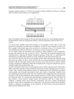
The test rig of natural convection on inclined surface is shown in Fig. 2. The experiment
system is composed of plexiglass house, stainless steel holder, tripod, insulation material,
electro-heating system, data acquisition system, and test samples. The dashed line in Fig. 2
represents the plexiglass frame. This experiment system is prepared for metallic foam
sintered plates. The intersection angle of the plate surface and the gravity force is set as the

inclination angle

. The Nusselt number due to convective heat transfer (with subscript
‘conv’) can be calculated as:





44
rad rad
conv
conv conv
ww
TTA
LL L
Nu h
kATTk ATT k




 
 

. (1)
where h, L, k,

, A, Tw, T


, E and

respectively denotes heat transfer coefficient, length,
thermal conductivity, heat, area, wall temperature, surrounding temperature, emissive
power and Boltzmann constant. The subscript ‘rad’ refers to ‘radiation’.
Meanwhile, the average Nusselt number due to the combined convective and radiative heat
transfer can be expressed as follows:

av av
w
()
LL
Nu h
kAT Tk




. (2)
In Eq.(2), the subscript ‘av’ denotes ‘average’.

6
0
°
Support Bracket
Right-Angle
Geometry
Data
Acqusition
DC

Power
Foam Sample
Film Heater
Korean Pine
Thermocouples
+
-
g
Plexiglass House
Insulation

Fig. 2. Test rig of natural convection on inclined surface sintered with metallic foams

Heat Transfer – Engineering Applications

174
Experiment results of the conjugated radiation and natural convective heat transfer on wall
surface sintered with open-celled metallic foams at different inclination angles are
presented. The metal foam test samples have the same length and width of 100 mm, but
different height of 10 mm and 40 mm. To investigate the coupled radiation and natural
convection on the metal foam surface, a black paint layer with thickness of 0.5 mm and
emissivity 0.96 is painted on the surface of the metal foam surface for the temperature
testing with infrared camera. Porosity is 0.95, while pore density is 10 PPI.
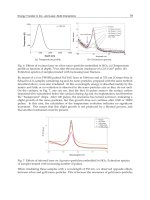
Figure 3(a) shows the comparison between different experimental data, several of which
were obtained from existing literature. The present result without paint agrees well with
existing experimental data (Sparrow & Gregg, 1956; Fujii T. & Fujii M., 1976; Churchil &
Ozoe, 1973). However, experimental result with paint is higher than unpainted metal foam
block. This is attributed to the improved emissivity of black paint layer of painted surface.
Figure 3(b) presents effect of inclination angle on the average Nusselt number for two
thicknesses of metallic foams (

/L

=0.1 and 0.4). As inclination angle increases from 0º
(vertical position) to 90º (horizontal position), heat transferred in convective model initially
increases and subsequently decreases. The maximum value is between 60º and 80º. Hence,
overall heat transfer increases initially and remains constant as inclination angle increases.
To investigate the effect of radiation on total heat transfer, a ratio of the total heat transfer
occupied by the radiation is introduced in this chapter, as shown below:

rad
R



. (3)
Figure 3(c) provides the effect inclination angle on R for different foam samples ( /L

=0.1
and 0.4). In the experiment scope, the fraction of radiation in the total heat transfer is in the
range of 33.8%–41.2%. For the metal foam sample with thickness of 10 mm, R is decreased as
the inclination angle increases. However, with a thickness of 40 mm, R decreases initially
and eventually increases as the inclination angle increases, reaching the minimum value of
approximately 75º.

0.0
4.0x10
7
8.0x10
7
1.2x10

8
1.6x10
15
30
45
60
75
Unpainted(E=0.78)
Fujii T. & Fujii M., 1976
Sparrow & Gregg, 1956
Churchil & Ozoe, 1973
Painted(E=0.96)
Nu
conv
Gr
*
Pr
Painted(E=0.96)
Unpainted(E=0.78)
-10 0 10 20 30 40 50 60 70 80 90 100
40
50
60
70
80
90
100
110
120
13

0
Nu
conv
Nu
av
Nu

/


/L=0.1


/L=0.1


/L=0.1


/L=0.4
-15 0 15 30 45 60 75 90 105
0.33
0.34
0.35
0.36
0.37
0.38
0.39
0.40
0.41

0.42



/L=0.1


/L=0.4
R

/

(a) (b) (c)
Fig. 3. Experimental results: (a) comparison with existing data; (b) effect of inclination angle
on heat transfer; (c) effect of inclination angle on R
Figure 4 shows the infrared result of temperature distribution on the metallic foam surface
with different foam thickness. It can be seen that the foam block with larger thickness has
less homogeneous temperature distribution.

Thermal Transport in Metallic Porous Media

175

(a) (b)
Fig. 4. Temperature distribution of metallic foam surface predicted by infrared rays: (a)
δ/L=0.1; (b) δ/L=0.4
3. Forced convection modelling in metallic foams
Research on thermal modeling of internal forced convective heat transfer enhancement using
metallic foams is presented here. Several analytical solutions are shown below as benchmark
for the improvement of numerical techniques. The Forchheimer model is commonly used for

establishing momentum equations of flow in porous media. After introducing several
empirical parameters of metallic foams, it is expressed for steady flow as:


2
ffffI
f
2
C
UU p U U UUJ
K
K





      



   
. (4)
where

,
p
,

, K, C

I
, U


is density, pressure, kinematic viscousity, permeability, inertial
coefficient and velocity vector, respectively. And J is the unit vector along pore velocity
vector
PP
/JU U

. The angle bracket means the volume averaged value. The term in the
left-hand side of Eq. (4) is the advective term. The terms in the right-hand side are pore
pressure gradient, viscous term (i.e., Brinkman term), Darcy term (microscopic viscous shear
stress), and micro-flow development term (inertial term), respectively. When porosity
approaches 1, permeability becomes very large and Eq. (4) is converted to the classical
Navier-Stokes equation.
Thermal transport in porous media owns two basic models: local thermal equilibrium
model (LTE) and local thermal non-equilibrium model (LNTE). The former with one-energy
equation treats the local temperature of solid and fluid as the same value while the latter has
two-energy equations taking into account the difference between the temperatures of solid
and fluid. They take the following forms [Eq. (5) for LTE and Eqs. (6a-6b) for LNTE]:


ff fe d
cU T k k T



 





. (5)



se s sf sf s f
0 kT haTT

   

. (6a)


ff f fe f sfsfs f
cU T k T ha T T

  



. (6b)

Heat Transfer – Engineering Applications

176
Subscripts ‘f’, ‘s’, ‘fe’, ‘se’, ‘d’ and ‘sf’ respectively denotes ‘fluid’, ‘solid’, ‘effective value of
fluid’, ‘effective value of solid’, ‘dispersion’ and ‘solid and fluid’.
T is temperature variable.

As stated above, Lee and Vafai (Lee & Vafai, 1999) indicated that the LNTE model is more
accurate than the LTE model when the difference between solid and fluid thermal
conductivities is significant. This is true in the case of metallic foams, in which difference
between solid and fluid phases is often two orders of magnitudes or more. Thus, LNTE
model with two-energy equations (also called two-equation model) is employed throughout
this chapter.
For modeling forced convective heat transfer in metallic foams, the metallic foams are
assumed to be isotropic and homogeneous. For analytical simplification, the flow and
temperature fields of impressible fluid are fully developed, with thermal radiation and
natural convection ignored. Simultaneously, thermal dispersion is negligible due to high
solid thermal conductivity of metallic foams (Calmidi & Mahajan, 2000; Lu et al., 2006;
Dukhan, 2009). As a matter of convenience, the angle brackets representing the volume-
averaging qualities for porous medium are dropped hereinafter.
3.1 Fin analysis model
As fin analysis model is a very simple and useful method to obtain temperature distribution,
fin theory-based heat transfer analysis is discussed here and a modified fin analysis method
of present authors (Xu et al., 2011a) for metallic foam filled channel is introduced. A
comparison between results of present and conventional models is presented.
Fin analysis method for heat transfer is originally adopted for heat dissipation body with
extended fins. It is a very simple and efficient method for predicting the temperature
distribution in these fins. It was first introduced to solve heat transfer problems in porous
media by Lu et al. in 1998 (Lu et al., 1998). As presented, the heat transfer results with fin
analysis exhibit good trends with variations of foam morphology parameters. However, it
has been pointed out that this method may overpredict the heat transfer performance. This
fin analysis method treats the velocity and temperature of fluid flowing through the porous
foam as uniform, significantly overestimating the heat transfer result. With the assumption
of cubic structure composed of cylinders, fin analysis formula of Lu et al. (Lu et al., 1998) is
expressed as:






2
s
sf
sf,b
2
sf
,
4
,0
Txy
h
Txy T x
kd
y






. (7)
where (x,y) is the Cartesian coordinates and d
f
is the fibre diameter. The subscript ‘f,b’
denotes ‘bulk mean value of fluid’.
In the previous model (Lu et al., 1998), heat conduction in the cylinder cell is only
considered and the surface area is taken as outside surface area of cylinders with thermal

conductivity k
s
. Based on the assumption, thermal resistance in the fin is artificially reduced,
leading to the previous fin method that overestimates heat transfer. Fluid with temperature
T
f,b
(x) flows through the porous channel. The fluid heat conduction in the foam is
considered together with the solid heat conduction. The effective thermal conductivity k
e

and extended surface area density of porous foam a
sf
instead of k
s
and surface area of solid
cylinders are applied to gain the governing equation. The modified heat conduction
equation proposed by present authors (Xu et al., 2011a) is as follows:

Thermal Transport in Metallic Porous Media

177





2
e,f
sf sf
e,f f,b

2
e
,
,0
Txy
ha
TxyTx
k
y






. (8)
Temperature T
e,f
(x) in Eq. (8) representing the temperature of porous foam is defined as the
equivalent foam temperature. With the constant heat flux condition, equivalent foam
temperature, and Nusselt number are obtained in Eq. (9) and Eq. (10):










e,f f,b w e
,cosh/sinhT x y T x q my mk mH




. (9)

   

ww
e
w f,b f e,f f,b f f
44
4tanh
,0
qq
k
HH
Nu mH mH
Tx T xk T x T xk k
 

. (10)
where q
w
is the wall heat flux and H is the half width of the parallel-plate channel. The fin
efficiency m is calculated with m=h
sf
a

sf
/k
e
.
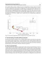
To verify the improvement of the present modified fin analysis model for heat transfer in
metallic foams, the comparison among the present fin model, previous fin model (Lu et al.,
1998), and the analytical solution presented in Section 3.2 is shown in Fig. 5. Figure 5(a)
presents the comparison between the Nusselt number results predicted by present modified
fin model, previous fin model (Lu et al., 1998), and analytical solution in Section 3.2.
Evidently, the present modified fin model is closer to the analytical solution. It can replace
the previous fin model (Lu et al., 1998) to estimate heat transfer in porous media with
improved accuracy. Only the heat transfer results of the present modified fin model and
analytical solution in Section 3.2 are compared in Fig. 5(b). It is noted that when k
f
/k
s
is
sufficiently small, the present modified fin model can coincide with the analytical solution.
The difference between the two gradually increases as k
f
/k
s
increases.


0.70.80.91.0
0
500
1000
1500

2000
2500
Nu

k
f
/k
s
=10
-4
k
f
/k
s
=10
-3
analytical model
present fin model
Lu et al., 1998

10
-7
10
-6
10
-5
10
-4
10
-3

10
-2
10
-1
10
0
10
1
10
2
10
3
N
u
k
f
/k
s
analytical model present fin model




=0.85




=0.90




=0.95
k
f
/k
s
=10
-4

(a) (b)
Fig. 5. Comparisons of Nu (a) among present modified fin model, previous fin model (Lu et
al., 1998), and analytical solution in Section 3.2.1 (

=10 PPI, H=0.005 m, u
m
=1 m·s
-1
); (b)
between present modified fin model and analytical solution in Section 3.2.1 (

=10 PPI,
H=0.005 m, u
m
=1 m·s
-1
)

Heat Transfer – Engineering Applications

178
3.2 Analytical modeling
3.2.1 Metallic foam fully filled duct
In this part, fully developed forced convective heat transfer in a parallel-plate channel filled
with highly porous, open-celled metallic foams is analytically modeled using the Brinkman-
Darcy and two-equation models and the analytical results of the present authors (Xu et al.,
2011a) are presented in the following. Closed-form solutions for fully developed fluid flow
and heat transfer are proposed.
Figure 6 shows the configuration of a parallel-plate channel filled with metallic foams. Two
infinite plates are subjected to constant heat flux q
w
with height 2H. Incompressible fluid
flows through the channel with mean velocity u
m
and absorbs heat imposed on the parallel
plates.

2H
x
y
o
q
w
q
w
u
m
Metallic Foams

Fig. 6. Schematic diagram of metallic foam fully filled parallel-plate channel
For simplification, the angle brackets representing volume-averaged variables are dropped
from Eqs. (4), (6a), and (6b). The governing equations and closure conditions are normalized
with the following qualities:

sw
fw
sf
mfm wsewse
d
,, , ,
d/ /
yp
TT
uK TT
YU P
Hu ux
q
Hk
q
Hk




    , (11a)


2
fe sf sf

f
2
se se se
,,, ,/, 1/
khaH
Kk
Da B C D s Da t D C C
kk k
H

  . (11b)
Empirical correlations for these parameters are listed in Table 1.
After neglecting the inertial term in Eq. (4), governing equations for problem shown in Fig. 6
can be normalized as:

2
2
2
()0
U
sU P
Y




. (12a)

2
s

sf
2
()0D
Y






. (12b)

2
f
sf
2
()CD U
Y






. (12c)

Thermal Transport in Metallic Porous Media

179
Parameter Correlation Reference

Pore diameter
p
d
p
0.0254 /d


Calmidi,
1998
Fibre diameter
f
d
 

1
fp
1.18 1 / 3 1 exp 1 /0.04dd
 



   



Calmidi,
1998
Specific surface area
sf
a





2
1 /0.04
sf f p
31 /0.59ade d








Zhao
et al., 2001
Permeability
K



1.11
0.224
2
fp p
0.00073 1 /Kddd





Calmidi,
1998
Local heat transfer
coefficient
sf
h



0.4 0.37
df d
0.5 0.37 3
sf d f d
0.6 0.37 3 5
df d
0.76 / , 1 40
0.52 / , 40 10
0.26 / , 10 2 10
Re Pr k d Re
hRePrkdRe
Re Pr k d Re











df f
/Re ud



Lu
et al., 2006
Effective thermal
conductivity
e
k




A
22
sf
4
21 421
R
eekeek

 




 

2
B
22
sf
2
2242
e
R
eeke eek







 

2
C
22
sf
22
2 1 22 2 2 2 1 22
e
R
ek e e k
 





D
22
sf
2
4
e
R
ek e k







3
22 5/8 2 2
342
e
ee







, 0.339e



e
ABCD
1
2
k
RRRR



f
se e
0
k
kk

 ,
s
fe e
0
k
kk


Boomsma
&
Poulikakos,

2001
Table 1. Semi-empirical correlations of parameters for metallic foams
The dimensionless closure conditions can likewise be derived as follows:

s
f
sf
0, 0; 1, 0, 0.
U
YYU
YYY







 


(13)
Thus, the dimensionless velocity profile is expressed by the hyperbolic functions:



cosh( ) /cosh( ) 1UP sY s

 . (14a)

1
tanh( ) / 1
P
ss


. (14b)

Heat Transfer – Engineering Applications

180
Meanwhile, dimensionless fluid and solid temperatures can be derived as follows:

2
sf
22
cosh( ) 1 1 1
22
cosh( )
sY
CP Y
ss s



  







. (15a)

 








2
2
f
2
2
2
2
2
1/
cosh
cosh( )
cosh( ) cosh( )
1
11
1/2 1/ 1/ 1
1
21 1

Ds
sY
Cs tY
P
ts
Cs DC
DC C s DC
DsC
Y
CDC









 












. (15b)

 







22 2
s
2
2
2
2
2
cosh cosh
/
cosh( ) cosh( )
1
11
1/2 1/ / 1
1
21 1
tY sY
Cs Ds
P
ts

Cs DC
DC C s DC
DsCC
Y
CDC




 



 











. (15c)
The dimensionless numbers, friction factor f, and Nusselt number Nu are shown below.

2
fm

d/d 4
32
/2
pxH
P
f
Re Da
u




. (16a)

w
w f,b f f,b
44
q
H
Nu
TTk B



. (16b)
In Eq. (20), the dimensionless bulk fluid temperature can be obtained using Eq. (19).

 
  



2
f
1
2
f,b f
2
2
0
22 2
2
222
cosh cosh
1
d
d
1
2 1 1 cosh cosh
d
22 22
11 1
1cosh2
4(1)cosh 4
A
A
ss
st st
Cs
UA
st st

A
UYP
DC C s DC s t
UA
A
D
D
ee
s
ss
ss s
s
Cs DC s s Cs




 

















  



  



  
  
 

   





 

 

 

2
22

22
22
2
2
22
(1)cosh
11
21
11 11
11 1
1
1
21
61 1
1cosh
DC s s
Cs Cs
sC
DC C s DC DC C s DC t
D
D
C
s
s
CDC
Cs DC s







  


 
 
 










 



 




. (17)

Thermal Transport in Metallic Porous Media

181
The Nusselt number of the present analytical solution is compared with experiment data
(Zhao & Kim, 2001) for forced convection in rectangular metallic foam filled duct [Fig. 7(a)].
As illustrated, the difference between the analytical and previous experiment results is
attributed to the experimental error and omission of the dispersion effect and quadratic term
in the velocity equation. Overall, the analytical and experimental results are correlated with
each other, with reasonable similarities. To examine the effect of the Brinkman term,
comparison between temperature profiles of the present solution and that of Lee and Vafai
(Lee & Vafai, 1999) is presented in Fig. 7(b). It can be observed that temperature profiles of
the two solutions are similar. In particular, the predicted temperatures for solid and fluid of
Lee and Vafai (Lee & Vafai, 1999) are closer to the wall temperature than the present
solution. This is due to the completely uniform cross-sectional velocity assumed for the
Darcy model by Lee and Vafai (Lee & Vafai, 1999). The comparison provides another
evidence for the feasibility of the present solution.

012345678
0
100
200
300
400
500
Zhao & Kim, 2001
present analytical solution
Nu
Sam
p
le No.
=0.943 0.857 0.939 0.898 0.910 0.919 0.911

= 10 10 30 30 60 30 30 PPI
-1.0 -0.5 0.0 0.5 1.0
-0.8
-0.6
-0.4
-0.2
0.0
fluid

Y
Lee & Vafai, 1999
present analytical solution
solid

(a) (b)
Fig. 7. Validation of present solution: (a) compared with the experiment; (b) compared with
Lee and Vafai (Lee & Vafai, 1999) (

=0.9,

=10 PPI, H=0.01 m, u
m
=1 m/s, k
f
/k
s
=10
-4
)
Figure 8(a) displays velocity profiles for smooth and metallic foam channels with different

porosities and pore densities from the analytical solution for velocity in Eq. (14a). The
existence of metallic foams can dramatically homogenize the flow field and velocity
gradient near the impermeable wall because the metallic foam channel is considerably
higher than that for the smooth channel. With decreasing porosity and increasing pore
density, the flow field becomes more uniform and the boundary layer becomes thinner. This
implies that high near wall velocity gradient, created by the ability to homogenize flow field
for metallic foams, is an important reason for heat transfer enhancement.
Figure 8(b) shows the effect of porosity on the temperature profiles of solid and fluid
phases. Porosity has significant influence on both solid and fluid temperatures. When
porosity increases, temperature difference between the solid matrix and channel wall is
improved. This is because the solid ligament diameter is reduced with increasing porosity
under the same pore density, which results in an increased thermal resistance of heat
conduction in solid matrix. In addition, the temperature difference between the fluid and
channel wall has a similar trend. This is attributed to the reduction of the specific surface

Heat Transfer – Engineering Applications

182
area caused by increasing porosity to create higher heat transfer temperature difference
under the same heat transfer rate.
Figure 8(c) illustrates the effect of pore density on temperature profile. It is found that
sse
/ k

almost remains unchanged with increasing pore density since effective thermal
conductivity and thermal resistance in solid matrix are affected not by pore density but by
porosity. While
fse
/ k


increases with an increase in pore density, it shows that temperature
difference between fluid and solid wall is reduced since the convective thermal resistance is
reduced due to the extended surface area.

0.0 0.2 0.4 0.6 0.8 1.0 1.2 1.4
-1.0
-0.5
0.0
0.5
1.0
Analytical solution
Y
U
smooth channel


=0.80,

=10 PPI


=0.95,

=10 PPI


=0.95,

=60 PPI
-0.3 -0.2 -0.1 0.0

-1.0
-0.5
0.0
0.5
1.0
Y

/k
se
( m·K·W
-1
)

=0.95

=0.85

s
/k
se

f
/k
se
Analytical solution
-0.015 -0.010 -0.005 0.000
-1.0
-0.5
0.0
0.5

1.0

f
/k
se
, 60 PPI

s
/k
se
, 20 PPI

f
/k
se
, 20 PPI
Y

/k
se
( m·K·W
-1
)

s
/k
se
, 60 PPI
Analytical solution

(a) (b) (c)
Fig. 8. Effect of metallic foam morphology parameters on velocity and temperature profiles:
(a) velocity profile (H=0.005 m); (b) temperature profile affected by porosity
(

=10 PPI, H=0.01 m, u
m
=5 m·s
-1
, k
f
/k
s
=10
-4
); (c) temperature profile affected by pore density
(

=0.9, H=0.01 m, u
m
=5 m·s
-1
, k
f
/k
s
=10
-5
)
3.2.2 Metallic foam partially filled duct

In the second part, fully developed forced convective heat transfer in a parallel-plate
channel partially filled with highly porous, open-celled metallic foam is analytically
investigated and results proposed by the present author (Xu et al., 2011c) is presented in this
section. The Navier-Stokes equation for the hollow region is connected with the Brinkman-
Darcy equation in the foam region by the flow coupling conditions at the porous-fluid
interface. The energy equation for the hollow region and the two energy equations of solid
and fluid for the foam region are linked by the heat transfer coupling conditions. The
schematic diagram for the corresponding configuration is shown in Fig. 9. Two isotropic

2H
x
y
q
w
q
w
u
m
2y
i
Hollow region
Metallic foams
Metallic foams
o

Fig. 9. Schematic diagram of a parallel-plate channel partially filled with metallic foam

Thermal Transport in Metallic Porous Media

183

and homogeneous metallic foam layers are symmetrically sintered on upper and bottom
plates subjected to uniform heat flux. Fluid is assumed to possess constant thermal-physical
properties. Thermal dispersion effect is neglected for metallic foams with high solid thermal
conductivity (Calmidi & Mahajan 2000). To obtain analytical solution, the inertial term in
Eq.(4) is neglected as well.
For the partly porous duct, coupling conditions of flow and heat transfer at the porous-fluid
interface can be divided into two types: slip and no-slip conditions. Alazmi and Vafai
(Alazmi & Vafai, 2001) reviewed different kinds of interfacial conditions related to velocity
and temperature using the one-equation model. It was indicated that the difference between
different interfacial conditions for both flow and heat transfer is minimal. However, for heat
transfer, since the LTNE model is more suitable for highly conductive metallic foams rather
than the LTE model, the implementation of LTNE model on thermal coupling conditions at
the foam-fluid interface is considerably more complex in terms of number of temperature
variables and number of interfacial conditions compared with LTE model. The momentum
equation in the fluid region belongs to the Navier-Stokes equation while that in the foam
region is the Brinkman-extended-Darcy equation, which is easily coupled by the flow
conditions at foam-fluid interface.
For heat transfer, Ochoa-Tapia and Whitaker (Ochoa-Tapia & Whitaker, 1995) have
proposed a series of interface conditions for non-equilibrium conjugate heat transfer at the
porous-fluid interface, which can be used for thermal coupling at the foam-fluid interface of
a domain party filled with metallic foams. Given that the two sets of governing equations
are coupled at the porous-fluid interface, the interfacial coupling conditions must be
determined to close the governing equations. Continuities of velocity, shear stress, fluid
temperature, and heat flux at the porous-fluid interface should be guaranteed for
meaningful physics. The corresponding expressions are shown in Eqs. (18)–(21):

-+
ii
yy
uu . (18)

-+
ii
f
f
dd
dd
yy
uu
y
y



 . (19)

-+
ii
ff
yy
TT . (20)

-
+
i
i
s
ff
ffese
y

y
T
TT
kkk
yyy







. (21)
There are three variables for two-energy equations: the fluid and solid temperatures of the
foam region and the temperature of the open region. Therefore, another coupling condition
is required to obtain the temperature of solid and fluid in the foam region (Ochoa-Tapia &
Whitaker, 1995), as:



-
+
i
ii
se s sf s f
y
yy
kT hT T

  . (22)

For the reason that axial heat conduction can be neglected, Eq. (22) is simplified as follows:

Heat Transfer – Engineering Applications

184



-
+
i
i
i
s
se sf s f
y
y
y
T
khTT
y




. (23)
Due to the fact that the solid ligaments are discontinuous at the foam-fluid interface, heat
conduction through the solid phase is totally transferred to the fluid in the manner of
convective heat transfer across the foam-fluid interface. Thus, the physical meaning of
Eq.(22) stands for the convective heat transfer at the foam-fluid interface from the solid

ligament to the fluid nearby. Thus, the governing equations in the foam region and that in
the fluid region are linked together via these interfacial coupling conditions.
With the dimensionless qualities in Eqs.(11a)–(11b) and the following variables,

sf
se
,
i
i
y
hH
YA
Hk

. (24)
governing equations for the fluid region and the foam region are normalized. Dimensionless
governing equations for the hollow region (
i
0 YY

 ) are as follows:

2
2
0
UP
Da
Y





. (25)

2
f
2
1
U
B
Y




. (26)
Dimensionless governing equations for the foam region (
i
1YY

 ) are as follows:


2
2
2
0
U
sUP
Y





. (27)


2
s
sf
2
0D
Y






. (28)


2
f
sf
2
CD U
Y







. (29)
Corresponding dimensionless closure conditions are as follows:

f
0: 0
U
Y
YY





. (30a)

sf
1: 0, 0YU



. (30b)
When
i
YY , the dimensionless coupling conditions are as follows:

-+

ii
YY
UU . (31a)

Thermal Transport in Metallic Porous Media

185

-+
ii
1
YY
dU dU
dY dY

 . (31b)

-+
ii
ff
YY

 . (31c)

-
+
i
i
s
ff

Y
Y
BC
YYY









. (31d)



-
+
i
i
+
i
s
sf
Y
Y
Y
A
Y






. (31e)
The velocity field is typically obtained ahead of the temperature field for the uncoupled
relationship between the momentum and energy equations. With closure conditions for
flow in Eqs. (30a), (30b), (31a), and (31b), the dimensionless velocity equation of Eqs. (25)
and (27) can be solved and the solution for velocity is as follows:


2
0i
12 i
1
,0
2
1, 1
sY sY
PYC YY
Da
U
PCe Ce Y Y














. (32)
where dimensionless pressure drop P , constants
C
0
, C
1
, and C
2
are as follows:


3
i
12 0i
1
1
1
6
ss
P
Y
Ce Ce CY
sDa





. (33a)



ii
2
01 2 i
/2 1
sY sY
CCe Ce Y Da


 . (33b)

 
ii
ii
i
1
11
sY sY
sY sY
esYe
C
ee






. (33c)

 
i
ii
i
2
11
sY
s
sY sY
esYe
C
ee




. (33d)
The solution to the energy equations is as follows:





42

0
3i
2
67 12
2
f
i
2
5
4
2
11
,0
24 2
1/
1
,1
11
21 1 1
1
tY tY sY sY
C
PYYC YY
BDa
Ds
Ce Ce Ce Ce
Cs DC
PYY
C
C

YY
CCC
DC




 








 
 

 
















. (34a)

Heat Transfer – Engineering Applications

186






2
67 12
2
s i
2
5
4
2
1/
1
,1
1
21 1 1
1

tY tY sY sY
Ds
Ce Ce Ce Ce
C
Cs DC
PYY
C
CC
YY
CCC
DC



 

 









(34b)
The constants in the above equation are defined as follows:






ii ii
2
67 12
2
42
0
3 ii
2
5
4
ii
2
1/
1
1
11242
21 1 1
1
tY tY sY sY
Ds
Ce Ce Ce Ce
Cs DC
C
CB Y Y
C
CDa
YY

CCC
DC



 

 









. (35a)

3
4i0i
1
6
CYCY
Da

. (35b)

54
2

11
2
CC
s
 
. (35c)







i
ii
89
6
11
1
11
tY
t
tY tY
AC Ct e C e C
C
AC Ct e AC Ct e



 



 

 
. (35d)







i
ii
98
7
11
1
11
tY
t
tY tY
eC A C Ct e C
C
AC Ct e AC Ct e

   



 

 
. (35e)

 
2
8
2
2
11
Cs
C
DC C s DC







. (35f)



 
ii
2
12 i 4
9

2
2
1
11
1
11
sY sY
Ce Ce C s Y C
CA
DC C
Cs DC
CCsDC




   




 





. (35g)
The bulk dimensionless fluid temperature is expressed as follows:
 



 



 



 


i
i
ii i
i
22
f
1
752
03
i
f,b f f i i 0 0 3 i
2
0
2
16 26
17
2

2
2
27 11
1
d
7
1
d
1
120 6
336
d
2
Y
A
Y
A
st stY st stY st stY
st stY
s
UA
CC
PY
A
UY UdY Y Y C CCY
BDaDa
Da
UA
A
CC CC

CC
Pee ee ee
st st st
CC NC
ee ee
st s


  
 


 
















ii

i
i
2
2
2
12
2
33
122 22
23142i3i14
22
2
3 3
222 22
23142i3i14
2 2
2
22 2 2
22 2 2
sY sY
s
sY
s
sY
s
NC
ee
s
NN
CNN NN

eN N N N e NY N Y N N
sss s s
ss
NN
CNN NN
eNN N N e NY N YN N
sss s s
ss





 



        
 






 



       










ii
32
6337
ii1124i
112 1
32
tY tY
tt
CNN
C
ee e e Y Y NCCN Y
tt


 
 


 

   



(36)

Thermal Transport in Metallic Porous Media

187
In Eq. (36), the constants N
1
, N
2
, N
3
, and N
4
are as follows:


2
1
2
1/
1
Ds
N
Cs DC





,

2
1
21
N
C


,
4
3
1
C
N
C


,

4
2
1
1
N
DC


. (37)
Friction factor

f and Nusselt number Nu are the same with Eqs. (16a) and (16b).
Velocity profiles predicted by the analytical solutions shown in Eq. (32) at three
combinations of porosity and pore density are presented in Fig. 10(a). It is found that
velocity in the hollow space is considerably higher than that in the foam region with
obstructing foam ligaments. Increasing porosity or decreasing pore density can both
increase velocity in foam region and decrease velocity in open region simultaneously since
flow resistance in the foam region can be reduced by increasing porosity and decreasing
pore density of metallic foams. Figure 10(b) illustrates the comparison of velocity profiles for
four hollow ratios: 0 (foam fully filled channel), 0.2, 0.5, 0.8, and 1.0 (smooth channel). The
velocity profile is a parabolic distribution for the smooth channel and the profile for fully
filled channel is similar, except that the distribution is more uniform since no sudden
change of permeability is in the cross section. Comparatively for the foam partially filled
channel, sudden change in permeability occurs at the porous-fluid interface; the average
velocity in the central fluid region for foam partially filled channel (
Y
i
=0.2, 0.5, 0.8) is higher
than those of the foam fully filled channel and empty channel. Moreover, maximum velocity
in the central region decreases with the increase in hollow ratio due to the sizeable
difference in permeability between porous and clear fluid regions. Velocity in the foam
region of foam partially filled channel is considerably lower than those of foam fully filled
channel and smooth channel.

-1.0 -0.8 -0.6 -0.4 -0.2 0.0 0.2 0.4 0.6 0.8 1.0
0
1
2
3
4
5

U
Y

=0.85,

=10 PPI

=0.85,

=30 PPI

=0.95,

=10 PPI
Y
i
=0.3
-1.0 -0.8 -0.6 -0.4 -0.2 0.0 0.2 0.4 0.6 0.8 1.0
0
1
2
3
4

=0.9

=10 PPI
H=0.005 m
Y
i

=0.8
Y
i
=0.5
U
Y
i
=0.2
Y
i
=1
Y
i
=0
Y

(a) (b)
Fig. 10. Effect of key parameters on velocity profiles: (a) metal foam morphology
parameters; (b) hollow ratio
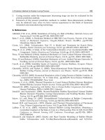
Figure 11(a) presents the influence of porosity on temperature profile. Evidently, the
nominal excess temperature of fluid in the hollow region decreases in the
y direction and the
decreasing trend becomes less obvious in the foam region. This is due to the total thermal
resistance in the foam region, which is lower than that in the hollow region for the
significant heat transfer surface extension. The nominal excess temperatures of fluid and

Heat Transfer – Engineering Applications

188
solid in the foam region for


=0.9 were lower than that for

=0.95 because decreased
porosity leads to the increase in both the effective thermal conductivity and the foam surface
area to improve the corresponding heat transfer with the same heat flux. Effect of pore
density on temperature profile is shown in Fig. 11(b). The solid excess temperature is almost
the same in the foam region for different pore densities. This is attributed mainly to the
effect of porosity on heat conduction thermal resistance of the foam, as shown in Table 1. On
the other hand, the nominal excess fluid temperature of 5 PPI is significantly smaller than
that of 30 PPI. The trend inconsistency of the fluid and solid temperatures in the two regions
for the two pore densities is caused by mass flow fraction in the foam region. The local
convective heat transfer coefficient for 5 PPI was higher than 30 PPI due to the relative
higher mass flow fraction in the foam region.
However, the heat transfer surface area inside the foam of 5 PPI is lower than that of 30 PPI.
The two opposite effects competed with each other, resulting in the identical temperature
difference between wall and fluid in the foam region. However, in the hollow region, the
porous-fluid interface area becomes the only surface area where porosity for the two pore
densities is the same. Hence, the temperature difference between wall and fluid for 5 PPI is
reduced and obviously lower than that for 30 PPI.
Figure 11(c) presents the comparison between fluid and solid temperature distribution for
different channels, including empty channel (
Y
i
=1), foam partially filled channel (Y
i
=0.5),
and foam fully filled channel (
Y
i

=0). The nominal excess temperature becomes dependent
on the heat transfer area and local heat transfer coefficient. In the hollow region, the heat
transfer surface area is reduced to the interface area for the foam partially filled channel
(
Y
i
=0.5), which was considerably smaller than the volume surface area of the fully filled
channel (
Y
i
=0). The nominal fluid excess temperature increases in the order of Y
i
=1,
Y
i
=0.5, and Y
i
=0 since the total convective thermal resistance 1/(h
sf
a
sf
) decreases in the
order
Y
i
=0, Y
i
=0.5, Y
i
=1 in the clear fluid region. In the near-wall foam region, local heat

transfer coefficient for
Y
i
=0.5 is reduced compared with that for Y
i
=0. However, the effect
of fluid heat conduction dominates in the near-wall area, resulting in a lower nominal
fluid excess temperature for
Y
i
=0.5 compared with that for the foam fully filled channel
(
Y
i
=0). Thus, an intersection point occurs in the curve of the fluid excess temperature
distribution.

-1.0 -0.8 -0.6 -0.4 -0.2 0.0 0.2 0.4 0.6 0.8 1.0
0
1
2
3
4
5
6
7
8
fluid
solid


=5 PPI
Re=1500
H=0.01 m
k
f
/k
s
=10
-3
Y
i
=0.3
(
T
w
-
T
)
/
(
q
w
H
)
m·K·W
-1
Y


=0.9


=0.95
-1.0 -0.8 -0.6 -0.4 -0.2 0.0 0.2 0.4 0.6 0.8 1.0
0
2
4
6
8
10
solid

=0.95
Re=1500
H=0.01 m
k
f
/k
s
=10
-3
Yi=0.3
(
T
w
-
T
) /( q
w
H)

m·K·W
-1
Y


=5 PPI


=30 PPI
fluid
-1.0 -0.8 -0.6 -0.4 -0.2 0.0 0.2 0.4 0.6 0.8 1.0
10
-3
10
-2
10
-1
10
0
10
1
10
2
( T
w
-T) /(q
w
H)
m·K·W
-1

Y
Y
i
=0
Y
i
=0.5
Y
i
=1
solid
fluid

=0.95

=10 PPI Re=1500
H=0.01 m
k
f
/k
s
=10
-4


(a) (b) (c)
Fig. 11. Effects of key parameters on temperature profiles: (a) porosity; (b) pore density; (c)
hollow ratio
Figure 12(a) presents the effect of porosity on
Nu for four different metal materials: steel,

nickel, aluminum, and copper with air as working fluid. The
Nusselt number does not

Thermal Transport in Metallic Porous Media

189
monotonically increase with porosity increase and a maximum value of Nu exists at a
critical porosity. This can be attributed to the fact that increasing porosity will lead to a
decrease in effective thermal conductivity and an increase in mass flow rate in the foam
region. Below the critical porosity, the increase in the mass flow region prevails and
Nu
increases to the maximum value. When porosity is higher than the critical value, which
approaches 1, the decrease in thermal conductivity prevails. The Nusselt number sharply
reduces and approaches the value of the smooth channel.
It is observed that the increase in the solid thermal conductivity can result in an increase in
Nu. The critical porosity likewise increases with the solid thermal conductivity. It is implied
that porosity should be maintained at an optimal value in the design of related heat transfer
devices to maximize the heat transfer coefficient. Figure 12(b) shows the effect of pore
density on
Nu for different hollow ratios in which the two limiting cases for Y
i
=1 (J.H.
Lienhard IV & J.H. Lienhard V, 2006) and
Y
i
=0 (Mahjoob & Vafai, 2009) are compared as
references. As
Y
i
approaches 1, the predicted Nu of the present analytical solution, with a

value of 8.235, coincides accurately with that of the smooth channel (J.H. Lienhard IV & J.H.
Lienhard V, 2006). As
Y
i
approaches 0, the difference between the present analytical result
and that of Mahjoob and Vafai (Mahjoob & Vafai, 2009) is very mild since the effect of
viscous force of impermeable wall is considered in the present work and not considered in
the research of Mahjoob and Vafai (Mahjoob & Vafai, 2009) with the Darcy model. This
provides another evidence for feasibility of present analytical solution.
Moreover, it is found that the
Nusselt number gradually decreases to a constant value as
pore density increases. Increasing pore density can improve the heat transfer surface area
but lead to drastic reduction in mass flow rate in the foam region. Hence, small pore density
is recommended to maintain heat transfer performance and to reduce pressure drop for
thermal design of related applications. The effect of hollow ratio on
Nu under various k
f
/k
s

is shown in Fig. 12(c). At high
k
f
/k
s
(1, 10
-1
), a minimized Nu exists as Y
i
varies from 0 to 1,

which is in accordance with the thermal equilibrium result of Poulikakos and Kazmierczak
(Poulikakos & Kazmierczak, 1987). However,
Nu monotonically decreases as Y
i
varies from
0 to 1 for low
k
f
/k
s
, as in the case of metallic foams with high solid thermal conductivities.
This is attributed to the fact that both the mass flow rate and foam surface area in the foam
region are reduced as
Y
i
increases. As Y
i
approaches 1, the Nusselt number gradually
converges to the value 8.235, which is the exact value of forced convective heat transfer in
the smooth channel (
Y
i
=1).

0.70 0.75 0.80 0.85 0.90 0.95 1.00
15
20
25
30
35

40
45
nickel
Nu

steel
aluminum
copper

=10 PPI
H=0.005 m
Re=1500
k
f
=0.0276W·m
-1
·K
-1
Y
i
=0.3
10 20 30 40 50 60
10
100
H=0.01 m Re=1500
k
f
/k
s
=10

-3

=0.9
Nu

PPI
Y
i
? 0, present Y
i
=0.1, present
Y
i
=0.3, present Y
i
=0.5, present
Y
i
=0.7, present Y
i
=0.9, present
Y
i
? 1, present Y
i
=0, Mahjoob & Vafai, 2009
Y
i
=1, J.H. Lienhard IV & J.H. Lienhard V, 2006
0.0 0.2 0.4 0.6 0.8 1.0

10
100

=0.9

=10 PPI
Re=1500
H=0.01 m
Nu
Y
i
k
f
/k
s
=1
k
f
/k
s
=10
-1
k
f
/k
s
=10
-2
k
f

/k
s
=10
-3
8.235

(a) (b) (c)
Fig. 12. Effects of key parameters on Nu: (a) porosity; (b) pore density; (c) hollow ratio

Heat Transfer – Engineering Applications

190
3.3 Numerical modeling for double-pipe heat exchangers
In this section, the two-energy-equation numerical model has been applied to parallel flow
double-pipe heat exchanger filled with open-cell metallic foams. The numerical results of
the present authors (Du et al., 2010) are introduced in this section. In the model, the solid-
fluid conjugated heat transfer process with coupling heat conduction and convection in the
open-celled metallic foam, interface wall, and clear fluid in both inner and annular space in
heat exchanger is fully considered. The non-Darcy effect, thermal dispersion (Zhao et al.,
2001), and wall thickness are taken into account as well.
Figure 13 shows the schematic diagram of metal foam filled double-pipe heat exchanger
with parallel flow, in which the cylindrical coordinate system and adiabatic boundary
condition in the outer surface of the annular duct are shown. The interface-wall with
thickness
δ
is treated as conductive solid block in the internal part of metallic foams. R
1
, R
2
,

and
R
3
represent the inner radius of the inner pipe, outer radius of the inner pipe, and inner
radius of the outer pipe, respectively. Fully developed conditions of the velocity and
temperature at the exit are adopted. For simplification, incompressible fluids with constant
physical properties are considered. Metallic foams are isotropic, possessing no contact
resistance on the interface wall.

R
2
R
1
R
3
r
x
0

Fig. 13. Schematic diagram of double-pipe heat exchanger with parallel flow
With the Forchheimer flow model for momentum equation and two-equation model for
energy equations, the flow and heat transfer problem shown in Fig. 13 is described with the
following governing equations:
Continuity equation:

ff
()1( )
0
urv
xrr






. (38)
Momentum equations:

2 222
2
ff ffI
ff
()1( ) 1
()( )
p
uruv u u Cu
ru
xrr xx xrr rK
K
 
 

 
  

. (39a)

2222
2
ff ffI

ff
()1( ) 1
()( )
p
uv r v v v C v
rv
xrr rx xrr rK
K
 
 

 
  

. (39b)
Two energy equations:

Thermal Transport in Metallic Porous Media

191

ss
se se sf sf s f
1
()0
TT
krkhaTT
xxrr r



 


 
  
 
. (40a)

fe d fe d sf sf
ff ff f f
sf
fff
()1( ) 1
()
kk kk ha
uT r vT T T
rTT
xrr xcxrrcr c

 


  
 
 
 
. (40b)
where
x and r pertain to cylindrical coordinate system. The tortuous characteristic of fluids
in metallic foams enhances heat transfer coefficients between fluid and solid, influence of

which is considered by introducing dispersion conductivity
k
d
(Zhao et al., 2001).
In the interfacial wall domain, the conventional two-equation model cannot be directly
used since no fluid can flow through the wall. Hence, particular treatments are proposed
to take into account the interface wall. Special fluids can be assumed to exist in the
interface wall such that the fluid-phase equation in Eq. (40b) can be applied. However, the
dispersion conductivity
k
d
is considered to be zero and the viscosity of fluid can be
considered to be infinite, thus leading to zero fluid velocity. As such, the temperature and
efficient thermal conductivity of the special fluid and solid are the same, that is to say,
T
s
=T
f
, k
fe
=k
se
. In this condition, Eqs. (40a) and (40b) are unified into one for the interface
wall, as seen in Eq. (41):

ss
se se
1
0
TT

krk
xxrr r


 


 
  
 
. (41)
According to this extension, the temperature and wall heat flux distribution can be
determined by Eq. (43a) during the iteration process, instead of being described as a
constant value in advance. Due to the continuity of the interfacial wall heat flux, the inner
side wall heat flux
q
inner
and the annular side wall heat flux q
annular
are formulated in Eq.
(42).

inner annular
2
1
0
R
qq
R


. (42)
where
q is the heat flux and the subscripts ‘inner’ and ‘annular’ respectively denotes
physical qualities relevant to the inner-pipe and the annular space. Simultaneously heat
transfer through solid and fluid at the wall can be obtained using the method formulated by
Lu and Zhao et al. (Lu et al., 2006; Zhao et al., 2006), which is frequently used and validated
in relevant research. The two heat fluxes are expressed as:

1
s
f
inner se fe
rR
T
T
qkk
rr








(inner side) (43a)

2
s
f

annular se fe
rR
T
T
qkk
rr




 



(annular side) (43b)
Conjugated heat transfer between heat conduction in the interfacial wall and metal
ligament, as well as the convection in the fluid, are solved within the entire computational
domain.

Heat Transfer – Engineering Applications

192
On the center line of the double-pipe heat exchanger, symmetric conditions are adopted.
No-slip velocity and adiabatic thermal boundary conditions for the outside wall of the heat
exchanger are conducted as well. Since the wall is adiabatic, the heat flux equals to zero
when temperatures of the fluid and solid matrices are equivalent. At the entrance of the
double pipe, velocities and fluid temperatures in both flow passages are given as uniform
distribution profiles, while the gradient of the metallic foam temperature is equal to zero,
according to Lu and Zhao et al. (Lu et al., 2006; Zhao et al., 2006). Fully developed
conditions are adopted at the outlet. For the interface wall, velocity of the fluid is zero, as

previously determined, which indicates that dynamic viscosity is infinite. The specifications
of the boundary conditions are shown in Table 2. Both governing equations are described
using the volume-averaging method. During code development, the two equations are
unified over the entire computational domain. The above special numerical treatment is
implemented in the wall domain.


x-velocity u y-velocity v
Fluid temperature
f
T Solid temperature
s
T
0x 
in
uu


0v


ff,in
TT


s
0
T
x





xL
0
u
x




0
v
x




f
0
T
x




s
0
T
x





0r 
0
u
r




v =0
f
0
T
r




s
0
T
r




12

RrR
0u

0v


sf
TT


sf
TT
3
rR
0u

0v


s
f
fe se
0
T
T
qk k
rr






,
sf
TT
Table 2. Boundary conditions for numerical simulation of double-pipe heat exchanger
The simulation is performed according to the volume-averaging method, based on the
geometrical model of open-cell metallic foams provided by Lu et al. (Lu et al., 2006). The
codes are validated by comparison with Lu and Zhao et al. (Lu et al., 2006; Zhao et al., 2006).
The criterion for ceasing iterations is a relative error of temperatures less than
5
10

. The
thermo-physical properties of fluid and important parameters in the numerical simulation
are shown in Table 3.
To monitor vividly the temperature distribution along the flow direction, a dimensionless
temperature is defined as follows:

2
2
ss
s
s,b s
rR
rR
TT
TT







. (44a)

2
2
fs
f
f,b s
rR
rR
TT
TT






. (44b)
where
T
s,b
and T
f,b
represent the cross-sectional bulk mean temperature of solid matrix and
fluid phase, respectively, defined as follows:

Thermal Transport in Metallic Porous Media

193
Parameter Unit Value
Reynolds number Re 1 3329
Prandtl number Pr 1 0.73
Density of inner fluid
inner


-3
k
g
m
1.13
Density of annular fluid
annular


-3
k
g
m
1.00
Thermal conductivity of inner fluid
f,inner
k
11
Wm K





0.0276
Thermal conductivity of annular fluid
,
f
annular
k
11
Wm K



0.0305
Kinematic viscousity of inner fluid
f,inner


Pa S


1.91×10
-5

Kinematic viscousity of annular fluid
f,annular


Pa S



2.11×10
-5

Solid thermal conductivity
s
k

11
Wm K




100
Heat capacity at constant pressure of inner fluid
p,inner
c
11
Jkg K



1005
Inlet temperature of inner fluid
in,1
T
o
C

38
Inlet temperature of annular fluid
in,2
T
o
C
78
Table 3. Fluid flow and metal foam parameters of the double-pipe heat exchanger

1
1
f
0
f,b
0
d
d
R
R
uT r r
T
ur r






,
1

s,b s
2
0
1
2
d
R
TTrr
R



(inner side) (45a)

3
2
3
2
f
f,b
d
d
R
R
R
R
uT r r
T
ur r







,
3
2
s,b s
22
32
2
d
R
R
TTrr
RR




(annular side) (45b)
The Reynolds number for the inner and annular sides is defined as follows:

mh
f
uD
Re




. (46)
where
D
h
is the hydraulic diameter equaling 2R
1
for the inner side and 2(R
3
-R
2
) for the
annular side. The Nusselt number at the inner and annular sides is defined as follows:

h
f
hD
Nu
k

. (47)
where
h is the average convective heat transfer coefficient defined in Eq. (21) for the entire
double-pipe heat exchanger for each space.


xw,x b,x 1 x
00
inner w,av f,b w,av f,b
()2d d

LL
hT T R x q x
h
AT T LT T





. (48a)