Future Manufacturing Systems Part 8 pot

Materials handling in exible manufacturing systems 133

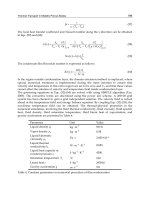
Fig. 13. Unit load carrier

5.1.4 Light load AGV
It can be applied for smaller loads. These are typically used in electronics assembly and
office environments as mail and snack carriers.

5.1.5 Assembly AGV
These are used as assembly platforms, for example car chassis, engines etc., by carrying
products and transport them through assembly stations.

5.1.6 Forklift AGV
It has the ability to pick up and drop off palletized loads both at floor level and on stands.
Generally, these fork lift AGVs have sensors on forks for pallet interfacing.

5.1.7 Rail-Guided Vehicles
These are self-propelled vehicles that ride on a fixed-rail system. These vehicles operate
independently and are driven by electric motors that pick up power from an electrified rail.
Fixed rail system may be:
i. Overhead monorail - suspended overhead from the ceiling
ii. On-floor - parallel fixed rails, tracks generally protrude up from the floor


Fig. 14. Rail guided vehicle
5.2 AGVS System Management
AGVS is a complex system and a number of parameters need to be considered which
include:
Guide-path layout
Number of AGVs required
Operational and transportation control

5.2.1 Guide-path layout
The guide-path layout defines the possible vehicle movement path. Links and nodes that
represent the action points such as pick-up and drop-off points, maintenance areas and
intersections represent the path. The guide-path can be divided into four types:
1. Unidirectional single lane guide-path
2. Bi-directional single lane guide-path
3. Multiple lanes
4. Mixed guide-path.
Generally bidirectional single lane is considered the most cost effective and widely used
layout.

5.2.2 Number of AGVs required
It is important to estimate the optimum number of AGVs required for a system as too many
AGVs will congest the traffic while too few means larger idle time for workstations in a
system. Generally, the number of AGVs required is the sum of the total loaded and empty
travel time and waiting time of the AGVs divided by the time an AGV is available.

5.2.3 Operational and Transportation Control
The operation and transportation consists of vehicle dispatching, vehicle routing and traffic
control issues. Once a demand arises for an AGV, a choice needs to be made regarding the
vehicle to be dispatched among the pool of vehicles available. In an event when several
workstations need servicing, a choice is to be made as to which workstation is to be
serviced. The selection criteria can be applied for assigning the vehicles or workstations
based on one or a combination of the following:
A random vehicle
Longest idle vehicle
Nearest vehicle
Farthest vehicle
Least utilized vehicle

Random workstation
Nearest workstation
Farthest workstation
Maximum queue size
Minimum remaining queue size
First come fist served
Unit load arrival time, due time or priority.
In order to dispatch an AGV to any workstation, it is necessary to find the shortest feasible
path from the existing position. While selecting the shortest path it is necessary to consider
Future Manufacturing Systems134
only those paths which are free and not occupied by vehicles. It may also be necessary to
consider the future positions of the vehicles in the route in addition to their current occupied
positions. In identifying the traffic control systems for AGVs movement, the approaches that
can be used are forward sensing control, zone sensing control and combinatorial control. In
forward sensing control, an AGV is equipped with obstruction detecting sensors that can
identify another AGV in front of it and slow down or stop. This helps in improving the AGV
utilization due to closer allowable distance between vehicles. However, this approach may
not be able to detect the obstacles at intersections and around corners. This is generally
useful for long and straight path which is divided into zones. Once an AGV enters a zone, it
becomes unavailable for other AGVs which may introduce system inefficiency. The main
advantages derived from the use of AGVs in manufacturing environment are:
Dispatching, tracking and monitoring under real time control which help in planned
delivery.
Better resource utilization as AGVs can be economically justified.
Increased control over material flow and movement
Reduced product damage and routing flexibility
Increased throughput because of dependable on-time delivery.

6. Industrial Robots
Industrial robots are very useful material handling devices in an automated environment.

An industrial robot is a reprogrammable multifunctional manipulator designed to move
materials, parts, tools, or other devices by means of variable programmed motions and to
perform a variety of other tasks. It is also defined as a machine formed by a mechanism
including several degrees of freedom often having the appearance of one or several arms
ending in a wrist capable of holding a job, tool and inspection device. It is automatically
controlled, reprogrammable, multipurpose manipulative machine with several
reprogrammable axes which is either fixed in place or mobile for use in industrial
automation applications.

6.1 Robot components
The following are basic components of an industrial robot.

6.1.1 Manipulator
It is a mechanical unit that provides motions similar to those of human arm and hand. The
end of wrist can reach a point in space having a specific set of coordinates in specific
orientation.

6.1.2 End effector
It is attached with the end of wrist in a robot. It is a special purpose tooling which enables
the robot to perform a particular job. Depending on the type of work, end effector may be
equipped with any of the following:
a) Grippers, hooks, vacuum cups, and adhesive fingers for material handling
b) Spray guns for painting
c) Attachments for different kinds of welding processes.
6.1.3 Control system
It is a brain of a robot which gives commands for the movements of the robot. It stores the
data to initiate and terminate movements of the manipulator. It interfaces with the
computers and other equipments such as manufacturing cells or assembly operations.

6.1.4 Power supply

It supplies the power to the controller and manipulator. Each motion of manipulator is
controlled and regulated by actuators that use an electrical, pneumatic or hydraulic power.

6.2 Robot Types
Robots are generally classified as Cartesian or rectilinear, cylindrical, polar or spherical
jointed arms. They are also classified, from material handling point of view, as under:

6.2.1 Pick and place robot
It is also called fixed sequence robot and is programmed for a specific operation. Its
movements are from point to point and cycle is repeated. These robots are simple and
inexpensive and are used to pick and place materials.

6.2.2 Playback robot
This robot learns the work and motions from operator who leads the playback robot and its
end effector through the desired path. The robot memorizes and records the path and
sequence of motions and can repeat them continuously without any further action or
guidance by the operator.

6.2.3 Numerically controlled robot
It is a programmable type of robot and works same as the numerical control machines. The
robot is servo controlled by digital data and its sequence of movements can be changed with
relative ease.

6.2.4 Intelligent robot
It is capable of performing some of the functions and tasks carried out by humans and is
equipped with a variety of sensors with usual and tactile capabilities. It can perform tasks
such as moving among a variety of machines on a shop floor avoiding collisions. It can
recognize, select and properly grip the correct work piece.

6.3 Robot applications in Material handling

The major applications in material handling include:
1. Industrial robots are used to load/ unload materials during operations.
2. These are used to transfer the material from one conveyor to another.
3. These are used in palletizing and de-palletizing in such a way that parts/ materials are
taken from conveyor and are loaded on to a pallet in a desired pattern and sequence
and vice-versa.
4. These are very effective in automated assembly where repetitive work is required.
Materials handling in exible manufacturing systems 135
only those paths which are free and not occupied by vehicles. It may also be necessary to
consider the future positions of the vehicles in the route in addition to their current occupied
positions. In identifying the traffic control systems for AGVs movement, the approaches that
can be used are forward sensing control, zone sensing control and combinatorial control. In
forward sensing control, an AGV is equipped with obstruction detecting sensors that can
identify another AGV in front of it and slow down or stop. This helps in improving the AGV
utilization due to closer allowable distance between vehicles. However, this approach may
not be able to detect the obstacles at intersections and around corners. This is generally
useful for long and straight path which is divided into zones. Once an AGV enters a zone, it
becomes unavailable for other AGVs which may introduce system inefficiency. The main
advantages derived from the use of AGVs in manufacturing environment are:
Dispatching, tracking and monitoring under real time control which help in planned
delivery.
Better resource utilization as AGVs can be economically justified.
Increased control over material flow and movement
Reduced product damage and routing flexibility
Increased throughput because of dependable on-time delivery.

6. Industrial Robots
Industrial robots are very useful material handling devices in an automated environment.
An industrial robot is a reprogrammable multifunctional manipulator designed to move
materials, parts, tools, or other devices by means of variable programmed motions and to

perform a variety of other tasks. It is also defined as a machine formed by a mechanism
including several degrees of freedom often having the appearance of one or several arms
ending in a wrist capable of holding a job, tool and inspection device. It is automatically
controlled, reprogrammable, multipurpose manipulative machine with several
reprogrammable axes which is either fixed in place or mobile for use in industrial
automation applications.

6.1 Robot components
The following are basic components of an industrial robot.

6.1.1 Manipulator
It is a mechanical unit that provides motions similar to those of human arm and hand. The
end of wrist can reach a point in space having a specific set of coordinates in specific
orientation.

6.1.2 End effector
It is attached with the end of wrist in a robot. It is a special purpose tooling which enables
the robot to perform a particular job. Depending on the type of work, end effector may be
equipped with any of the following:
a) Grippers, hooks, vacuum cups, and adhesive fingers for material handling
b) Spray guns for painting
c) Attachments for different kinds of welding processes.
6.1.3 Control system
It is a brain of a robot which gives commands for the movements of the robot. It stores the
data to initiate and terminate movements of the manipulator. It interfaces with the
computers and other equipments such as manufacturing cells or assembly operations.

6.1.4 Power supply
It supplies the power to the controller and manipulator. Each motion of manipulator is
controlled and regulated by actuators that use an electrical, pneumatic or hydraulic power.

6.2 Robot Types
Robots are generally classified as Cartesian or rectilinear, cylindrical, polar or spherical
jointed arms. They are also classified, from material handling point of view, as under:

6.2.1 Pick and place robot
It is also called fixed sequence robot and is programmed for a specific operation. Its
movements are from point to point and cycle is repeated. These robots are simple and
inexpensive and are used to pick and place materials.

6.2.2 Playback robot
This robot learns the work and motions from operator who leads the playback robot and its
end effector through the desired path. The robot memorizes and records the path and
sequence of motions and can repeat them continuously without any further action or
guidance by the operator.

6.2.3 Numerically controlled robot
It is a programmable type of robot and works same as the numerical control machines. The
robot is servo controlled by digital data and its sequence of movements can be changed with
relative ease.

6.2.4 Intelligent robot
It is capable of performing some of the functions and tasks carried out by humans and is
equipped with a variety of sensors with usual and tactile capabilities. It can perform tasks
such as moving among a variety of machines on a shop floor avoiding collisions. It can
recognize, select and properly grip the correct work piece.

6.3 Robot applications in Material handling
The major applications in material handling include:
1. Industrial robots are used to load/ unload materials during operations.

2. These are used to transfer the material from one conveyor to another.
3. These are used in palletizing and de-palletizing in such a way that parts/ materials are
taken from conveyor and are loaded on to a pallet in a desired pattern and sequence
and vice-versa.
4. These are very effective in automated assembly where repetitive work is required.
Future Manufacturing Systems136
5. Intelligent robots can be used to automatically pick the right work piece without
interference of operator and hence improves quality and pace of work.

7. References
M.P. Groover. “Automation, Production systems and computer integrated manufacturing”
Second edition. Pearson-Prentice Hall, 2008.
K. Sareen and C. Grewal.”CAD/CAM: Theory and concepts” S. Chand & Co. 2009.
C. R. Alavala. “ CAD/CAM: Concepts and applications” Prentice-Hall, 2008.
P. N. Rao. “ CAD/CAM: Principles and applications” McGraw-Hill, 2004.
C. R. Asfahl. “Robots and manufacturing automation” Second edition, John-Wiley and
sons.1992.
M. P. Groover and E. W. Zimmers. Jr. “ CAD/CAM: Computer added design and
manufacturing” Pearson-Prentice Hall, 2009.
G. Chryssolouris, “Manufacturing systems: Theory and Practice” Springer-Verlag,1992.
Scheduling methods for hybrid ow shops with setup times 137
Scheduling methods for hybrid ow shops with setup times
Larysa Burtseva, Victor Yaurima and Rainier Romero Parra
X

Scheduling methods for hybrid
flow shops with setup times

Larysa Burtseva
a

, Victor Yaurima
b
and Rainier Romero Parra
c
a
Autonomous University of Baja California, Mexicali,
b
CESUES Superior Studies Center, San Luis Rio Colorado, Sonora,

c
Polytechnic University of Baja California, Mexicali,
Mexico

1. Introduction
Many real manufacturing systems process a large number of product variants in the same
flow. These products may differ in some optional components; consequently, the processing
time on a machine differs from one product to the next, and the need to prepare one or more
machines before beginning or after the finishing of jobs is frequently presented. The
preparation activities are: machine adjustment and feeders preparation to process a next job,
dismantling after a previous job, machine calibrating, inspection of accessories or tools,
cleaning of the machines and adjacent areas, etc. In the scheduling theory, the time required
to shift from one job to another on a given machine is defined as additional production cost
or setup time. The scheduling problems, which consider the setup times, have a high
computational complexity. Pinedo (2008) presents a proof of the NP-hardness of the single
machine case with setup consideration. They are more complex when the resource model
has the parallel machine environment.
The time that a job spends on a machine includes three phases: setup, processing, and
removal. In the majority of investigations dedicated to production planning and scheduling
it is assumed that the setup/removal times are negligible or nonseparable, therefore they are
included in the job processing time, and hence are ignored. The nonseparable setup time

assumption simplifies the analysis, and these problems can be formulated and solved as
standard scheduling problem. However, an explicit treatment of the setup times in most
applications is required and represents a special interest, because machine setup time is a
significant factor for production scheduling in many cases. It may easily consume more than
20% of available machine capacity if it is not well handled (Pinedo, 2008).
Numerous examples of scheduling problems which consider separable setup times are
given in the literature, including electronics manufacturing, automobile assembly plant, the
packaging industry, textile industry, steel manufacturing, airplane engine plant, label sticker
manufacturing company, semiconductor industry, maritime container terminal, ceramic tile
manufacturing sector, as well as in electronics industry in sections for inserting components
on printed circuit boards (PCB), where this kind of problems is frequent.
7
Future Manufacturing Systems138

The purpose of this chapter is to present a class of deterministic scheduling problems in a
multi-stage parallel machine environment called hybrid flow shop with setup times and
appropriate methods for its resolution. The chapter includes a description of model with
necessary definitions and notations; concepts of product family and batch, which are
important elements of setup time analysis as well as a classification of setup times and
problems that each category produces. The last section is focused on problems with
sequence-depended setup times in hybrid flow shops. A review of investigated cases is
explained, including the application of genetic algorithms for this kind of scheduling
problems: structure of a genetic algorithm and description of several crossover operators
appropriated to use based on previous investigations of authors. This section includes an
algorithm and an example of a complex problem solution. A conclusion is presented at the
chapter end.

2. Hybrid flow shop with setup times
In the scheduling theory, a multi-stage production process with the property that all
products have to pass through a number of stages in the same order is classified as a flow

shop. In a simple flow shop, each stage consists of a single machine, which handles at most
one operation at a time. It is more realistic to assume that, at every stage, a number of
machines that operate in parallel are available. This model is known as a hybrid flow shop
(HFS). Some stages may have only one machine, but for the model to be qualified as a HFS,
at least one stage must have multiple machines in parallel. These machines can be identical,
or have different capacities. Each job is processed by at most one machine at each stage. The
flow of products in the plant is unidirectional; each product is processed at only one
machine in each stage.
The HFS models are common in the industry, which have the same technological route for
all products as a sequence of stages, and any stages have a group of machines to realize the
same operation. Various process industries, such as chemical, textile, metallurgical,
semiconductors, printed circuit board, pharmaceutical, oil, food, and automobile
manufacture, can be modeled as a HFS. In such industries, at some stages the facilities are
duplicated in parallel to increase the overall capacities or to balance the capacities of the
stages, or either to eliminate or to reduce the impact of bottleneck stages on the shop floor
capacities.
Among scheduling problems which consider separable setup times in parallel machine
environment, there is a class of problems of a high computational complexity, where setup
from one product to another occurs on a machine; and machine parameters, which have to
be changed during a setup, differ according to the production sequence. It leads to
sequence-dependent setup times and consequently to sequence-dependent setup costs.
A HFS with setup times has the following characteristics:
 There are k stages of processing in a linear order: 1, 2, …, k.
 Each of the n jobs visits the stages in this order, though all jobs do not need to visit all
stages. Stages may be skipped for a particular job, but the process flow for each job is
the same.

 Each stage has a predetermined number of parallel machines. However, the number of
machines varies from stage to stage.
 The processing time for every job on every machine that it visits is known in advance

and is constant.
 A job represents the processing of an item or a set of identical items (a container, a
pallet, a box, a lot or a part) called batch.
 The jobs can belong to different job families. Jobs from the same family may have
different processing times, but they can be processed on a machine after another
without requiring any adjustment of machine in between.
 Every job is to be processed on one machine at a time without preemption and a
machine processes no more than the job at a time. When an operation is started on a
machine, it must be finished without interruption.
 Typically, buffers are located between stages to store intermediate products.
 The problem consists of assigning the jobs to machines at each stage and sequencing
the jobs assigned to the same machine so that some optimality criteria are minimized.
The following index are used to describing the problems: j for job, j = 1,…, n, i for stage,
i = 1, 2, …,k; m
i
for number of machines at the stage i; l for machine index, l = 1, 2, …, m
i
.
The three-field notation

|

|

is used to describe all details of considered HFS problem
variant. The

field denotes the shop configuration, including the shop type and machine
environment per stage. The


field discomposes into four parameter, i.e.

1
,

2
,

3
, and

4
,
positioned as

1

2,
(

3

4
(1)
,

3

4
(2)

, …,

3

4
(


2)
). Here, parameter

1
indicates the considered
shop, and parameter

2
indicates the number of stages. For the HFS notation, FH is in the

1

position, and the value of parameter

2
has to be major that one. For each stage, parameters

3
and

4
indicate the machine set environments. More specifically,


3
indicates information
about the type of the machines while

4
indicates the number of machines in the stage.
The possible machine set environments on the stage i of a HFS are:
1. Single machine (1): a special case; any stages (not all) in a HFS can have only one
machine.
2. Identical machines in parallel (Pm
i
): job j may be processed on any of m
i
machines;
3. Uniformed machines in parallel (Qm
i
): the m
i
machines in the set have different speeds; a
job j may be processed on anyone machine of set, however its processing time is
proportional of the machine speed.
4. Unrelated machines in parallel (Rm
i
): a set of m
i
different machines in parallel. The time
that a job spends on a machine depends on the job and the machine.

When there are several consecutive stages with the same machine set environments, the

parameters

3
and


4
can be grouped as ((

3

4
(i)
)
i=s
k
)
,
where s and k are the index of the first
and the last consecutive stage, respectively. For example, the notation FH4, (1,(P2
(i)
)
i=2
3
,R3
(4)
)
refers to a HFS configuration with four stages where there are one machine at the first stage,
two identical machines in parallel at second and third stages and three unrelated parallel
machines in the fourth stage.

The

field provides the shop properties; also other conditions and details of the processing
characteristics, which may enumerate multiple entries, also may be empty if they are not.
Scheduling methods for hybrid ow shops with setup times 139

The purpose of this chapter is to present a class of deterministic scheduling problems in a
multi-stage parallel machine environment called hybrid flow shop with setup times and
appropriate methods for its resolution. The chapter includes a description of model with
necessary definitions and notations; concepts of product family and batch, which are
important elements of setup time analysis as well as a classification of setup times and
problems that each category produces. The last section is focused on problems with
sequence-depended setup times in hybrid flow shops. A review of investigated cases is
explained, including the application of genetic algorithms for this kind of scheduling
problems: structure of a genetic algorithm and description of several crossover operators
appropriated to use based on previous investigations of authors. This section includes an
algorithm and an example of a complex problem solution. A conclusion is presented at the
chapter end.

2. Hybrid flow shop with setup times
In the scheduling theory, a multi-stage production process with the property that all
products have to pass through a number of stages in the same order is classified as a flow
shop. In a simple flow shop, each stage consists of a single machine, which handles at most
one operation at a time. It is more realistic to assume that, at every stage, a number of
machines that operate in parallel are available. This model is known as a hybrid flow shop
(HFS). Some stages may have only one machine, but for the model to be qualified as a HFS,
at least one stage must have multiple machines in parallel. These machines can be identical,
or have different capacities. Each job is processed by at most one machine at each stage. The
flow of products in the plant is unidirectional; each product is processed at only one
machine in each stage.

The HFS models are common in the industry, which have the same technological route for
all products as a sequence of stages, and any stages have a group of machines to realize the
same operation. Various process industries, such as chemical, textile, metallurgical,
semiconductors, printed circuit board, pharmaceutical, oil, food, and automobile
manufacture, can be modeled as a HFS. In such industries, at some stages the facilities are
duplicated in parallel to increase the overall capacities or to balance the capacities of the
stages, or either to eliminate or to reduce the impact of bottleneck stages on the shop floor
capacities.
Among scheduling problems which consider separable setup times in parallel machine
environment, there is a class of problems of a high computational complexity, where setup
from one product to another occurs on a machine; and machine parameters, which have to
be changed during a setup, differ according to the production sequence. It leads to
sequence-dependent setup times and consequently to sequence-dependent setup costs.
A HFS with setup times has the following characteristics:
 There are k stages of processing in a linear order: 1, 2, …, k.
 Each of the n jobs visits the stages in this order, though all jobs do not need to visit all
stages. Stages may be skipped for a particular job, but the process flow for each job is
the same.

 Each stage has a predetermined number of parallel machines. However, the number of
machines varies from stage to stage.
 The processing time for every job on every machine that it visits is known in advance
and is constant.
 A job represents the processing of an item or a set of identical items (a container, a
pallet, a box, a lot or a part) called batch.
 The jobs can belong to different job families. Jobs from the same family may have
different processing times, but they can be processed on a machine after another
without requiring any adjustment of machine in between.
 Every job is to be processed on one machine at a time without preemption and a
machine processes no more than the job at a time. When an operation is started on a

machine, it must be finished without interruption.
 Typically, buffers are located between stages to store intermediate products.
 The problem consists of assigning the jobs to machines at each stage and sequencing
the jobs assigned to the same machine so that some optimality criteria are minimized.
The following index are used to describing the problems: j for job, j = 1,…, n, i for stage,
i = 1, 2, …,k; m
i
for number of machines at the stage i; l for machine index, l = 1, 2, …, m
i
.
The three-field notation

|

|

is used to describe all details of considered HFS problem
variant. The

field denotes the shop configuration, including the shop type and machine
environment per stage. The

field discomposes into four parameter, i.e.

1
,

2
,


3
, and

4
,
positioned as

1

2,
(

3

4
(1)
,

3

4
(2)
, …,

3

4
(



2)
). Here, parameter

1
indicates the considered
shop, and parameter

2
indicates the number of stages. For the HFS notation, FH is in the

1

position, and the value of parameter

2
has to be major that one. For each stage, parameters

3
and

4
indicate the machine set environments. More specifically,

3
indicates information
about the type of the machines while

4
indicates the number of machines in the stage.
The possible machine set environments on the stage i of a HFS are:

1. Single machine (1): a special case; any stages (not all) in a HFS can have only one
machine.
2. Identical machines in parallel (Pm
i
): job j may be processed on any of m
i
machines;
3. Uniformed machines in parallel (Qm
i
): the m
i
machines in the set have different speeds; a
job j may be processed on anyone machine of set, however its processing time is
proportional of the machine speed.
4. Unrelated machines in parallel (Rm
i
): a set of m
i
different machines in parallel. The time
that a job spends on a machine depends on the job and the machine.

When there are several consecutive stages with the same machine set environments, the
parameters

3
and


4
can be grouped as ((


3

4
(i)
)
i=s
k
)
,
where s and k are the index of the first
and the last consecutive stage, respectively. For example, the notation FH4, (1,(P2
(i)
)
i=2
3
,R3
(4)
)
refers to a HFS configuration with four stages where there are one machine at the first stage,
two identical machines in parallel at second and third stages and three unrelated parallel
machines in the fourth stage.
The

field provides the shop properties; also other conditions and details of the processing
characteristics, which may enumerate multiple entries, also may be empty if they are not.
Future Manufacturing Systems140

The following model properties are frequently associated with a setup time HFS scheduling
problem:

batch(b) Batch processing. A machine is able to process up to b jobs continuously without
any setup.
brkdown Machine breakdown implies that a machine may not be continuously available.
fmls Job families. The n jobs belong to F different job families. Jobs from the same family
may have different processing times, but they can be processed on a machine after
another without requiring any setup in between.
M
jk
Machine eligibility restrictions. Processing of job j is restricted to the set Mj of
machines at stage k.
r
j
Release dates. The job j cannot start processing before release data r
j
.
R Removal time. Machines become free only after the setup of the job has been
removed.
S
si
Sequence-independent setup times. The setup time of machine depends only on the
job to process and does not depend on the previous job.
S
sd
Sequence-dependent setup times. The setup time of machine required to process
next job depends on the previous job.
w
j
The priority factor denoting the weight or importance of job j relative to the other
jobs of system.
The


field establishes the objective to be minimized. The more common objective functions
to minimize in a HFS scheduling problem are:
max
C
as maximum completion time;
max
F
as
maximum flow time;
max
L
as maximum lateness;
max
T
as maximum tardiness;
max
E
maximum earliness, among others. The most used objective function to be minimized
in a HFS scheduling problem is the completion time when the last job to leave the system,
referred to a makespan or C
max
.
A HFS standard scheduling problem with k stages and a number of the identical parallel
machines in each stage is denoted as FHk, ((PM
(i)
)
i=1
k
)||C

max
. In this case, the formula
defines a HFS with k stages, |M
(i)
| identical machines in parallel on stage i, i = 1, …, k; there
are not any special parameter

, and the objective is the makespan minimizing.
Figure 1 illustrates the physical relationship between machines and stages, which
corresponds to the notation FH3, (1, P3
(2)
, R2
(3)
)|M
j3
, S
sd
|T
max
, referring to tri-stage HFS. The
stage 1 has one machine, stage 2 has three identical machines in parallel, and stage 3 has two
parallel unrelated machines; M
j3
and S
sd
indicate that there are machine eligibility
restrictions at stage 3 and setup times depended on the sequence of jobs. The objective is the
maximum tardiness minimizing. Moreover, the figure shows that there are unlimited
buffers between stages to storage unfinished products, so called Work In Process (WIP).
A production system, to be classified as a HFS has to be flexible. It is important to know the

differences between a flexible production system and a traditional one; what exactly means
the concept of flexibility and what justifies the use of specific production planning models
for flexible production systems. Automated manufacturing systems display flexibility in
multiple and intertwined ways, pertaining to the equipment, processes, products,

Input
1
j
n

1
2

3
1
2
Jobs
2
1
Stage 1 Stage 2 Stage 3
End jobs
Buffer
Buffer

Fig. 1. Resource model for a tri-stage HFS.

production volumes, etc. Among the more important concepts, are the following
(Crama, 1997), (Vairaktarakis, 2004):
1. machine flexibility, the ability of the machines to perform various types of operations
without requiring a prohibitive effort in switching from one operation to another;

2. material handling flexibility, the ability of the material handling system to move different
parts efficiently for proper positioning and processing through the manufacturing
facility;
3. operation flexibility, the ability to realize it in different ways;
4. processing flexibility, that means that jobs may skip stages or there is a set of part types
that the system can produce without major setups;
5. routing flexibility, the ability of a manufacturing system to produce a part by alternate
routes through the system.
A planning production model with sets machines in parallel has to comply with one of these
concepts to be classified as a flexible flow shop tacking in account that the flow of products
in the plant is unidirectional. The hybridizing occurs when any products require special
manufacture conditions, e.g., different qualities and capacities of machines at the same
stage, assignment any jobs on certain machines, and another special conditions.
Meanwhile, the HFS has been studied since the 70
th
, the researcher put much attention to
this model and some new designs were discovered on the recent years. This fact probably
implicates confusions in the terminology and notations. Actually, there is not in the
literature a conventional classification of this kind of flow shops. A variety of known models
should be interpreted as a HFS or its special case.
There are:
Flexible flow shop (FFS); a HFS in the parallel identical machine environment when the
machines in each set are identical (processing flexibility within a production stage which is
derived from the ability to process a job on any parallel machine at stage). Some authors, as
e.g., Pinedo (2008), Jungwattanakit et al., (2009) do not use the notion HFS, and describe the
more complex configurations as a FFS with not identical parallel machines at least on one
stage. Moreover, a variety of authors do not differ between terms of FFS and HFS referring
this model as a flexible (hybrid) flow shop (Allahverdi et al., 2008); or use the HFS term in
parallel identical machine environment (Naderi et al., 2009).
Flexible flow line (FFL) and Flow shop with multiple processors (FSMP or MPFS) are equivalent

to a FFS (Lin & Liao, 2003). Zandieh at al. (2006) considering that the HFS is known
commonly as a flexible flow line, because the flow of jobs in that system is unidirectional.
Scheduling methods for hybrid ow shops with setup times 141

The following model properties are frequently associated with a setup time HFS scheduling
problem:
batch(b) Batch processing. A machine is able to process up to b jobs continuously without
any setup.
brkdown Machine breakdown implies that a machine may not be continuously available.
fmls Job families. The n jobs belong to F different job families. Jobs from the same family
may have different processing times, but they can be processed on a machine after
another without requiring any setup in between.
M
jk
Machine eligibility restrictions. Processing of job j is restricted to the set Mj of
machines at stage k.
r
j
Release dates. The job j cannot start processing before release data r
j
.
R Removal time. Machines become free only after the setup of the job has been
removed.
S
si
Sequence-independent setup times. The setup time of machine depends only on the
job to process and does not depend on the previous job.
S
sd
Sequence-dependent setup times. The setup time of machine required to process

next job depends on the previous job.
w
j
The priority factor denoting the weight or importance of job j relative to the other
jobs of system.
The

field establishes the objective to be minimized. The more common objective functions
to minimize in a HFS scheduling problem are:
max
C
as maximum completion time;
max
F
as
maximum flow time;
max
L
as maximum lateness;
max
T
as maximum tardiness;
max
E
maximum earliness, among others. The most used objective function to be minimized
in a HFS scheduling problem is the completion time when the last job to leave the system,
referred to a makespan or C
max
.
A HFS standard scheduling problem with k stages and a number of the identical parallel

machines in each stage is denoted as FHk, ((PM
(i)
)
i=1
k
)||C
max
. In this case, the formula
defines a HFS with k stages, |M
(i)
| identical machines in parallel on stage i, i = 1, …, k; there
are not any special parameter

, and the objective is the makespan minimizing.
Figure 1 illustrates the physical relationship between machines and stages, which
corresponds to the notation FH3, (1, P3
(2)
, R2
(3)
)|M
j3
, S
sd
|T
max
, referring to tri-stage HFS. The
stage 1 has one machine, stage 2 has three identical machines in parallel, and stage 3 has two
parallel unrelated machines; M
j3
and S

sd
indicate that there are machine eligibility
restrictions at stage 3 and setup times depended on the sequence of jobs. The objective is the
maximum tardiness minimizing. Moreover, the figure shows that there are unlimited
buffers between stages to storage unfinished products, so called Work In Process (WIP).
A production system, to be classified as a HFS has to be flexible. It is important to know the
differences between a flexible production system and a traditional one; what exactly means
the concept of flexibility and what justifies the use of specific production planning models
for flexible production systems. Automated manufacturing systems display flexibility in
multiple and intertwined ways, pertaining to the equipment, processes, products,

Input
1
j
n

1
2

3
1
2
Jobs
2
1
Stage 1 Stage 2 Stage 3
End jobs
Buffer
Buffer

Fig. 1. Resource model for a tri-stage HFS.

production volumes, etc. Among the more important concepts, are the following
(Crama, 1997), (Vairaktarakis, 2004):
1. machine flexibility, the ability of the machines to perform various types of operations
without requiring a prohibitive effort in switching from one operation to another;
2. material handling flexibility, the ability of the material handling system to move different
parts efficiently for proper positioning and processing through the manufacturing
facility;
3. operation flexibility, the ability to realize it in different ways;
4. processing flexibility, that means that jobs may skip stages or there is a set of part types
that the system can produce without major setups;
5. routing flexibility, the ability of a manufacturing system to produce a part by alternate
routes through the system.
A planning production model with sets machines in parallel has to comply with one of these
concepts to be classified as a flexible flow shop tacking in account that the flow of products
in the plant is unidirectional. The hybridizing occurs when any products require special
manufacture conditions, e.g., different qualities and capacities of machines at the same
stage, assignment any jobs on certain machines, and another special conditions.
Meanwhile, the HFS has been studied since the 70
th
, the researcher put much attention to
this model and some new designs were discovered on the recent years. This fact probably
implicates confusions in the terminology and notations. Actually, there is not in the
literature a conventional classification of this kind of flow shops. A variety of known models
should be interpreted as a HFS or its special case.
There are:
Flexible flow shop (FFS); a HFS in the parallel identical machine environment when the
machines in each set are identical (processing flexibility within a production stage which is
derived from the ability to process a job on any parallel machine at stage). Some authors, as

e.g., Pinedo (2008), Jungwattanakit et al., (2009) do not use the notion HFS, and describe the
more complex configurations as a FFS with not identical parallel machines at least on one
stage. Moreover, a variety of authors do not differ between terms of FFS and HFS referring
this model as a flexible (hybrid) flow shop (Allahverdi et al., 2008); or use the HFS term in
parallel identical machine environment (Naderi et al., 2009).
Flexible flow line (FFL) and Flow shop with multiple processors (FSMP or MPFS) are equivalent
to a FFS (Lin & Liao, 2003). Zandieh at al. (2006) considering that the HFS is known
commonly as a flexible flow line, because the flow of jobs in that system is unidirectional.
Future Manufacturing Systems142

Hybrid flexible flow shop or Flexible hybrid flow line (HFFL); this model is equivalent to a HFS
where jobs might skip stages (processing flexibility across production stages) (Ruiz &
Vazquez-Rodriguez, 2010), (Allahverdi et al., 2008)
Parallel HFS (PHFS) system represents a HFS decomposed into smaller HFS sub-designs
operated in parallel. More specific, a PHFS is composed of a number of independent sub-
designs each of which is a HFS of the unidirectional routing (routing flexibility)
(Vairaktarakis, 2004).
The HFS scheduling problems which consider setup times are among the most difficult
classes of scheduling problems. It is known, that a one-machine sequence-dependent setup
scheduling problem is equivalent to a traveling-salesman problem which is NP-hard, even
for a small system, the complexity of this problem is beyond the reach of existing theories
(Pinedo, 2008). A HFS restricted to two processing stages, even in the simplest case when
one stage contains two identical machines and the second only a single machine, is already
NP-hard, according to Gupta (1988). Moreover, the special case where there is a single
machine per stage, known as the flow shop, and the simplest case where there is a single
stage with several machines, known as the parallel machine environment, are also NP-hard
(Glover & Laguna., 1997). The total number of possible solutions for a HFS to be n!(П
i=1
k
m

i
)
n
while the number of possible solutions in a regular flow shop scheduling problem is n! The
complicity of a HFS scheduling problem with setup time condition depends essentially on
setup time nature.

3. Batch processing
A technical similarity between products of a plant often reflects an obvious grouping of
them into product groups. Products can be sorted out into groups according to their design
attributes, which include part shape, size, surface texture, material type, raw material estate,
or according to their manufacturing attributes. The technical similarities of the products
within a group permit reduce essentially the setups number on a machine, when a setup
from one product to another occurs and hence manufacturing time would be decreased and
consequently machine usage time would be improved.
This idea is adapted by the Group Technology (GT) (Andrés et al., 2005). The GT concept is
based on the simplification and standardization process. It was dedicated originally to
single machine environment to reduce setup times. This concept was further extended to the
production planning in productive systems which have some available resources in each of
the stages of production and not negligible setups known as the HFS problem with setup
times dependent on the sequence (Li, 1997).
From the GT surge the concepts of product family and batch. The jobs are supposed to be
partitioned into F families, F ≥ 1. A batch is a set of jobs of the same family. Batching occurs
only if setup costs or times are not negligible and several jobs of the same product type have
to be produced. When the processing is realized in batches (lots, pallets, containers, boxes),
the operations processed simultaneously start together and complete together, with just a
single setup in the beginning. Their processing time depends only on the family of the batch.
When one batch is completed, the resources have to be adjusted for the next batch. The time
needed for the setup depends on the families of both adjacent batches. A batch is called

feasible if it can be processed without any tool switches. While families are supposed to be
given in advance, batch formation is a part of the decision making process. To batch-sizes
calculating has to decide how many units must be produced consecutively. In (Liu & Chang,
2000) is indicated that the processing in large batches may increase machine utilization and
reduce the total setup time. However, large batch processing increases the flow time. There
is a tradeoff between flow time and machine utilization by selecting batch size and
scheduling. According to the GT, no family can be split, only a single batch can be formed
for each family.
Batch setup models are further partitioned into batch availability and job availability models.
According to the batch availability model, all the jobs of the same batch become available for
processing and leave the machine together. Two rules that define the processing time of a
batch are distinguished (Lushchakova & Strusevich, 2010):
 In the case of sequential batch processing, also known as ‘‘sum-batch”, the processing
time of a batch on machine is equal to the total processing times of its jobs;
 In the case of simultaneous batch processing, also known as ‘‘max-batch”, the
processing time of a batch on machine is equal to the largest processing time of its jobs.
In the job availability model, each job’s start and completion times are independent on other
jobs in its batch.
The term of family denotes initial job partitioning, while the term of batch is used to denote a
part of the solution. Many publications use the term batch to denote the initial job
partitioning and they use different names like sub-batch, lot, sub-lot, etc., to denote a set of
jobs of the same family processed consecutively on the same machine. In the literature, a job
availability model is considered, if not stated otherwise.
Li (1997) gives an example of scheduling problem from an airplane engine plant, Pratt and
Whitney Inc. (PWI). The blade line, one of the production lines at PWI, characterized as a
two-stages HFS, produces various types of blades used in airplane engines. Each stage of the
blade line at PWI has a different number of machines. The types of blades that have similar
processing requirements are grouped into families. A major setup is required if a machine at
any stage switches from one family of blades to the other. A minor setup is required if a
machine switches from one type of blade to another type in the same family. Since setup

times are not insignificant and unit processing times for all types of blades are very short,
the plant processes each type of blade in batches (lots).
The batch setup time (cost) can be machine dependent or sequence (of families) dependent. It
is sequence-dependent if its duration (cost) depends on the families of both the current and
the immediately preceding batches, and is sequence-independent if its duration (cost)
depends solely on the family of the current batch to be processed.
A HFS scheduling problems with setup times which consider job processing in batches can
be sequence-dependent as well as sequence-independent. Most studies assume that either no
setup has to be performed or that setup times are sequence-independent and there is only a
single unit of each product type. In this case, a job’s setup time may be added to its process
time. However, if setup times are sequence-dependent or if several jobs of the same product
type have to be produced, setups have to be considered explicitly.
Scheduling methods for hybrid ow shops with setup times 143

Hybrid flexible flow shop or Flexible hybrid flow line (HFFL); this model is equivalent to a HFS
where jobs might skip stages (processing flexibility across production stages) (Ruiz &
Vazquez-Rodriguez, 2010), (Allahverdi et al., 2008)
Parallel HFS (PHFS) system represents a HFS decomposed into smaller HFS sub-designs
operated in parallel. More specific, a PHFS is composed of a number of independent sub-
designs each of which is a HFS of the unidirectional routing (routing flexibility)
(Vairaktarakis, 2004).
The HFS scheduling problems which consider setup times are among the most difficult
classes of scheduling problems. It is known, that a one-machine sequence-dependent setup
scheduling problem is equivalent to a traveling-salesman problem which is NP-hard, even
for a small system, the complexity of this problem is beyond the reach of existing theories
(Pinedo, 2008). A HFS restricted to two processing stages, even in the simplest case when
one stage contains two identical machines and the second only a single machine, is already
NP-hard, according to Gupta (1988). Moreover, the special case where there is a single
machine per stage, known as the flow shop, and the simplest case where there is a single
stage with several machines, known as the parallel machine environment, are also NP-hard

(Glover & Laguna., 1997). The total number of possible solutions for a HFS to be n!(П
i=1
k
m
i
)
n
while the number of possible solutions in a regular flow shop scheduling problem is n! The
complicity of a HFS scheduling problem with setup time condition depends essentially on
setup time nature.

3. Batch processing
A technical similarity between products of a plant often reflects an obvious grouping of
them into product groups. Products can be sorted out into groups according to their design
attributes, which include part shape, size, surface texture, material type, raw material estate,
or according to their manufacturing attributes. The technical similarities of the products
within a group permit reduce essentially the setups number on a machine, when a setup
from one product to another occurs and hence manufacturing time would be decreased and
consequently machine usage time would be improved.
This idea is adapted by the Group Technology (GT) (Andrés et al., 2005). The GT concept is
based on the simplification and standardization process. It was dedicated originally to
single machine environment to reduce setup times. This concept was further extended to the
production planning in productive systems which have some available resources in each of
the stages of production and not negligible setups known as the HFS problem with setup
times dependent on the sequence (Li, 1997).
From the GT surge the concepts of product family and batch. The jobs are supposed to be
partitioned into F families, F ≥ 1. A batch is a set of jobs of the same family. Batching occurs
only if setup costs or times are not negligible and several jobs of the same product type have
to be produced. When the processing is realized in batches (lots, pallets, containers, boxes),
the operations processed simultaneously start together and complete together, with just a

single setup in the beginning. Their processing time depends only on the family of the batch.
When one batch is completed, the resources have to be adjusted for the next batch. The time
needed for the setup depends on the families of both adjacent batches. A batch is called

feasible if it can be processed without any tool switches. While families are supposed to be
given in advance, batch formation is a part of the decision making process. To batch-sizes
calculating has to decide how many units must be produced consecutively. In (Liu & Chang,
2000) is indicated that the processing in large batches may increase machine utilization and
reduce the total setup time. However, large batch processing increases the flow time. There
is a tradeoff between flow time and machine utilization by selecting batch size and
scheduling. According to the GT, no family can be split, only a single batch can be formed
for each family.
Batch setup models are further partitioned into batch availability and job availability models.
According to the batch availability model, all the jobs of the same batch become available for
processing and leave the machine together. Two rules that define the processing time of a
batch are distinguished (Lushchakova & Strusevich, 2010):
 In the case of sequential batch processing, also known as ‘‘sum-batch”, the processing
time of a batch on machine is equal to the total processing times of its jobs;
 In the case of simultaneous batch processing, also known as ‘‘max-batch”, the
processing time of a batch on machine is equal to the largest processing time of its jobs.
In the job availability model, each job’s start and completion times are independent on other
jobs in its batch.
The term of family denotes initial job partitioning, while the term of batch is used to denote a
part of the solution. Many publications use the term batch to denote the initial job
partitioning and they use different names like sub-batch, lot, sub-lot, etc., to denote a set of
jobs of the same family processed consecutively on the same machine. In the literature, a job
availability model is considered, if not stated otherwise.
Li (1997) gives an example of scheduling problem from an airplane engine plant, Pratt and
Whitney Inc. (PWI). The blade line, one of the production lines at PWI, characterized as a
two-stages HFS, produces various types of blades used in airplane engines. Each stage of the

blade line at PWI has a different number of machines. The types of blades that have similar
processing requirements are grouped into families. A major setup is required if a machine at
any stage switches from one family of blades to the other. A minor setup is required if a
machine switches from one type of blade to another type in the same family. Since setup
times are not insignificant and unit processing times for all types of blades are very short,
the plant processes each type of blade in batches (lots).
The batch setup time (cost) can be machine dependent or sequence (of families) dependent. It
is sequence-dependent if its duration (cost) depends on the families of both the current and
the immediately preceding batches, and is sequence-independent if its duration (cost)
depends solely on the family of the current batch to be processed.
A HFS scheduling problems with setup times which consider job processing in batches can
be sequence-dependent as well as sequence-independent. Most studies assume that either no
setup has to be performed or that setup times are sequence-independent and there is only a
single unit of each product type. In this case, a job’s setup time may be added to its process
time. However, if setup times are sequence-dependent or if several jobs of the same product
type have to be produced, setups have to be considered explicitly.
Future Manufacturing Systems144

In a non-batch processing environment, a setup time (cost) is incurred prior to the
processing of each job. The corresponding model can also be viewed as a batch setup time
(cost) model in which each family consists of a single job.

4. Classification of HFS with setup times
The setup times, defined as the time required to shift from one job to another on a given
machine, are considered as separable and non-separable from the processing operation.
The non-separable setup times are either included in the processing times or are negligible,
and hence are ignored. There exist some situations in which the nonseparable setup and
removal operations must be modeled and closely coordinated. Such situations are common
in automatic production systems which involve intermediate material handling devices, like
an automatic guided vehicles and robots, loading and unloading (Crama, 1997), (Kim et al.,

1997), (Pinedo, 2008).
When these operations are separable, i.e. they are not a part of processing operation, the
structure of the breakdown time when a job belongs to a machine is as follows (Cheng et al.,
2000):
1) Setup time that is independent on the job sequence. This operation consists of activities
such as fetching the required details, and fixtures, and setting them up on the machine.
2) Setup time that is dependent on the job to be processed. The carrying out of this
operation includes the time required to put the job in the jigs and fixtures and to adjust
the tools.
3) Processing time of the job being processed.
4) Removal time that is independent on the job that has been processed. This operation
includes activities such as dismounting the jigs, the fixtures and/or tools,
inspecting/sharpening of the tools, and cleaning the machine and the adjacent area.
5) Removal time that is dependent on the job that just has been processed. This operation
includes activities such as disengaging the tools from the job, and releasing the job
from the jigs and fixtures.
Three phases of job processing can be grouped as following: the separable setup, the
processing, and the separable removal times represented by items (1, 2), (3), and (4, 5),
respectively. When separable setup/removal times are not negligible in the scheduling
problem, they should be explicitly considered.
The setup times which are separable from the processing times, could be anticipatory
(detached) or non-anticipatory (attached). A setup is anticipatory if it can be started before the
corresponding job or batch becomes available on the machine. In such a situation, the idle
time of a machine can be used to complete the setup of a job on a specific machine.
Otherwise, a setup is non-anticipatory and the setup operations can start only when the job
arrives at a machine as the setup is attached to the job. Further, setup times of a job at a
specific machine could be dependent on the job immediately preceding that job or be
independent on it. If it is not stated explicitly that setups are non-anticipatory.

As follows, a classification of HFS scheduling problems with setup times, derivate from the

classification presented in (Cheng et al., 2000), is described. These problems generally fall
into the following four board categories depending on practical situations (Figure 2):
HFS with ST
Dependent of Independent of
Family sequenceJob sequence
Batch
Group
Batch
Group
Job sequence Family sequence

Fig. 2. Classification of HFS with setup times.

 HFS with sequence-independent job setup times.
 HFS with sequence-dependent job setup times.
 HFS with sequence-independent family setup times:
 HFS with sequence-independent group setup times;
 HFS with sequence-independent batch setup times.
 HFS with sequence-dependent family setup times:
 HFS with sequence-dependent group setup times;
 HFS with sequence-dependent batch setup times.
HFS with sequence-independent job setup times. The setup times are separable from the
processing times and sequence-independent, i.e., depend only on the job to process and do
not depend on the job sequence on this machine. Such setup times could be either detached
or attached to the processing times. However, if this setup time is attached to a job, the idle
time of a machine cannot be used, and hence the setup time have to be considered as a part
of the processing time and the problem can be formulated and solved as a standard HFS
problem. For this reason, only detached sequence-independent job setup times represent a
special interest. Further, removal times could be either zero or positive. The removal times,
if they are present, have to be included in makespan definition.

Three papers with different setup/removal restrictions are mentioned as references. In (Kim
et al., 1997) the C
max
minimizing problem for FFS with two stages, independent setup times
and negligible removal times is considered. A scheduling rule similar to the Johnson's rule is
suggested to minimize makespan. Another work, (Low, 2005), addresses to a HFS with J
stages and unrelated parallel machines at each stage, independent setup and dependent
removal times. The objective is to minimize total flow time in the system. A simulated
annealing-based heuristic is proposed to solve the addressed problem in a reasonable
running time. In (Harjunkoski & Grossmann, 2002) is considered a HFS model where setup
Scheduling methods for hybrid ow shops with setup times 145

In a non-batch processing environment, a setup time (cost) is incurred prior to the
processing of each job. The corresponding model can also be viewed as a batch setup time
(cost) model in which each family consists of a single job.

4. Classification of HFS with setup times
The setup times, defined as the time required to shift from one job to another on a given
machine, are considered as separable and non-separable from the processing operation.
The non-separable setup times are either included in the processing times or are negligible,
and hence are ignored. There exist some situations in which the nonseparable setup and
removal operations must be modeled and closely coordinated. Such situations are common
in automatic production systems which involve intermediate material handling devices, like
an automatic guided vehicles and robots, loading and unloading (Crama, 1997), (Kim et al.,
1997), (Pinedo, 2008).
When these operations are separable, i.e. they are not a part of processing operation, the
structure of the breakdown time when a job belongs to a machine is as follows (Cheng et al.,
2000):
1) Setup time that is independent on the job sequence. This operation consists of activities
such as fetching the required details, and fixtures, and setting them up on the machine.

2) Setup time that is dependent on the job to be processed. The carrying out of this
operation includes the time required to put the job in the jigs and fixtures and to adjust
the tools.
3) Processing time of the job being processed.
4) Removal time that is independent on the job that has been processed. This operation
includes activities such as dismounting the jigs, the fixtures and/or tools,
inspecting/sharpening of the tools, and cleaning the machine and the adjacent area.
5) Removal time that is dependent on the job that just has been processed. This operation
includes activities such as disengaging the tools from the job, and releasing the job
from the jigs and fixtures.
Three phases of job processing can be grouped as following: the separable setup, the
processing, and the separable removal times represented by items (1, 2), (3), and (4, 5),
respectively. When separable setup/removal times are not negligible in the scheduling
problem, they should be explicitly considered.
The setup times which are separable from the processing times, could be anticipatory
(detached) or non-anticipatory (attached). A setup is anticipatory if it can be started before the
corresponding job or batch becomes available on the machine. In such a situation, the idle
time of a machine can be used to complete the setup of a job on a specific machine.
Otherwise, a setup is non-anticipatory and the setup operations can start only when the job
arrives at a machine as the setup is attached to the job. Further, setup times of a job at a
specific machine could be dependent on the job immediately preceding that job or be
independent on it. If it is not stated explicitly that setups are non-anticipatory.

As follows, a classification of HFS scheduling problems with setup times, derivate from the
classification presented in (Cheng et al., 2000), is described. These problems generally fall
into the following four board categories depending on practical situations (Figure 2):
HFS with ST
Dependent of Independent of
Family sequenceJob sequence
Batch

Group
Batch
Group
Job sequence Family sequence

Fig. 2. Classification of HFS with setup times.

 HFS with sequence-independent job setup times.
 HFS with sequence-dependent job setup times.
 HFS with sequence-independent family setup times:
 HFS with sequence-independent group setup times;
 HFS with sequence-independent batch setup times.
 HFS with sequence-dependent family setup times:
 HFS with sequence-dependent group setup times;
 HFS with sequence-dependent batch setup times.
HFS with sequence-independent job setup times. The setup times are separable from the
processing times and sequence-independent, i.e., depend only on the job to process and do
not depend on the job sequence on this machine. Such setup times could be either detached
or attached to the processing times. However, if this setup time is attached to a job, the idle
time of a machine cannot be used, and hence the setup time have to be considered as a part
of the processing time and the problem can be formulated and solved as a standard HFS
problem. For this reason, only detached sequence-independent job setup times represent a
special interest. Further, removal times could be either zero or positive. The removal times,
if they are present, have to be included in makespan definition.
Three papers with different setup/removal restrictions are mentioned as references. In (Kim
et al., 1997) the C
max
minimizing problem for FFS with two stages, independent setup times
and negligible removal times is considered. A scheduling rule similar to the Johnson's rule is
suggested to minimize makespan. Another work, (Low, 2005), addresses to a HFS with J

stages and unrelated parallel machines at each stage, independent setup and dependent
removal times. The objective is to minimize total flow time in the system. A simulated
annealing-based heuristic is proposed to solve the addressed problem in a reasonable
running time. In (Harjunkoski & Grossmann, 2002) is considered a HFS model where setup
Future Manufacturing Systems146

times are included, but they are only dependent on the machine and not on the job. The
objective is to minimize job assignment costs and one-time machine-initialization costs.
HFS with sequence-dependent job setup times (Li, 1997), (Naderi et al., 2009).This situation
occurs when the part of the setup of job i can be used for processing the next job j. It
implicates that the removal time of the job i will depend on the job j to be processed next. On
the other hand, the setup time of job j also depends on the job i being processed currently,
because the setup part of the previous job i can be used for the next job j. The net effect of
these two factors is that the setup time of job j depends on the immediately preceding job i.
Sequence-dependent setup times are of the anticipatory (detached) type because their
nature. Therefore, the setup information cannot move with the job; and sequence-dependent
setup times cannot be of the attached type as information about the currently processed job
i; and the next job j requires to determine the needed setup time to be processed.
HFS with sequence-independent/dependent family setup times. In the above two categories the
setups are associated with individual jobs. However, in many real-world situations, the
processing of jobs is realized taking in account the job family. When jobs belonging to the
same family scheduled contiguously, they only need a common setup operation, and so
called family setup times (FST) are involved. The job partitioning into families implicates two
next situations:
 the setup operation arises only when a machine shifts from processing a job in one
family to processing a job in another family;
 a job containing several identical items may be split into multiple sublots and the setup
operation arises only when a machine shifts from processing the sublot of one job to
processing a sublot of another job.
In general, these FST scheduling problems require two interrelated decisions:

 the size and number of the sublots of each family where the items of a single sublot are
processed together;
 the scheduling of each sublot through the HFS where each sublot requires setup on
each machine. According to the GT assumption, a family does not split into sublots, and
the jobs of the same family are processed together. It refers to so called HFS with group
setup time (GST) problem. However, if the families are split, it requires a solution of an
interrelated batching problem to find the optimal size of each sublot. It refers to a so
called HFS with batch setup times (BST) problems.
Since the BST problems require the solution of two interrelated problems (that of batching
and scheduling), these problems are relatively harder to solve than their corresponding GST
problems requiring only the solution of a scheduling problem (Monma & Potts, 1989).
The setup times in the Sequence-Independent Family Setup Times problem could be either
attached or detached. Since each sublot in case of BST (or family in case of GST problem)
consists of multiple jobs, the sequence-independent setup time cannot be added to the
processing time of any one of these jobs, as the first job in the sequence of the sublot or batch
is not known until the scheduling problem is solved. However, for the sequence-dependent
BST and GST problems, the sequence-dependent sublot or batch setup times are only of the
detached type.

Batch scheduling problem with setup times arises frequently in process industries, parts
manufacturing environments and cellular assembly systems (such as chemical,
pharmaceutical, food processing, metal processing, printing industries and semiconductor
testing facilities). Detailed surveys of the recent publications about HFS with setup times
might be consulted in (Ribas et al., 2010), (Ruiz, 2010), (Allajverdi, et al., 2008), (Zandieh et
al., 2006).

5. HFS with sequence-dependent setup times
5.1 Investigated problems
In recent years, many researchers put attention to the HFS problem with sequence-
dependent setup times in consequence of its complexity, the variety of models as realistic as

theoretical, and used tools to the algorithm creation. On Table 1 are summarized
publications dedicated to the investigation of the HFS with sequence-dependent setup
times. The first column indicates the year of publication, the second is the bibliographical
reference, the third describes the problem; and the final column shows the resolution
method, type of approach as well as other case details.

Year Author Problem Comments
1991 Guinet
( )
1 max
,(( ) )| |{ , }
k
m
k sd
FHm PM S C T


ad-hoc
heuristics,
textile
industry
1993 Adler et al.
( )
1
,(( ) )| |
k
m w
k ad
FMm RM S T


DR, packging
industry
Voss
(1) (2)
max
,(( ,1 )| |
sd
FHm PM S C

TS and
heuristics
1995 Aghezzaf et al.
( )
1 max max
,(( ) )| |{ , , }
k
m
k sd
FHm RM S C F F


MPF,
heuristics,
carpet
manufacturing
1997 Li
(1) (2)
max

2,((1 , ))| , , |
sd
FH PM batch S split C

heuristics,
major and
minor setups,
airplane
engine plant
2000 Liu & Chang
( )
1
,(( ) ))| , |
k
m w w
k sd
FHm PM S block E T



MPF based
heuristics
2003 Kurz & Askin
( )
1 max
,(( ) ))| |
k
m
k sd
FHm PM S C



heuristics
Lin & Liao
( ) (1) (2)
2
1 max
,(( ) ))| , |
k
k sd j
FHm PM S M wT


heuristic, label
sticker
manufacturing
2004 Kurz & Askin
( )
1 max
,(( ) ))| |
k
m
k sd
FHm PM S C


MPF, MPR-
GA
Scheduling methods for hybrid ow shops with setup times 147

times are included, but they are only dependent on the machine and not on the job. The
objective is to minimize job assignment costs and one-time machine-initialization costs.
HFS with sequence-dependent job setup times (Li, 1997), (Naderi et al., 2009).This situation
occurs when the part of the setup of job i can be used for processing the next job j. It
implicates that the removal time of the job i will depend on the job j to be processed next. On
the other hand, the setup time of job j also depends on the job i being processed currently,
because the setup part of the previous job i can be used for the next job j. The net effect of
these two factors is that the setup time of job j depends on the immediately preceding job i.
Sequence-dependent setup times are of the anticipatory (detached) type because their
nature. Therefore, the setup information cannot move with the job; and sequence-dependent
setup times cannot be of the attached type as information about the currently processed job
i; and the next job j requires to determine the needed setup time to be processed.
HFS with sequence-independent/dependent family setup times. In the above two categories the
setups are associated with individual jobs. However, in many real-world situations, the
processing of jobs is realized taking in account the job family. When jobs belonging to the
same family scheduled contiguously, they only need a common setup operation, and so
called family setup times (FST) are involved. The job partitioning into families implicates two
next situations:
 the setup operation arises only when a machine shifts from processing a job in one
family to processing a job in another family;
 a job containing several identical items may be split into multiple sublots and the setup
operation arises only when a machine shifts from processing the sublot of one job to
processing a sublot of another job.
In general, these FST scheduling problems require two interrelated decisions:
 the size and number of the sublots of each family where the items of a single sublot are
processed together;
 the scheduling of each sublot through the HFS where each sublot requires setup on
each machine. According to the GT assumption, a family does not split into sublots, and
the jobs of the same family are processed together. It refers to so called HFS with group
setup time (GST) problem. However, if the families are split, it requires a solution of an

interrelated batching problem to find the optimal size of each sublot. It refers to a so
called HFS with batch setup times (BST) problems.
Since the BST problems require the solution of two interrelated problems (that of batching
and scheduling), these problems are relatively harder to solve than their corresponding GST
problems requiring only the solution of a scheduling problem (Monma & Potts, 1989).
The setup times in the Sequence-Independent Family Setup Times problem could be either
attached or detached. Since each sublot in case of BST (or family in case of GST problem)
consists of multiple jobs, the sequence-independent setup time cannot be added to the
processing time of any one of these jobs, as the first job in the sequence of the sublot or batch
is not known until the scheduling problem is solved. However, for the sequence-dependent
BST and GST problems, the sequence-dependent sublot or batch setup times are only of the
detached type.

Batch scheduling problem with setup times arises frequently in process industries, parts
manufacturing environments and cellular assembly systems (such as chemical,
pharmaceutical, food processing, metal processing, printing industries and semiconductor
testing facilities). Detailed surveys of the recent publications about HFS with setup times
might be consulted in (Ribas et al., 2010), (Ruiz, 2010), (Allajverdi, et al., 2008), (Zandieh et
al., 2006).

5. HFS with sequence-dependent setup times
5.1 Investigated problems
In recent years, many researchers put attention to the HFS problem with sequence-
dependent setup times in consequence of its complexity, the variety of models as realistic as
theoretical, and used tools to the algorithm creation. On Table 1 are summarized
publications dedicated to the investigation of the HFS with sequence-dependent setup
times. The first column indicates the year of publication, the second is the bibliographical
reference, the third describes the problem; and the final column shows the resolution
method, type of approach as well as other case details.

Year Author Problem Comments
1991 Guinet
( )
1 max
,(( ) )| |{ , }
k
m
k sd
FHm PM S C T


ad-hoc
heuristics,
textile
industry
1993 Adler et al.
( )
1
,(( ) )| |
k
m w
k ad
FMm RM S T



DR, packging
industry
Voss
(1) (2)

max
,(( ,1 )| |
sd
FHm PM S C

TS and
heuristics
1995 Aghezzaf et al.
( )
1 max max
,(( ) )| |{ , , }
k
m
k sd
FHm RM S C F F


MPF,
heuristics,
carpet
manufacturing
1997 Li
(1) (2)
max
2,((1 , ))| , , |
sd
FH PM batch S split C

heuristics,
major and

minor setups,
airplane
engine plant
2000 Liu & Chang
( )
1
,(( ) ))| , |
k
m w w
k sd
FHm PM S block E T



MPF based
heuristics
2003 Kurz & Askin
( )
1 max
,(( ) ))| |
k
m
k sd
FHm PM S C


heuristics
Lin & Liao
( ) (1) (2)
2

1 max
,(( ) ))| , |
k
k sd j
FHm PM S M wT


heuristic, label
sticker
manufacturing
2004 Kurz & Askin
( )
1 max
,(( ) ))| |
k
m
k sd
FHm PM S C


MPF, MPR-
GA
Future Manufacturing Systems148

2005 Andres et al.
( )
3
1
3,(( ) ))| |
k

k sd
FH PM S other


MPF, GT
Pearn et al.
( )
1
,(( ) ))| |
k
m
k sd
FHm PM S T


MPF,
heuristics,
packaging
industry
Tang et al.
( )
1 max
,(( ) ))| |
k
m
k sd
FHm PM S C


NN

2006 Ruiz & Maroto
( )
1 max
,(( ) ))| , |
k
m
k sd j
FHm RM S M C


MPR-GA
Zandieh
( )
1 max
,(( ) ))| |
k
m
k sd
FHm PM S C


Artificial
Immune
System
2007 Chen et al.
( )
3
1 max
3,(( ) ))| , , |
k

k sd
FH RM S block prec C


MPF, lower
bounds, TS,
container
terminal
Voss & Witt
( )
1
,(( ) )| |
k
m w
k sd
FHm PM S T


MPF, DR,
heuristics.
Multi-project
RCPSP, steel
manufacturing
2008 Jungwattanakit
et al.
( )
1 max
,(( ) ) (1)| , | )
k
k sd

m
j
FHm RM S r C U
 

 

MPF,
heuristics, GA,
SA, TS
Ruiz et al.
m
( )
1 ax
,(( ) ))| , , , , , |
m
j
k
k sd
FHm RM skip rm lag S M prec C


MPF,
heuristics
2009 Jungwattanakit
et al.
( )
1 max
,(( ) ) (1)| , | )
k

k sd
m
j
FHm RM S r C U
 

 

MPF,
heuristics, DR,
GA
Naderi et al., a
( )
1
,(( ) ))| , |{ , }
k
m
k sd
FHm PM S transport F T


SA
Yaurima et al.
( )
1 max
,(( ) ))| , , |
k
m
k sd j
FHm RM S M buffer C



MPR-GA,
electronic
indusry
Naderi et al., b
( )
1
,(( ) ))| |{ , }
k
m
k sd
FHm PM S F T


SA
Alfieri
( )
1
,(( ) ))| , , |
k
m
k sd
FHm PM S reentry batch several


simulation,
heuristics, TS
Table 1. Investigated problems of HFS with sequence-dependent setup times.

The table shows that in recent years the publications are dedicated to more complex models of
the problem, with unrelated parallel machine environment, release times, limited buffers, lags,
and machine eligibility among others. A general framework to solve the problem includes:
dispatching rules (DR), neural networks (NN), tabu search (TS), multiple permutation
representation (MPR), local search (LS), simulated annealing (SA), genetic algorithms (GA).
Mathematical programming formulation (MPF) is developed for many models.
The procedures to seek a solution of a HFS problem can be classified into two principal
categories (Quadt & Kuhn, 2007): optimal procedures and heuristics. The literature does not

report application of any optimal procedure, like Dynamic Programming or Branch &
Bound methods, to solution of a HFS problem with sequence-dependent setup times.
Heuristics do not necessarily find an optimal solution. However, they are usually faster than
optimal procedures and some of them are used for realistic problem sizes. Heuristics may be
split into holistic and decomposition approaches. Holistic approaches consider the complete
scheduling problem in an integrated way. A simple holistic approach is to use dispatching
rules to select the next job that has to be produced whenever a machine becomes idle. The
use of such heuristics is very common in HFS, see, e.g., (Adler et al., 1993), (Voss & Witt,
2007), (Jungwattanakit et al., 2009).
Most holistic procedures are local search methods or metaheuristics. In HFS, a job consists of
several operations, one for each production stage. Thus, a HFS schedule assigns machine for
each operation as well as a production sequence for each machine. A move to a neighboring
schedule may change the machine assignment of an operation or its position in the
sequence. This neighborhood is very large. Hence, local search procedures and
metaheuristics must find ways to limit the size of the neighborhood. This can be done by
only allowing certain moves that appear promising. Examples of metaheuristic techniques
application are given in (Tang et al., 2005), (Chen et al., 2007), (Naderi et al., 2009), (Yaurima
et al., 2009), among others.
In contrast to holistic approaches, decomposition approaches divide the problem into
segments that are considered consecutively, with respect to the production stages, the
individual jobs, or the sub-problems to be solved (batching, loading, and sequencing), e.g.,

(Li, 1997), (Alfieri, 2009).
The HFS scheduling problems with sequence-dependent setup times are among the most
difficult classes of scheduling problems. When a practical problem of large instance sizes
does not require of a fast result obtain, a good approximate solutions are achieved through a
genetic algorithm (GA).

5.2 GA approach
A GA is a well known search technique used to find solutions to optimization problems. It
was proposed by Holland (1975). All GA act according to the scheme represented on Figure
3. Candidate solutions are encoded by chromosomes (also called genomes or individuals).
The set of initial individuals forms the population. Fitness values are defined over the
individuals and measure the quality of the represented solution. The genomes are evolved
through the genetic operators generation by generation to find optimal or near-optimal
solutions. Three genetic operators are repeatedly applied: selection, crossover, and
mutation. The selection picks chromosomes to mate and produce offspring. The crossover
combines two selected chromosomes to create next generation of chromosomes. The
mutation randomly reorganizes the structure of genes in a chromosome, so that a new
combination of genes may appear in the next generation. The individuals evolve until some
stopping criterion is met.
The first paper was by Ruiz and Maroto (2006) where application of GA techniques to HFS
problem with sequence-dependent setup times had been realized. There were considered
the makespan minimization criterion on a m-stage problem with unrelated parallel
machines, sequence-dependent setup times and machine eligibility. The proposed GA was
Scheduling methods for hybrid ow shops with setup times 149

2005 Andres et al.
( )
3
1
3,(( ) ))| |

k
k sd
FH PM S other


MPF, GT
Pearn et al.
( )
1
,(( ) ))| |
k
m
k sd
FHm PM S T


MPF,
heuristics,
packaging
industry
Tang et al.
( )
1 max
,(( ) ))| |
k
m
k sd
FHm PM S C


NN
2006 Ruiz & Maroto
( )
1 max
,(( ) ))| , |
k
m
k sd j
FHm RM S M C


MPR-GA
Zandieh
( )
1 max
,(( ) ))| |
k
m
k sd
FHm PM S C


Artificial
Immune
System
2007 Chen et al.
( )
3
1 max
3,(( ) ))| , , |

k
k sd
FH RM S block prec C


MPF, lower
bounds, TS,
container
terminal
Voss & Witt
( )
1
,(( ) )| |
k
m w
k sd
FHm PM S T


MPF, DR,
heuristics.
Multi-project
RCPSP, steel
manufacturing
2008 Jungwattanakit
et al.
( )
1 max
,(( ) ) (1)| , | )
k

k sd
m
j
FHm RM S r C U
 

 

MPF,
heuristics, GA,
SA, TS
Ruiz et al.
m
( )
1 ax
,(( ) ))| , , , , , |
m
j
k
k sd
FHm RM skip rm lag S M prec C


MPF,
heuristics
2009 Jungwattanakit
et al.
( )
1 max
,(( ) ) (1)| , | )

k
k sd
m
j
FHm RM S r C U
 

 

MPF,
heuristics, DR,
GA
Naderi et al., a
( )
1
,(( ) ))| , |{ , }
k
m
k sd
FHm PM S transport F T


SA
Yaurima et al.
( )
1 max
,(( ) ))| , , |
k
m
k sd j

FHm RM S M buffer C


MPR-GA,
electronic
indusry
Naderi et al., b
( )
1
,(( ) ))| |{ , }
k
m
k sd
FHm PM S F T


SA
Alfieri
( )
1
,(( ) ))| , , |
k
m
k sd
FHm PM S reentry batch several


simulation,
heuristics, TS
Table 1. Investigated problems of HFS with sequence-dependent setup times.

The table shows that in recent years the publications are dedicated to more complex models of
the problem, with unrelated parallel machine environment, release times, limited buffers, lags,
and machine eligibility among others. A general framework to solve the problem includes:
dispatching rules (DR), neural networks (NN), tabu search (TS), multiple permutation
representation (MPR), local search (LS), simulated annealing (SA), genetic algorithms (GA).
Mathematical programming formulation (MPF) is developed for many models.
The procedures to seek a solution of a HFS problem can be classified into two principal
categories (Quadt & Kuhn, 2007): optimal procedures and heuristics. The literature does not

report application of any optimal procedure, like Dynamic Programming or Branch &
Bound methods, to solution of a HFS problem with sequence-dependent setup times.
Heuristics do not necessarily find an optimal solution. However, they are usually faster than
optimal procedures and some of them are used for realistic problem sizes. Heuristics may be
split into holistic and decomposition approaches. Holistic approaches consider the complete
scheduling problem in an integrated way. A simple holistic approach is to use dispatching
rules to select the next job that has to be produced whenever a machine becomes idle. The
use of such heuristics is very common in HFS, see, e.g., (Adler et al., 1993), (Voss & Witt,
2007), (Jungwattanakit et al., 2009).
Most holistic procedures are local search methods or metaheuristics. In HFS, a job consists of
several operations, one for each production stage. Thus, a HFS schedule assigns machine for
each operation as well as a production sequence for each machine. A move to a neighboring
schedule may change the machine assignment of an operation or its position in the
sequence. This neighborhood is very large. Hence, local search procedures and
metaheuristics must find ways to limit the size of the neighborhood. This can be done by
only allowing certain moves that appear promising. Examples of metaheuristic techniques
application are given in (Tang et al., 2005), (Chen et al., 2007), (Naderi et al., 2009), (Yaurima
et al., 2009), among others.
In contrast to holistic approaches, decomposition approaches divide the problem into
segments that are considered consecutively, with respect to the production stages, the

individual jobs, or the sub-problems to be solved (batching, loading, and sequencing), e.g.,
(Li, 1997), (Alfieri, 2009).
The HFS scheduling problems with sequence-dependent setup times are among the most
difficult classes of scheduling problems. When a practical problem of large instance sizes
does not require of a fast result obtain, a good approximate solutions are achieved through a
genetic algorithm (GA).

5.2 GA approach
A GA is a well known search technique used to find solutions to optimization problems. It
was proposed by Holland (1975). All GA act according to the scheme represented on Figure
3. Candidate solutions are encoded by chromosomes (also called genomes or individuals).
The set of initial individuals forms the population. Fitness values are defined over the
individuals and measure the quality of the represented solution. The genomes are evolved
through the genetic operators generation by generation to find optimal or near-optimal
solutions. Three genetic operators are repeatedly applied: selection, crossover, and
mutation. The selection picks chromosomes to mate and produce offspring. The crossover
combines two selected chromosomes to create next generation of chromosomes. The
mutation randomly reorganizes the structure of genes in a chromosome, so that a new
combination of genes may appear in the next generation. The individuals evolve until some
stopping criterion is met.
The first paper was by Ruiz and Maroto (2006) where application of GA techniques to HFS
problem with sequence-dependent setup times had been realized. There were considered
the makespan minimization criterion on a m-stage problem with unrelated parallel
machines, sequence-dependent setup times and machine eligibility. The proposed GA was
Future Manufacturing Systems150

superior to
STOPPING
CRITERION
INPUT

CROSSOVER
MUTATION
OUTPUT
POPULATION
EVALUATION
SELECTION

Fig. 3. GA scheme

a wide range of heuristics and other metaheuristics, among them, ACO based heuristics, TS
procedures, other GAs, SA and deterministic procedures. A similar problem, with unrelated
parallel machines at each stage, and setup times, was approached in (Jungwattanakit, et al.
2008) using GAs and later in (Jungwattanakit, et al., 2009) applying several heuristics
including DR, GA, tailored heuristics, TS and SA. In these two papers, the authors study a
linear combination of the makespan and a number of tardy jobs as an objective. Recently, in
(Yaurima, et al., 2009) is proposed a GA for a complex HFS problem considering makespan
minimization on an m-stage problem with sequence-dependent setup times, unrelated
parallel machines, machine eligibility and limited buffers.

5.3 Crossover operators
The crossover operator is an important factor for a good performance of the GA. The
following crossover operators should be considered to solve the examined problem
according to previous investigations of authors.
1. OBX - Order Based Crossover (Gen, 1997), (Figure 4).


Fig. 4. OBX Crossover

This operator is based on a binary mask. The values of the mask equal to one indicate that
the corresponding sequence of elements from parent 1 to child, is copied. The remaining

7

1

9

8

4

6 2

5 3
1

2
3
4

5
6
7

8 9
7

2
3

1

5

4 6

8
9
1

2
3
4

5
6
7

8 9
Father 2

0
1

1 0

1 0

0
1

1

1 2

3

4
5
6
7
8

9
Mask

1
2
3

4
5

6

7

8
9

1

2 3 4
5
6
7

8 9

Father 1

Child


elements from parent 2 are copied. The mask values are generated randomly and uniformly
in all crossover operations.
2. PPX - Precedence Preservative Crossover (Bierwirth, et al., 1996), (Figure 5).


Fig. 5. PPX Crossover

This operator is based on a binary mask. The values of the mask equal to 1 indicate that
corresponding elements from parent 1 are copied to child and values equal to 0 indicates that the
elements are copied from parent 2, according to each value of the mask one at a time alternately.
3. OSX - One Segment Crossover (Guinet & Salomon, 1996), (Figure 6).


Fig. 6. OSX Crossover

Two points are randomly chosen. The elements from parent 1 since position 1 to the first
place are copied. Elements from parent 2 since first point to the second point are copied.
Finally, the items from parent 1 since the second point to last position are copied,

considering not copied elements.
4. TP - Two Point (Michalewicz, 1996), (Figure 7).
5
4 6

3

1

9 2

7
8

1 2 3

4

5
6

7

8

9

1
2
3

4 5

6
9

7

8

1 2
3

4

5 6

7

8

9

Father 2

1

2 3 4 5

6

7

8

9

1 2
3

4

5

6

7

8
9

Father 1

Child

Point 1

Point 2
7

1

9 8 4

6 2
5
3
1

2
3

4

5

6
7
8

9

7

1
2
9
3

8

4

5 6

1

2
3

4

5

6
7
8

9

Father 2

0

1

1

0

1 0

0

1 1
1 2

3
4
5
6

7

8

9
Mask

1
2
3

4
5

6
7
8

9

1

2 3

4
5
6

7
8 9

Father 1

Child

Scheduling methods for hybrid ow shops with setup times 151

superior to
STOPPING
CRITERION
INPUT
CROSSOVER
MUTATION
OUTPUT
POPULATION
EVALUATION
SELECTION

Fig. 3. GA scheme

a wide range of heuristics and other metaheuristics, among them, ACO based heuristics, TS
procedures, other GAs, SA and deterministic procedures. A similar problem, with unrelated
parallel machines at each stage, and setup times, was approached in (Jungwattanakit, et al.
2008) using GAs and later in (Jungwattanakit, et al., 2009) applying several heuristics
including DR, GA, tailored heuristics, TS and SA. In these two papers, the authors study a
linear combination of the makespan and a number of tardy jobs as an objective. Recently, in
(Yaurima, et al., 2009) is proposed a GA for a complex HFS problem considering makespan
minimization on an m-stage problem with sequence-dependent setup times, unrelated
parallel machines, machine eligibility and limited buffers.

5.3 Crossover operators
The crossover operator is an important factor for a good performance of the GA. The
following crossover operators should be considered to solve the examined problem
according to previous investigations of authors.
1. OBX - Order Based Crossover (Gen, 1997), (Figure 4).


Fig. 4. OBX Crossover

This operator is based on a binary mask. The values of the mask equal to one indicate that
the corresponding sequence of elements from parent 1 to child, is copied. The remaining
7

1

9

8

4

6 2

5 3
1

2
3
4

5
6
7

8 9
7

2
3

1
5

4 6

8
9
1

2

3
4

5
6
7

8 9
Father 2

0
1

1 0

1 0

0
1

1

1 2

3

4
5
6
7

8

9
Mask

1
2
3

4
5

6

7

8
9

1

2 3 4
5
6
7

8 9

Father 1

Child


elements from parent 2 are copied. The mask values are generated randomly and uniformly
in all crossover operations.
2. PPX - Precedence Preservative Crossover (Bierwirth, et al., 1996), (Figure 5).


Fig. 5. PPX Crossover

This operator is based on a binary mask. The values of the mask equal to 1 indicate that
corresponding elements from parent 1 are copied to child and values equal to 0 indicates that the
elements are copied from parent 2, according to each value of the mask one at a time alternately.
3. OSX - One Segment Crossover (Guinet & Salomon, 1996), (Figure 6).


Fig. 6. OSX Crossover

Two points are randomly chosen. The elements from parent 1 since position 1 to the first
place are copied. Elements from parent 2 since first point to the second point are copied.
Finally, the items from parent 1 since the second point to last position are copied,
considering not copied elements.
4. TP - Two Point (Michalewicz, 1996), (Figure 7).
5
4 6

3

1

9 2

7
8

1 2 3

4

5
6

7

8

9

1
2
3

4 5

6
9

7

8

1 2
3

4

5 6

7

8

9

Father 2

1

2 3 4 5

6

7

8

9

1 2
3

4

5

6

7

8
9

Father 1

Child
Point 1

Point 2
7

1

9 8 4

6 2
5
3
1

2

3

4

5

6
7
8

9

7

1
2
9
3

8
4

5 6

1

2
3

4

5

6
7
8

9

Father 2

0

1

1

0

1 0
0

1 1
1 2

3
4
5
6

7

8

9
Mask

1
2
3

4
5

6
7
8

9

1

2 3

4
5
6

7
8 9

Father 1

Child

Future Manufacturing Systems152

Two points are randomly chosen. The elements from parent 1 since first position to the first
point and since second point to the last position are copied. The elements from parent 2
since first point to the second point are copied.

Fig. 7. TP Crossover

5. SB2OX - Similar Block 2-Point Order Crossover (Ruiz & Maroto, 2006), (Figure 8).
The common blocks in both parents (at least two consecutive identical jobs) are copied to the
children, then two random cut points are defined and the section between these two points
directly copied to children. The missing elements of each offspring are copied in the relative
order of the other parent.
6. ST2PX - Setup Time Two Point Crossover (Yaurima, et al., 2009), (Figure 9).
In this crossover operator the sequence-dependent setup time is considered. Two points
randomly in the sequence are chosen. The elements since first position to the first point and
since second point to the last position, are copied from parent 1. The elements since first
point to the second point are copied from parent 2 according to the minimum setup time of
one machine randomly chosen from the first stage.

5.4 A problem of makespan minimizing in a HFS with multiple constrains
A complex problem of makespan minimizing in a HFS with sequence-dependent setup
times, unrelated machines, availability constraints and limited buffers is presented. The real
case of the television production environment is considered (Yaurima, et al., 2009).
Different television models are distinguished by their set of PCBs. The monthly production

plan is developed based on current requirements, machines availability and resource
constrains. It is updated daily depending on the final section requirements. It is examined the
auto-Insertion section, where various PCB types are manufactured with automated machines
for 70 television models, 45 machines and production units of different brands are dealt with.
The auto-insertion section is represented by a HFS with six stages (operations) common for
all PCB types. However, some PCBs do not require all six operations. Each stage consists of
several insertion machines in parallel, and they are dedicated to the certain types of
component processing. At each instant of time, each machine works on at most one PCB,
4 1

8

3

6
9

2

5

7
1

2

3 4
5

6

7

8 9
1
2

3

4
6

5

7

8

9
1

2

3
4
5

6 7

8 9
Father 2

1
2

3

4

5 6
7

8
9
1

2

3 4

5
6

7

8

9

Father 1

Child
Point 1

Point 2

and each PCB is processed by at most one machine. The PCBs are moving along the
assembly line, from one machine to another until it became a complete unit.


a)

b)

c)
Fig. 8. SB2OX Crossover:
a) the common jobs in both parents are copied over to the offspring;
b) jobs before a randomly chosen cut point are inherited from the direct parent;
c) the missing elements in the offspring are copied in the relative order of the other parent.
The flow is determined by technological constraints. Machines of different brands with
identical functionality but with different speeds or capabilities are included in the stage. The
processing time depends on the machine brand. It is considered scheduling in the presence
of machine eligibility restrictions when not all machines can process all PCBs, and machine
availability restrictions when the use of machines depends on their current state: active or in
maintenance service. Adjustment of the machine and the preparation of its feeder are
required when the board type is changed. The feeders have different capacities (number of
slots). For example, machines could have 60 slots or 80 slots. The time needed for
adjustment essentially depends on the board type previously processed in the machine. It
cannot be neglected in the television PCB production environment. Hence, a sequence-
dependent setup time is needed. Each machine has a limited capacity buffer for storing WIP.
If the storage is filled to full capacity, the production on this machine is blocked.

The problem is modeled as a HFS with the following constraints: (1) From two to six
successive stages with the common flow pattern for all PCB types; (2) Stages with unrelated
machines; (3) Machine eligibility/availability; (4) Sequence-dependent setup time; (5)
Limited buffers. The goal is to find a schedule that minimizes the total production time.
3

3

8

8

19
9

9

7

7

6

14

14

17

17

5

15

15

1

1

11

11

16

16

18

19

4

6

2

18

10

10

20

5

13

13

12

4

2

20

12

Father 2

3
3

19

19

8

6

6

7

9

9

5

5

17

15

15

1

1

8

14

14

4

2

7

16

13

13
12

Father 1

4

2

12

Child 1

Child 2

3

8

8

9

7

7

14

1
7
1
7
15
1

1

11

16
16
19
4

6

2

18 10

20
5

13

12

4

2

20
12
Father 2
3

19

19

6

6

9

5

5

15

1

1

8

14 4

2

7

16

13
12
Father 1
4

2

12
Child 1

Cut point 1
Cut point 1
Cut point 2

Cut point 2
Child 2

3

8

9

7

14 1
7
15 1

11 16

19

4

6

2

18

10 20
5

13

12
4

2

20
12
Child 2

3

19 6

9

5

15
1

8

14

4

2

7

1613
12
Father 1
4

2

12
Child 1

Child 2