Process Management Part 3 potx
Bạn đang xem bản rút gọn của tài liệu. Xem và tải ngay bản đầy đủ của tài liệu tại đây (3.63 MB, 25 trang )
A Design for Quality Management Information System in Short Delivery Time Processes
37
40 50 60 70 80 90 100 110 120
0.05 1176.9 1302.2 1377.4 1422.1 1448.7 1464.6 1474.0 1479.5 1482.7
0.10 1090.8 1135.5 1155.3 1163.8 1167.3 1168.6 1169.05 1169.06 1168.9
0.15 1017.8 1023.5 1024.6 1024.8 1024.6 1024.4 1024.15 1023.88 1023.6
0.20 961.3 949.7 944.8 942.8 941.9 941.4 941.03 940.71 940.4
0.30 890.0 863.6 855.2 852.0 850.6 849.9 849.47 849.11 848.8
0.35 860.0 836.8 827.7 824.2 822.8 822.0 821.58 821.21 820.9
0.40 840.0 816.2 806.6 802.9 801.4 800.6 800.12 799.74 799.4
0.46 824.1 796.0 786.0 782.1 780.5 779.7 779.25 778.87 778.5
0.50 810.0 786.4 776.1 772.2 770.5 769.7 769.25 768.87 768.5
0.55 800.0 775.2 764.8 760.8 759.1 758.3 757.79 757.40 757.1
0.60 799.0 765.9 755.2 751.1 749.5 748.6 748.13 747.74 747.4
0.65 791.0 757.9 747.1 742.9 741.2 740.4 739.88 739.49 739.1
0.70 781.4 751.0 740.0 735.8 734.1 733.3 732.76 732.37 732.0
0.75 775.7 744.9 733.9 729.7 727.9 727.1 726.55 726.15 725.8
0.80 770.6 739.6 728.5 724.2 722.4 721.6 721.08 720.68 720.3
0.85 766.2 734.9 723.7 719.4 717.6 716.7 716.23 715.83 715.5
0.90 762.1 730.7 719.4 715.1 713.3 712.4 711.90 711.50 711.1
0.95 758.5 726.9 715.5 711.2 709.4 708.5 708.01 707.61 707.3
1.00 755.3 723.5 712.0 707.7 705.9 705.0 704.50 704.10 703.7
Pa
T
Table 2. The balance of Pa, T and Ct
From Tables 2, it also can be understood that how much total expectation cost should be
paid by the different power, when the delivery time is strictly demanded; how much total
expectation cost should be paid by different delivery time, when the power of process is
strictly demanded. Because Table 2 shows the relation (concrete value) of power, the
delivery date and the total expectation cost, it would become a reference for business plan.
D. The balance of k, T and Ct
In this section, we study the relations between the delivery time and ACT time and the total
expectation cost, then we investigate the balance of control limits width (k) and delivery
time (T) and the total expectation cost (Ct) by numerically analyzing the above design.
Where, c
0
=1
,
c
1
=0.1
,
c
2
=10, c
3
=50, c
4
=25,
a
c
β
=
p
c
β
=
d
c
β
=200,
c
c
β
=2400, n
1
=4, v
1
=0.0316,
Tp=1,
1
φ
=0.01,
2
φ
=0.001, λ
1
=1.
Table 3 show the balance of the quality (control limits width) and delivery time and the total
expectation cost of the above case, which is useful for setting the optimal delivery time and
control limits width to the supplier.
Process Management
38
Table 3. The balance of
k, T and Ct
A Design for Quality Management Information System in Short Delivery Time Processes
39
From Table 3, it can be understood that this tables are divided into two areas by the changed
control limits width: in the colorlessness area, the expected total cost per unit time
(Ct)
increases with the increase of delivery time
(T); in the blue area, the expected total cost per
unit time
(Ct) decreases with the increase of delivery time (T).
From Table 3 and Figure 5, it can be noted that the expected total cost per unit time
(Ct)
increases with the increase of control limits width
(k). This is because that the cost of
defective goods increases by the increase of control limits width.
Fig. 5. The relation between
k and Ct (T=2, T=5).
Fig. 6. The relation between
T, k and Ct.
From Table 3, it also can be understand that a longer delivery time should be set when the
high quality (when
k is small) is demanded, while a shorter delivery time should be set
when the low quality is demanded from an economic aspect.
In addition, to clarify it more, we also show the Figure 6 which is the same as the case of
Table 3.
Ct(T=2)>Ct(T=5) Ct(T=2)<Ct(T=5)
Process Management
40
Table 4. The balance of
a, T and Ct
A Design for Quality Management Information System in Short Delivery Time Processes
41
E. The relation between T, a and Ct
Fig. 7. The relation between
a and Ct (T=2, T=10)
Fig. 8. The relation between
T, a and Ct
Figure 7 show the relation between the delivery time and ACT time and the total expectation
cost, which is useful for setting the optimal delivery time and ACT time to the supplier.
From Figure 7, it can be understood that this tables are divided into two areas by the
changed ACT time: in the colorlessness area, the expected total cost per unit time
(Ct)
increases with the increase of delivery time
(T); in the blue area, the expected total cost per
unit time
(Ct) decreases with the increase of delivery time (T).
From Figure 7 and Table 5, it can be noted that the expected total cost per unit time
(Ct)
increases with the increase of Act time
(a). This is because that the cost of defective goods
increases by the increase of ACT time. Also it can be understand that a longer delivery time
should be set when the ACT time is long, while a shorter delivery time should be set when
the ACT time is short from an economic aspect.
In addition, to clarify it more, we also show the Figure 8 which is the same as the case of
Figure 7.
Ct(T=2)>Ct(T=10)
Ct(T=2)<Ct(T=10)
Process Management
42
4. Conclusions
In this research, from an economic viewpoint, a design of the x control chart is analyzed for
quality management information system used in short delivery time processes.
Because of competition in markets, studying the balance of quality and the delivery time
and cost has become a new problem to manager. To resolve this problem, the mathematical
formulations which correspond to this design were shown, and then by numerically
consideration using the data from real situation, the relations of the power of process and
delivery time and the total expectation cost, the balance of quality (control limits width) and
delivery time and the total expectation cost, the relations between the delivery time, ACT
time and the total expectation cost are discussed, respectively. Moreover, the presented
design based on the judgment rules of JIS Z 9021 was studied.
Some comments are drawn as follows, which would become useful references for setting the
optimal delivery time, ACT time and the power of process to manager.
1.
The expected total cost per unit time decreases with the increase of the power of process.
2.
The power by the two rules (3σ rule and 9 ARL rule) increases with the increase of
sample size
n, and the speed of increase of 9 ARL rule is faster.
3.
A longer delivery time should be set when the higher power for higher quality is
demanded from an economic aspect.
4.
A longer delivery time should be set when the ACT time is long, from an economic aspect.
5. References
[1] K. Amasaka, ed., “Manufacturing Fundamentals: The Application of Intelligence Control
Chart- Digital Engineering for Superior Quality Assurance”
, Japanese Standards
Association , 2003 (in Japanese).
[2] Y. Kanuma, and Y. Suzuki, and T. Kamagata, “Application and Efficiency of FDAS for
Strengthening Real Working Front Ability”,
Proceedings on the 37st Research
Conference of Japanese Society for Quality Control
, pp.161-164, 2007 (in Japanese).
[3] Y. Ando, “An activity report of ‘control chart practical applications study group’ in
JSQC”,
Proceedings on the 5th ANQ Quality Congress, 2007.
[4] S. Yasui, “On key factors for effective process control based on control charts through
investigating literature cases”,
Proceedings on the 37st Research Conference of Japanese
Society for Quality Control
, pp.169-172, 2007 (in Japanese).
[5] J. Sun, M. Tsubaki and M. Matsui, “The comparisons between two quality control cycles-when
the time of in-control and time of out-of-control is independent”,
Proceedings on the 31st
Research Conference of Japanese Society for Quality Control
, pp.227-230, 2003 (in Japanese).
[6] J. Sun, M. Tsubaki and M. Matsui, “Economic considerations in CAPD Model of P
Control Chart for Quality Improvement”,
International Conference on Quality ’05-
Tokyo Proceedings
, pp.VI-10, 2005.
[7] J. Sun, M. Tsubaki and M. Matsui, “Economic Models of
x Chart with Tardiness Penalty
in Finite Due Time Processes,”
Journal of Japan Industrial management Association, (in
Japanese), vol. 57, no.5, pp.374-387, 2006.
[8] Japanese Industrial Standards Committee (1998): “
JIS Z 9021: The Shewhart Control Chart”,
Japanese Standards Association (in Japanese).
[9] Y. Katou, “Verification of judgment rules of Shewhart control chart (JIS Z 9021)”,
Proceedings on the 37st Research Conference of Japanese Society for Quality Control,
pp.165-168, 2007 (in Japanese).
[10] S. P. Ladany and D. N.Bedi, “Selection of the Optimal Setup Policy,”
Naval research
Logistics Quarterly
, vol. 23, pp.219-233, 1976.
4
Design Cycle Period Management
Bahram Soltanmohammad
Sharif University of Technology
IRAN
1. Introduction
As competition increases and new technologies emerge, the civil aerospace industries need
relatively better appropriate frameworks to guarantee their success. Efficient and close
interactions among all disciplines involved in the aircraft design process from
manufacturing, to the flight testing, are essential for improving the quality of the product.
However, such necessities generally lead to a lengthy design cycle. Because of this, a
strategy for cycle time reduction (CTR) must always be available. This process is called
Integrated Airframe Design (IAD), (AGARD Report 814). A proper CTR leads to lessened
costs which is essential in surviving a competition since time, cost and quality are three
parameters that are normally used to evaluate the efficiency of a design process (Ullman,
2003).
Researches on CTR could be categorized into four branches: 1- reducing engineering man
hours; 2- reducing tooling hours; 3- reducing testing activities 4- implementing process and
information technologies(NASA/CR-2001-210658).
In the design process of complex systems, similar to that of an airplane, engineering tasks
are either: coupled, sequential, parallel or compound ones. The design process of such a
product is naturally in an iterative form (Eppinger & Whitney, 1994). In the scientific
modeling of a design process, iterations are considered as specific features to be addressed
(NSF, 1996). Iterations of a design process could be divided into two types (Browning, 1998):
1. Intentional iterations, performed between any two disciplines which help converging
toward a satisfying solution.
2. Unintentional iterations that occur due to arrival of new information into the design
process.
In this chapter we concentrate on the first type.
The very existence of iterations in the design process is the primary source of the increase in
the development cycle time and its associated cost. Several studies have documented
iteration effects as the driver of the overall development cycle time (Clark, 1993, Eisenhardt,
1995). Therefore, one expects that managing iterations and keeping them to a minimum
leads to a more efficient design process. In this chapter, we investigate reducing man-hours
by improving iteration characteristics. According to Smith and Eppinger there are two main
strategies in increasing the speed of the design process: 1- faster execution of iterations; 2-
reducing the number of necessary iterations in the design process (Smith & Eppinger, 1997).
Extensive studies have been carried out by different researchers for either strategy. For
example, the information flow model in designing tasks and distinguishing their cyclic
Process Management
44
loops has been investigated by Steward in the form of a design structure matrix (DSM)
(Steward, 1981). Eppinger continued this work and the information cycle in a design process
was modeled in a clearer fashion while different strategies for the process management
were investigated (Eppinger and Whitney, 1994). Browning developed a new methodology
to understand product development cost, schedule, and performance (Browning, 1998).
These works could be assessed from different points of views such as; presenting a
systematic method for "Cycle Time Reduction" that allows each design topic to be analyzed
according to its specific features. This approach allows managers to involve contractors in
designing a big system in an efficient manner. One might also consider the approach in the
broader subject of "Subcontracting". The fact that the WTM Concept could suggest what part
of the project would be a good candidate for subcontracting, does not necessarily means that
such implementation is an economic solution as well. That is WTM deals only with
controlling the duration of the project and not the financial aspect of it. This chapter
however, focuses on controlling iterations by means of iteration dynamic order reduction or
tear-out "Controlling Features" (C.F.s) of a design process. To show how the new approach
could be implemented, we use the WTM of a GENERAL AVAITION(G.A.) AIRPLANE.
Following an introduction, we briefly discuss the application of Design Structure Matrix
(DSM) to describe the so called Work Transformation Matrix (WTM). Then, we describe the
main idea of the current chapter and how it is used to reduce the dynamic order of the
iterations in a typical design process. Finally, we present a case study together with
discussions on a G. A. airplane design process, and discuss the results.
2. Design process modeling by means of (DSM)
Most designers believe that the first step in design process management is creating a
comprehensive model which contains all the design tasks and their relationship. According
to Yassine and Falkenburg, and Chelst; one of the main problems in the design process is the
existence of the information cycles in tasks (Yassine et al., 1999). Any information cycle
means the information interchanges among different disciplines in the design process.
According to Pahl and Bietz the reason for the very existence of information cycles is related
to the complexity in disciplines of the coupled design parameters (Pahl& Bietz, 1996);. Using
a comprehensive model one could break the information cycles in suitable points, thus the
complexity of the design process will be reduced. A comprehensive model should contain
two characteristics:
1. Ability to identify information cycles
2. Ability to identify effective dynamic elements or suitable points to break information
cycles
The DSM method decomposes a more general design problem into separate tasks and while
representing the relation among tasks as X; it provides a systematic way to analyze the
design process structure. Each of the tasks is placed in rows and columns of a square matrix
and the relationship among the tasks shown by the X marks. The X marks along each row
show the input data which is needed for carrying out the tasks of that row. The X marks
along each column show the output data which is supplied by that column task for other
tasks. As a result the X marks above the diagonal show the feedback information and the X
marks under the diagonal show the feed forward information; thus, the coupled part of the
design process is then readily available (Figure – 1).
Design Cycle Period Management
45
Fig. 1. Sample DSM Representing Coupled Tasks
Thus DSM provides the aforementioned characteristics in a systematic way. In order to
study of the behavior of iterations, a numerical DSM, called the Work Transformation
Matrix (WTM), can be used (Smith&Eppinger 1997). Works done by the mentioned
researchers suggest that three assumptions enable us to use linear algebra to analyze a
WTM; as follows:
1. All iterations are done parallel.
2. The rework done is a linear function of the work done in the previous step.
3. The relationships among the tasks do not change in time.
In this Chapter, we accept the aforementioned assumptions as the basis of the work;
however, from a theoretical point of view, assumption number (1) applies to a big design
organization where all engineering disciplines are available. This assumption basically
means that members of engineering teams are fixed and that they work simultaneously on
the same design problem. Also, this assumption gets closer to the reality wherever
"Concurrent Engineering" is exercised.
Assuming "time of conducting an iteration" to be a linear function of previous ones, is
generally not a precise assumption. However, due to an engineer’s cognitive learning, it is
believed that as the design process proceeds, performing iterations become both simpler and
faster. Considering this, a linear decrease in conducting iterations would be somehow
meaningful; as we would expect with a linear decrease in work associated with iterations. It
is worth noting however, that at the moment there is no other approach to quantitatively
model the nature of iterations. Besides linear approximation, one might think of a bi-linear
model or tri-linear one. Nevertheless, different case studies by the authors show that such
models would not effectively change the behavior of iterations (Soltanmohammad, PhD
Thesis, 2007). One of the factors that influence the validity of the linear model is the very
existence of some technological jumps that might occur during the execution of the project.
In such cases, one might use a new approach based on "Time Dependent Complexity" (TDC)
of coupled design parameters (Suh, 2003). In general, the second and third assumptions will
be correct if we are not dealing with too many iterations. Moreover, since assumption
number (3) does not support the effect of the so called "Learning Curve" in an organization
it must be used very carefully.
Based on what was described earlier, one can describe any iteration as a vector u
t
with
dimension "n" where "n" is the number of coupled design tasks, relation (1). Each entries of
the iteration vector shows the iteration job done after the t
th
stage of iteration. If matrix A is a
part of WTM, which contains the data about the dependency intensity of tasks to one
another, then according to Smith and Eppinger the work vector and total work vector U are
(Smith and Eppinger, 1997):
Process Management
46
1+
=⋅
tt
uAu (1)
0
00==
⎛⎞
==
⎜⎟
⎝⎠
∑∑
MM
t
t
tt
Uu Au (2)
That t is the iteration stage, u is the work vector, and M is the total number of iterations and
u
0
is the initial work vector, that, all entries of u
0
are equal to 1.0. After decomposing matrix
A, one might derive a relationship between U and eigenstructure of A as follows:
()
1
1
0
−
−
=⋅ −Λ ⋅USI Su (3)
Where S and Λ are eigenvectors and diagonal eigenvalues of matrix A respectively.
According to (3), the dynamics (structure) of a design process is related to the time needed
for conducting that design and from there to the nature of the eigenvalues and eigenvectors
of the WTM. According to (3) the eigenvalues which are real and positive values close to
unity, have a major role in the work vector U and in contrary role of the negative
eigenvalues which are close to -1.0 are not important. The effect of complex eigenvalues is
established by their real parts. If the real part is positive and near 1, then the eigenvalue
plays an important role; otherwise it does not. Based on Perron-Frobenius theory, the
biggest eigenvalue of a matrix like WTM, where all entries are non-negative, is always a real
and positive number (Minc, 1988). In this way, the design mode associated with the largest
eigenvalue can be selected as the most dominant design mode. This design mode has an
eigenvector which is strictly positive and relatively larger elements of the eigenvector
determine the contribution of the corresponding tasks to the dominant design mode. From a
mathematical point of view, one might interpret the entries of this eigenvector to be more
effective in the dominant design mode. In this way the C.F.s of the design process are
identified as the tasks inside the most dominant design mode which have relatively greater
contribution in convergence/divergence of iterations.
By thoroughly examining the eigenvector entries, one can understands the C.F.s of the
design process (Smith& Eppinger 1997). It can be stated that the number and characteristics
of iterations are function of the C.F.s of a design process. Unlike what we interpret from
Smith and Eppinger’s work, we might say that the contribution of each task and the number
of effective tasks are different in generating iterations. The differences are related to the
nature of the WTM.
Based on the mentioned reasoning, C.F.s can be selected by following the simple relation:
max
>
i
d
V
K
V
(4)
i
V :
th
i Entry of dominant mode eigenvector
max
V : Maximum entry of dominant mode eigenvector
d
K
: A decision parameter based on the designers experience (usually 0.5)
If (4) holds, then
i
V is a C.F. Obviously, C.F.s each design processes differs, of course, this
adapt with designers experiences and observations.
To optimize a DSM, one might take advantage of four mathematical operations as follows:
Design Cycle Period Management
47
1. Partitioning: Partitioning is the process of manipulating (i.e. reordering) the DSM rows
and columns such that the new DSM arrangement does not contain any feedback
marks, that is, in a lower triangular form. In engineering systems, it is highly unlikely
that a simple row and column manipulation will result in a lower triangular form.
Therefore, the objective changes from eliminating the feedback marks to moving them
as close as possible to the diagonal.
2. Clustering: The goal of clustering is to find subsets of DSM elements (clusters or
modules) that are mutually exclusive or minimally interacting subsets. Clusters absorb
most of the interactions while links between separating clusters are eliminated or
minimized.
3. Banding: Banding is the addition of alternating light and dark bands to a DSM to show
independent, parallel or concurrent activities.
4. Tearing: Tearing is the process of choosing a group of (X) (feedback marks) inside the
information cycles in such a way that eliminating them from the matrix, changes that
matrix into a lower triangular one. The X signs which are eliminated from the matrix
are called "tear tasks".
In this chapter, we use tearing to reduce cycle time in a systematic manner. Therefore, we
can further explain the tearing operation.
The procedure to eliminate some tasks from iteration, known as tearing, is explained by
different authors. Based on works published by; (Austin et al.,1999); tearing is the process of
choosing a group of feedback marks inside the information cycles in such a way that
eliminates them from a DSM to render a lower triangular one. The tasks which are
eliminated from the existing DSM are called "tear tasks". Knowing that tear tasks are
equivalent to the assumptions needed to start a design process, no further estimation is
needed for conducting the design process (Yassine, 1999). According to Austin and Yassine,
although there is no optimum method available, there are two main criteria for the tearing
process (Austin & Yassine, 1999):
1. Confine tears to the smallest blocks along the diagonal.
2. Minimize number of tear tasks.
Steward suggests tearing on the basis of breaking the effective information cycles. He uses
shunt Diagrams for this purpose (Steward 1981). However, since analyzing the diagram of
the tear tasks becomes too complicated, the method proves to be unsuitable for big design
organizations. Roger, suggests a heuristic process for selecting the tasks in order to
minimize the information cycles (Roger 1989). Kusiak and Wang explored all tasks involved
in producing iterations and their occurrence frequency (Kusiak & Wang, 1993). They
suggested tear those with a relatively greater occurrence frequency. Yassine presents the so
called "Quality criteria" for tearing via a degree of sensitivity, uncertainty, and a
dependency of tasks (Yassine, 1999).
All tearing criteria suggested so far have been proven inefficient; as they are either too
complex to implement, or highly dependent on previous experiments and individual
innovations taken from managers who need to have some type of international
participation. In this chapter we reduce dynamic order of the design process, to minimize
the design cycle period. To do this, in first step, the C.F.s of a given design process, must be
identified. This tends to be a systematic approach that relies basically on the understanding
of the design process itself; rather than previous experiences or personal skills. It is
necessary to mentioned, reduce dynamic order of the design process also known as
Process Management
48
"Tearing". This new approach tends to help less-experiencing designers control the whole
design as well as its associated factors of time and cost.
Next section of this chapter, further explained about the suggested approach to reduce
dynamic order of the design process.
3. Controlling of iterations by reducing DSM dynamic order
In the design process of multi-disciplinary systems, such as aircrafts, the design task can be
decomposed into sub-tasks based on the nature of the subsystem and the engineering
discipline involved. Naturally, all disciplines tend to solve their own problems in an
optimum manner. However, due to the coupled nature of the design parameters (Figure-2),
optimizing individual sub-tasks would not necessarily lead to an optimized overall design.
Fig. 2. Schematic Representation of Coupled Design Problem
Based on Hacker with DSPi, any design problem could be mathematically expressed as a
systematic procedure to find a set of design parameters while optimizing function fi, where
(Hacker, 1996):
Goals: Optimize f i; fi =F(
ii
Xnc ,Xc )
Constraints: G i; G i =G(
ii
Xnc ,Xc )
fi :Objective function in discipline i
G i : Constraint function in discipline i
Xi : Design parameters of discipline i
Xnc i :
Non – Coupled Design parameters of discipline i
Xci : Coupled Design parameters of discipline i
DSPi
: Decision Support Problem of discipline i
Obviously, changing any of the coupled design parameters between either two disciplines
will change the objective and other constrictive functions accordingly. That is, as soon as a
change is applied to any coupled design parameters by one of the disciplines, other
disciplines must re-iterate their process as a response to the imposed change. This, in turn,
has effect on other coupled parameters. This process continues until all disciplines reach to a
satisfactory solution based on their individual objectives. The satisfactory solution described
based on Figure -3. This Figure illustrates the difference between the range of selecting a
coupled design parameter in two disciplines i and j. At the beginning of the iteration
process, both disciplines designated by i and j might select
0
i
ij
XC as a coupled design
parameter. Once iterations proceed each discipline receives information from others that
might lead to changing the coupled design parameter. These changes should establish a
pattern moving toward a common area (Figure -3). Once each discipline selects the coupled
design parameter at the common area iteration will terminate, meaning that cost function
Discipline i Discipline
j
i
X
ij
XC
j
X
j
f
j
G
i
G
i
f
Design Cycle Period Management
49
and constraint of each discipline DSP is satisfied. It must be note that work done on DSP
change as all disciplines cost functions and constraints change, at each stage of iteration.
According to Shearer, Murphy and Richradson in dynamic systems at least one variable
varies in time (Shearer, Murphy and Richradson, 1971). Then, one might treat iteration
process as a dynamic system as work done at each stage varies in time. According to Figure–
3, any iteration while dealing with WTM could be treated as a time dependent complexity
between two disciplines; where complexity is defined as a function of common range
between task i and task j (Suh 2003). It is necessary to mention that probability density on
Figure-3 follows a uniform distribution.
Fig. 3. Complexity between two coupled tasks
Considering a work vector modeled by WTM as:
1+
=
tt
uAu
With t, as the iteration stage, above relation could rewrite as:
U(t+1)=Au(t) (a)
The equation describing the so called discrete- linear- time invariant dynamic system
becomes:
X(k+1)=G
• X(k) (b);
Where G represents the State Transition Matrix that shows the nature of the dynamic
system. Here, we present a systematic approach to improving the dynamic behavior of the
iterations process through modifications in the state transition matrix. There are two general
approaches for such improvement (Soltanmohammad, PhD Thesis, 2007):
1.
Improving [A], by improving its entries through injecting information to some tasks
2.
Improving [A] by reducing its dynamic order (eliminating rows &columns).
In this chapter, we use the second approach, knowing that entries of [A] are greater or equal
to zero:
A=
0
⎡⎤
≥
⎣⎦
ij ij
aa
0
j
ij
XC
0
i
ij
XC
Coupled Design Parameter
ij
XC
Probab.
Density
Discipline j
Discipline i
Common
Area
Process Management
50
Assuming ()A
ρ
is the spectral radius or the largest eigenvalue of [A]; where [A] is a non-
negative matrix, then according to Minc, spectral radius of any sub-matrix of [A] are smaller
than spectral radius of [A] itself (Minc, 1988). That is, if any associated row and column of
[A] is eliminated (tearing), then the remaining matrix has a spectral radius which is smaller
than [A] itself. This is interpreted as increasing iteration speed or iteration convergence rate.
In order to minimize the spectral radius of [A], element(s) that have the highest influence on
the dynamics must first be identified. These are in fact C.F.s with relatively greater values.
Thus, we perform tearing (system dynamic reduction) based on the order of magniuted of
the C.F.s This mathematical process requires a successive conversion of work vector u
together with the state transition matrix [A] to u
′ and A′, with the following equations:
'
0
0
'''
0
0
=
=
⎛⎞
⎜⎟=
⎜⎟
⎝⎠
⎛⎞
⎜⎟
=
⎜⎟
⎝⎠
∑
∑
M
t
t
M
t
t
UAu
UAu
Since
′
A
is in fact a principle sub matrix of [A], then, according to (Minc, 1988):
() ( )
() max ()
′
>
≡∈
AA
AA
ρρ
ρλλσ
(5)
In which,
σ(A) is a set representing all the distinct eigenvalues of [A] (spectrum of [A]).
Regardless of what mathematical proof offers, we present a real case scenario for a typical
General Aviation airplane design process to demonstrate the effectiveness of the new
approach. Of course, it must be note that tearing some tasks would not lead to ignoring
them. In reality it simply means converting a coupled block to a smaller block or smaller
blocks and a block containing tear-out tasks (Figure-4)
Fig. 4. Architecture of coupled part of design process after iteration dynamic reduction
(m > n)
The generic blocks of Figure-4 could be performing in a semi-parallel way. That is, the tear-
out C.F.s block provides necessary input information for residue coupled tasks block(s), in
this way, the blocks can run parallel. Tear-out C.F.s block can provide necessary input
information for other blocks by Rational Reaction Set (RRS); (a-Kurt Hacker & Kemper
Lewis, 1998; b-Wei Chen & Kemper Lewis, 1999).
Design Cycle Period Management
51
4. Case studies and results
To show the merits of the new approach, we describe how it is applied to an actual G.A.
airplane design process. In this study, dynamic order of the G.A. airplane design process is
reduced using five different scenarios. The selected scenarios allow us to investigate the
influence of tearing C.F.s on iteration convergence speed. Since G.A. airplane is in fact an
actual aircraft going through the certification and enhancement process, case studies might
help validate the proposed approach. The execution algorithm starts by establishing G.A.
airplane DSM. We demonstrate a simplified version of such DSM (Table 1). Applying
partitioning to identify the design cycles (Table 2). Next, we establish WTM and identify its
coupled part through interviewing engineers participating in the project (Table 3).
Dominant modes and therefore candidate C.F.s, to implement "tearing" are identified by the
eigenstructure analysis of the WTM (Table 4). Table-5 provides the selected scenarios to
reduce the dynamic order of the design iteration of G.A. airplane.
For having the ability to compare the results both with and without the application of new
methods and for undergoing different scenarios while applying it, authors use the following
set of criteria:
Task Name
1 2 3 4 5 6 7 8 9 10 11 12 13 14 15 16
Decide on General Design Requirements 1
Performance Sizing 21
Select Preliminary Configuration Alternative 311 11 1
Mathematical Surface Models 411 1
Aerodynamics Calculation 51 1
Preliminary Structural Arrangement 61 1 1 1 1
Prepare for cabin & Fuselage Design 71 1
Develop Structural Design Conditions 81 1
Integration Propulsion 911 1
Perform Preliminary Weight & Balance 10 1 1 1
Stability & Control Analysis 111111
V-n Diagram 12 1 1 1 1
Internal Load Distributions 13 1 1 1
Structural Analysis 14 1 1 1 1 1
Preliminary Production Program 15 1 1 1 1 1
Concept Selection 16 1 1 1 1 1 1 1 1 1 1 1 1 1 1 1
Table 1. G.A. airplane DSM
1.
Convergence Improvement: The degree of increase in Convergence Speed (CS) is
defined as:
11
1
−
=
BT AT
BT
CS
λλ
λ
Where
AT
1
λ
,
BT
1
λ
are respectively the most dominant mode eigenvalues before and after
tearing.
Process Management
52
Task Name
1 2 3 4 5 6 7 8 9 10 11 12 13 14 15 16
Decide on General Design Requirements 1
Performance Sizing 2 1
Select Preliminary Configuration Alternative 3 1 1 1 1 1
Mathematical Surface Models 4 1 1 1
Aerodynamics Calculation 5 1 1
Preliminary Structural Arrangement 6 1 1 1 1 1
Prepare for cabin & Fuselage Design 7 1 1
Develop Structural Design Conditions 8 1 1
Integration Propulsion 9 1 1 1
Perform Preliminary Weight & Balance 10 1 1 1
Stability & Control Analysis 11 1 1 1 1
V-n Diagram 12 1 1 1 1
Internal Load Distributions 13 1 1 1
Structural Analysis 14 1 1 1 1 1
Preliminary Production Program 15 1 1 1 1 1
Concept Selection 16111111111 1 1 1 1 1 1
Table 2. Partitioned G.A. airplane DSM
Tasks No.
3 4 5 6 7 8 9 10 11 12 13 14 15
Select Preliminary Configuration Alternative 3 0 0 0 0 0.3 0 0.3 0 0.2 0 0 0 0
Mathematical Surface Models 4100.400.200000 0 0 0
Aerodynamics Calculation 500.500000000 0 0 0
Preliminary Structural Arrangement 600.5000000.100 0 0.3 0.1
Prepare for cabin & Fuselage Design 70.2000000000 0 0 0
Develop Structural Design Conditions 80000.2000000 0 0 0
Integration Propulsion 900000.400000 0 0 0
Perform Preliminary Weight & Balance 10 0 0 0 0 0.3 0 0.4 0 0 0 0 0.5 0
Stability & Control Analysis 11 0 0 0.7 0 0 0 0.5 0.7 0 0 0 0 0
V-n Diagram 12 0 0 0.1 0 0 0.2 0 0.1 0 0 0.4 0 0
Internal Load Distributions 13 0 0 0 0 0 0.5 0 0.5 0 0.3 0 0 0
Structural Analysis 14 0 0 0 0 0 0.5 0.2 0 0 0.1 0.1 0 0
Preliminary Production Program 15 0 0 0 0.2 0.1 0 0.1 0 0 0 0 0.1 0
Table 3. WTM of the G.A. airplane Project Showing Coupled part
2.
Coupled part Reduction: This criterion presents the effect of tearing most important
C.F.s on work volume of design process coupled part and is calculated as follows:
()
() ()
ductionPartCoupleCPR
WeightTaskTear
CWCW
CPR
WeightTaskCoupleCWTasksCoupledAllUSCW
TearingAfterTearingBefore
Re:
)(
:;
0
1
−
=
∑
⋅≡
−
Design Cycle Period Management
53
Task Name Eigenvector Elements Task No
V-n Diagram 0.283 12
Aerodynamics Calculation 0.302 5
Internal Load Distributions 0.322 13
Preliminary Structural Arrangement 0.424 6
Mathematical Surface Models 0.425 4
Stability & Control Analysis 0.482 11
Table 4. Controlling Feature of the most dominant design mode before tearing
Scenarios Tear-out Tasks Tasks No.
Preliminary Structural Arrangement 6
Case-1
Mathematical Surface Models 4
Stability & Control Analysis 11
Case-2
Mathematical Surface Models 4
Stability & Control Analysis 11
Case-3
Stability & Control Analysis 11
Case-4
Mathematical Surface Models 4
Case-5
Preliminary Structural Arrangement 6
Table 5. Design Scenarios under Study for tearing
3.
Number of Controlling Features: No of C.F.s
4.
Total Work: Total work is the sum of entries of the work vector and is computed based
on (3)
5.
Rank Improvement: Resulting improvement in the rank of each mode is the fifth
criterion and is calculated by:
⎟
⎟
⎠
⎞
⎜
⎜
⎝
⎛
−
⎟
⎟
⎠
⎞
⎜
⎜
⎝
⎛
⎟
⎟
⎠
⎞
⎜
⎜
⎝
⎛
−
−
⎟
⎟
⎠
⎞
⎜
⎜
⎝
⎛
−
BT
ATBT
1
11
1
1
1
1
1
1
λ
λλ
6.
Controlling Features Weight: Controlling Feature weight is computed from
multiplying the sum of C.F. vector entries in
1
0
−
SU of the same Mode.
It is interesting to note that there would be no difference in results while applying coefficient
of
1
0
−
SU
instead of ones associated with
()
1
1
0
−
−
−ΛISU. Since:
()
1
1
1
00
1
1
0
1
−
⎡
⎤
⎢
⎥
−
⎢
⎥
⎢
⎥
−Λ =
⎢
⎥
⎢
⎥
⎢
⎥
⎢
⎥
−
⎢
⎥
⎣
⎦
"
#% #
#%#
""
n
I
λ
λ
Process Management
54
Therefore, the first entry of
()
0
1
1
USI
−
−
Λ− , that is used as a coefficient associated with the
first mode, is:
()
[][]
1
0
1
1
1
0
1
1
1
1
USUSI
−−
−
−
=Λ−
λ
The difference between
()
[
]
1
0
1
1
USI
−
−
Λ− and
[
]
1
0
1
US
−
is in fact
1
1
1
λ
−
can not influence
the results of comparison.
After the eigenstructure analysis of table-3, the eigenvalue of the most dominant mode of
G.A. airplane design process is 700.0=
λ
and the C.F.s of the most dominant mode are
shown in table (4). Considering all tasks of table (4) which are the C.F.s of the most
dominant mode, one can deduce that the most important part of the G.A. airplane design
process are Stability & Control analysis (task 11), Mathematical Surface Models (task 4),
structural design & analysis (tasks 13,12 and 6 ) and Aerodynamic Calculation (task 5), in all
of which four disciplines are involved. These problems are the main problems of the G.A.
airplane design process. The reduction of dynamic order of the design iteration of G.A.
airplane design process is now investigated under five different scenarios (Table (5)).
Case-1: In this case, the three most efficient C.F.s, tasks 11, 4, 6, are torn. After tearing and
repartitioning, the task table of the G.A. airplane will become as demonstrated in Table-6.
This table shows a new design process in which coupled parts are broken into two. The
larger block has four coupled tasks while the other has three. We consider the former as the
major block and the latter as the minor block. The relationships in the new arrangement of
the blocks are shown in Figure-5. The C.F.s of the most dominant design mode resulting
from this new arrangement are shown, after tearing, in Table-7.
Tasks No.
10 12 13 14
Perform Preliminary Weight & Balance 10 0 0 0 0.5
V-n Diagram 12 0.1 0 0.4 0
Internal Load Distributions 13 0.5 0.3 0 0
Structural Analysis 14 0 0.1 0.1 0
Table 6. The WTM after partitioning and tearing (First case major block)
Fig. 5. Architecture of the major and minor blocks with tear-out tasks at (Case-1)
Design Cycle Period Management
55
It is necessary to mention that the presented characteristics in Table-20 relating to the major
block, because of the eigenvalues of the major block, are greater than the minor block.
Case – 2: In this case the two tasks, 4 and 11, will be considered as tear-outs. Table (9) shows
the results of the tearing. Here, we have two coupled blocks: a major block in which there
are six coupled tasks and a minor block in which there are three coupled tasks. The C.F.s of
the most dominant design mode are shown after tearing in Table-10. Also, Figure-6
demonstrates the arrangement discussed in the preceding case.
Task Name Eigenvector Elements Task No
V-n Diagram 0.622 12
Internal Load Distributions 0.679 13
Table 7. C.F.s of the most dominant design mode after tearing (First case)
Tasks No.
3 7 9
Select Preliminary Configuration Alternative 3 0.3 0.3
Prepare for cabin & Fuselage Design 7 0.2 0
Integration Propulsion 9 0 0.4
Table 8. The WTM after partitioning and tearing (First case minor block)
Tasks
No. 6 8 10 12 13 14
Preliminary Structural Arrangement 6 0 0 0.1 0 0 0.3
Develop Structural Design Conditions 8 0.200000
Perform Preliminary Weight & Balance 10000000.5
V-n Diagram 12 0 0.2 0.1 0 0.4 0
Internal Load Distributions 13 0 0.5 0.5 0.3 0 0
Structural Analysis 14 00.500.10.10
Table 9. The WTM after partitioning and tearing (Case-2 major block)
Task Name Eigenvector Elements Task No
V-n Diagram 0.575 12
Internal Load Distributions 0.662 13
Table 10. The C.F.s of the most dominant design mode after tearing (Case-2)
Case – 3: In this case, only the most effective C.F. will be torn. After the tearing and
repartitioning, the design process changes into Tables 12, 14 and 15. The major block (Table-
12), has seven coupled tasks. There are also two minor blocks: block-a (Table-14) and block-b
(Table-15). The new arrangement of the blocks and tear-out task are shown in the following
Figure-7. The C.F.s of the most dominant design mode after tearing is also shown in Table
(13).
Process Management
56
Fig. 6. Architecture of major and minor blocks and tear-out tasks at Case-2
Tasks No.
3 7 9
Select Preliminary Configuration Alternative 3 0.3 0.3
Prepare for cabin & Fuselage Design 7 0.2 0
Integration Propulsion 9 0 0.4
Table 11. The WTM after partitioning and tearing (second case minor block)
Tasks No.
6 8 10 12 13 14 15
Preliminary Structural Arrangement 6 0 0 0.1 0 0 0.30.1
Develop Structural Design Conditions 80.2000000
Perform Preliminary Weight & Balance 10000000.50
V-n Diagram 12 0 0.20.1 0 0.4 0 0
Internal Load Distributions 13 0 0.50.50.3 0 0 0
Structural Analysis 14 00.500.10.10 0
Preliminary Production Program 15 0.2 0 0 0 0 0.1 0
Table 12. The WTM after partitioning and tearing (Third case major block)
Task Name Eigenvector Elements Task No
V-n Diagram 0.562 12
Internal Load Distributions 0.650 13
Table 13. C.F.s of the most dominant mode C.F.s after tearing (Third case).
Tasks No.
3 7 9
Select Preliminary Configuration Alternative 3 0.3 0.3
Prepare for cabin & Fuselage Design 7 0.2 0
Integration Propulsion 9 0 0.4
Table 14. The WTM after partitioning and tearing (Third case minor block-a)
Design Cycle Period Management
57
Tasks No.
4 5
Mathematical Surface Models 4 0.4
Aerodynamics Calculation 5 0.5
Table 15. The WTM after partitioning and tearing (Third case minor block-b)
Fig. 7. Architecture of major and minor blocks and tear-out tasks at Case-3
Case – 4: In this case, only Task 4 will be torn. After the tearing and repartitioning of the
WTM, the table of the tasks of the G.A. airplane will change into Table (16). This table shows
that after tear-out, number of coupled tasks will change to 11 tasks.
The C.F.s of the most dominant design mode are shown in Table (17).
Tasks No.
3 6 7 8 9 10 11 12 13 14 15
Select Preliminary Configuration Alternative 3 0 0 0.3 0 0.3 0 0.2 0 0 0 0
Preliminary Structural Arrangement 6 0 0 0 0 0 0.1 0 0 0 0.3 0.1
Prepare for cabin & Fuselage Design 7 0.20000000 0 0 0
Develop Structural Design Conditions 8 00.2000000 0 0 0
Integration Propulsion 9 000.400000 0 0 0
Perform Preliminary Weight & Balance 10 0 0 0.3 0 0.4 0 0 0 0 0.5 0
Stability & Control Analysis 11 0 0 0 0 0.5 0.7 0 0 0 0 0
V-n Diagram 12 0 0 0 0.2 0 0.1 0 0 0.4 0 0
Internal Load Distributions 13 0 0 0 0.5 0 0.5 0 0.3 0 0 0
Structural Analysis 14 0 0 0 0.5 0.2 0 0 0.1 0.1 0 0
Preliminary Production Program 15 0 0.2 0.1 0 0.1 0 0 0 0 0.1 0
Table 16. The WTM after partitioning and tearing (Fourth case)
Process Management
58
Task Name Eigenvector Elements Task No
Perform Preliminary Weight & Balance 0.300 10
Stability & Control Analysis 0.407 11
V-n Diagram 0.476 12
Internal Load Distributions 0.573 13
Table 17. Controlling feature of the most dominant design mode after tearing in 4
th
case
Case – 5: Case 5 is very similar to that of Case-4, the only difference being that we will tear-
out Task 6 instead of Task 4. Again, after the tearing and repartitioning, we obtain the
results shown in Table (18). In this case, the number of coupled tasks changes to 10 and the
C.F.s of the most dominant design mode can then be represented as in Table (19).
Table (20), Along with Figures 8 through 13, shown a comparison between results of five
scenarios. The comparison is particularly useful for understanding WTM's both before and
after tearing.
Table-20 Summer of the important results. The second column of this table indicates a
coefficient of
1
0
−
Su for each case. The third column of the table shows the eigenvalues of the
most dominant mode of each case. The fourth column of the table presents the main
problems of each case.
Tasks No.
3 4 5 7 9 10 11 12 13 14
Select Preliminary Configuration Alternative 3 0 0 0 0.3 0.3 0 0.2 0 0 0
Mathematical Surface Models 4 1 0 0.4 0.2 0 0 0 0 0 0
Aerodynamics Calculation 5 00.5000000 0 0
Prepare for cabin & Fuselage Design 7 0.20000000 0 0
Integration Propulsion 9 0 0 0 0.4 0 0 0 0 0 0
Perform Preliminary Weight & Balance 10 0 0 0 0.3 0.4 0 0 0 0 0.5
Stability & Control Analysis 11 0 0 0.7 0 0.5 0.7 0 0 0 0
V-n Diagram 12 0 0 0.1 0 0 0.1 0 0 0.4 0
Internal Load Distributions 13000000.500.3 0 0
Structural Analysis 1400000.2000.1 0.1 0
Table 18. The WTM after partitioning and tearing (Case 5)
Design Cycle Period Management
59
Task Name Eigenvector Elements Task No
Mathematical Surface Models 0.600 4
Aerodynamics Calculation 0.443 5
Stability & Control Analysis 0.580 11
Table 19. Controlling feature of the most dominant design mode after tearing in Case 5
Cases\Results
Dominant Mode
1
0
−
Su
Dominant Mode
Eigenvalue
Dominant Mode
Main Problem
Basic Case 5.730 0.700
1-Structure design &analysis
2-Mathematical surface model
3-Aerodynamic analysis
4-Stability &Control Analysis
Case-1 2.280 0.480 1-Structure analysis
Case-2 3.490 0.530 1-Structure analysis
Case-3 3.510 0.540 1-Structure analysis
Case-4 5.430 0.570
1-Structure analysis
2-Weight & Balance
3-Stability & Control
Case-5 4.980 0.680
1-Mathematical surface model
2-Aerodynamic analysis
3-Stability &Control Analysis
Table 20. Important results after implying mentioned five scenarios
Table (20) and Figures 8 through 13 show:
1.
The General Aviation airplane examined here contains four coupled disciplines.
However, by using the proposed method, it could effectively reduce the number of
coupled disciplines from four to three, two or even one. Thus, implementing tearing
based on C.F.s will always lead to a smaller design problem (with less discipline and
less coupled parts) (Table -20).
2.
The number of C.F.s and the weight of each are minimized in Case-1(Figures-9, 10).
3.
FromTable-20 and Figures 8 through 13, we can observe a reduction in the dynamic
order of system: that is, the suggested criterion effectively leads to a better convergence
speed. Comparing the 1
st
case to the 5
th
case one can conclude that Case 1 is more
efficient as far as speed of convergence is concerned. In this case, we also observe a
Process Management
60
reduction in the coupled part of the design process. This is mainly because Tasks 11, 4,
and 6, which have the highest influence on the most dominant mode, are torn. On the
contrary, Case 5 offers the least improvement in all the discussed area. In Case 5 only
Task 6 is torn, which influences on the most dominant mode 12% less than that of Task
11. (Table-4)
4.
It can also be observed that Case-3 offers the best case scenario only if we are restricted
to a certain number of tear-out tasks. That is to say that "Coupled Part Reduction" (CPR)
is relatively better. We don’t see a big difference as far as other criterion is concerned.
Case-3 offers 50% and 44% better CPR than that of Cases 1 and 2 (Fig-11).
5.
The total work decreases in all mentioned cases. Case-1 has the most improvement, by
85%, while Case-5 exhibits minimal improvement, by a factor 32% (Fig-12).
6.
The rank of the design process dominant mode also decrease after reduction of the
dynamic order of the G.A. airplane design process. It can be observed that Case-5 has
the minimum ranking improvement (Fig-13). Dynamic order reduction of the design
process was performed by the tearing-out of Task 6 only, which influences on the most
dominant mode is minimum (relative to Tasks 11 and 4).
This example shows why we need to have a systematic approach, as presented here, in the
implementation of "dynamic order reduction" or "tearing".
31.60%
23.49%
22.62%
18.20%
3.80%
0%
10%
20%
30%
40%
Case1
case2
case3
case4
case5
Cases
Convergence Improvement
Fig. 8. Convergence Improvement in each scenario
Design Cycle Period Management
61
6
222
4
3
0
1
2
3
4
5
6
7
Basic
Case1
case2
case3
case4
case5
Cases
No. of C.F.s
Fig. 9. No. of C.F.s in basic WTM and in each scenario.
77%
66%
67%
26%
37%
0%
10%
20%
30%
40%
50%
60%
70%
80%
90%
Case1
case2
case3
case4
case5
Cases
C.F. Weight Improvement(%)
Fig. 10. Improvements in C.F.s Weight in each scenario