Process Management Part 12 pptx

Process Management

262
of wastewater used for irrigation was given. As Table 2 shows, the total water use in Emek
Heffer was 24.6 million cubic meters (mcm) per year, of which 90% was used for irrigation,
while in Northern Sharon the total use was 59.4 mcm/year, of which 58 percent was used
for irrigation (in both areas the irrigation water use includes the wastewater data).

Type of water use Emek Heffer Northern Sharon Total
Urban water use 2.6 24.7 27.3
Freshwater for
agriculture
9.6 31.3 40.9
Total demand for
freshwater
12.2 56.0 68.2
Wastewater 12.4 3.4 15.8
Total irrigation water 22.0 34.7 56.7
Total demand for
water
24.6 59.4 84.0
Table 2. Hydrological database results: Water use allocation (mcm)
The results of the planning component, including area allocation and water use for each
hydrological cell, as described above, was used as input data for the hydrological
component, which was applied to predict the groundwater level and salinity over time, and
for the technological component, which was applied to examine the relevant desalination
technologies and the ensuing costs. The results of the hydrological and technological
components were used in turn as inputs for the economic component, which was applied to
evaluate and compare the the scope of desalination and the costs under different scenarios.
5. The results of the model
5.1 The hydrological component

The hydrological component was based on the results of the planning component, as
described above. The levels of salinity are predicted over time for a variety of scenarios, who
differ from each other in the predefined salinity thresholds permitted for urban and
agricultural use. The baseline scenario – scenario 1 – describes a policy of defining a
establishing a threshold of 250 mg/Cl., only for urban use. Scenarios 2, 3 and 4 include
established thresholds for agricultural water use, at the levels of 250 (scenario 2), 150
(scenario 3), and 50 mg/Cl (scenario 4). The fifth scenario – scenario 5 – describes an
agricultural area on the one extreme, which based on freshwater irrigation alone, and the
final scenario – scenario 6 – is description of the opposite extreme scenario, which allows
irrigation with highly saline wastewater. The scenarios are summarized in Table 3.
For each scenario, we predicted the groundwater salinity levels over time and after one
hundred years. The salinity level was found to increase over time in every hydrological cell
except for the two Western Shore cells, where pumping is not allowed. The results for each
scenario are presented in Table 4. For the baseline scenario (scenario 1), the salinity in year
100 in the Emek Heffer region reaches 846, 497, and 1192 mg/Cl for the Western Aquifer
cell, Eastern Aquifer cell and Eastern cells, respectively. The salinity levels in year 100 in the
Northern Sharon area under this scenario reach 132, 100, and 739 mg/Cl for the Western
Aquifer cell, Eastern Aquifer cell and Eastern cells, respectively.
Utilizing Wastewater Reuse and Desalination Processes
to Reduce the Environmental Impacts of Agriculture

263
Scenario
Salinity threshold for
urban water use
(mg/Cl.)
Salinity threshold for
agricultural water
use (mg/Cl.)
Irrigation with

wastewater
included?
1 (baseline) 250 - Yes
2 250 250 Yes
3 150 150 Yes
4 50 50 Yes
5 250 - No
6 250 -
Yes, with high
salinity
Table 3. Scenarios for the model

Cell
Scenario 1
Urban
threshold
250 mg/Cl.
Scenario 2
Add
agricultural
threshold
250 mg/Cl.
Scenario 3
Add
agricultural
threshold
150 mg/Cl.
Scenario 4
Add
agricultural

threshold
50 mg/Cl.
Scenario 5
No
irrigation
with
wastewater
Scenario 6
Irrigation
with highly
saline
wastewater
Emek Heffer
Western
Shore
310 189 210 137 232 370
Western
Aquifer
846 459 364 182 741 1016
Eastern
Aquifer
497 358 243 110 418 644
Eastern 1192 841 690 364 1639 1485
Entire Emek
Heffer
716 453 357 182 716 907
Northern Sharon
Western
Shore
180 115 159 122 161 192

Western
Aquifer
132 150 116 75 133 143
Eastern
Aquifer
100 102 94 66 91 112
Eastern 739 654 438 222 693 760
Entire
Northern
Sharon
158 159 130 84 157 174
Table 4. Predicted chloride concentration in groundwater in year 100 by scenario (mg/Cl.)
Scenarios 1 – 4 describe a gradual increase in the strictness of the water quality regulations.
Scenario one, as mentioned above, includes predefined salinity thresholds for urban use
Process Management

264
alone, while scenarios 2 – 4 include salinity thresholds for agricultural water use as well,
with the level of salinity permitted becoming gradually lower from scenario 2 to scenario 4.
Comparing the different scenarios for a given cell, by examining each row individually
across the first four columns of Table 4, shows that as the policy becomes more strict, the
resulting salinity level over time is lower. For example, looking at the results for Emek
Heffer's Eastern Aquifer cell, the chloride concentration in year 100 is 497 mg/Cl under the
baseline scenario, which defines only urban water use thresholds, and becomes gradually
lower through scenario 2 with an added restriction of 250 mg/Cl for agricultural water use
as well, resulting in a salinity level of 358 in year 100; scenario 3, with an increased
restriction of agricultural water use salinity level to 150 mg/Cl resulting in a groundwater
chlorine concentration level of 243 mg/Cl in year 100; and finally scenario 4, which has the
greatest salinity level restriction, permitting only 50 mg/Cl, and resulting in the lowest
salinity level of 110 mg/Cl in year 100. Comparing scenario 5, which does not include any

irrigation with wastewater, with scenario 6, which includes irrigation with highly saline
wastewater, shows that irrigation with freshwater alone decreases the level of groundwater
salinity in year 100 by 191 mg/Cl for the entire area of Emek Heffer.
We calculated the predicted chloride concentration under a steady-state situation, where the
groundwater level and the chloride concentration in each cell do not change over time
(Table 5). Under the baseline scenario, with a salinity threshold for urban water use alone of
250 mg/Cl, the resulting salinity level in the aquifer water under steady-state conditions is
1,358 mg/Cl in Emek Heffer and 318 mg/Cl in Northern Sharon. Under scenario 2, which
includes a threshold of 250 mg/Cl for both urban and agricultural water use, the aquifer
steady-state salinity level is 553 mg/Cl in Emek Heffer and 265 mg/Cl in Northern Sharon.


Scenario 1: urban threshold of 250
mg/Cl
Scenario 2: both urban &
agricultural thresholds of 250
mg/Cl
Cell Year 100 Steady-State Year 100 Steady-State
Emek Heffer
Western Shore 310 704 189 329
Western Aquifer 846 1358 459 514
Eastern Aquifer 497 548 358 380
Eastern 1192 2884 841 977
Entire Emek
Heffer
716 1358 453 553
Northern Sharon
Western Shore 180 176 115 174
Western Aquifer 132 200 150 197
Eastern Aquifer 100 244 102 204

Eastern 739 1184 654 670
Entire Northern
Sharon
158 318 159 265
Table 5. Chloride concentration in year 100 and under steady-state conditions (mg/Cl)
Utilizing Wastewater Reuse and Desalination Processes
to Reduce the Environmental Impacts of Agriculture

265
The calculated chloride concentration in irrigation water needed to maintain an aquifer
salinity threshold of 250 is shown in Table 6. For the entire Emek Heffer area, for example,
the permitted chloride concentration in irrigation water would be 92 mg/Cl.

Scenario / Cell
Scenario 1
Urban threshold
250 mg/Cl.
Scenario 2 Add
agricultural
threshold 250
mg/Cl.
Scenario 3
Add agricultural
threshold 150
mg/Cl.
Scenario 4
Add agricultural
threshold 50
mg/Cl.
Emek Heffer

Western Shore 379 381 273 52
Western Aquifer 75 76 84 50
Eastern Aquifer 139 145 151 50
Eastern 28 28 28 34
Entire Emek
Heffer
88 92 91 45
Northern Sharon
Western Shore 1492 1522 918 314
Western Aquifer 283 327 195 63
Eastern Aquifer 411 333 189 53
Eastern 72 72 72 54
Entire Northern
Sharon
243 233 142 57
Table 6. Chloride concentration in irrigation water (mg/Cl) for a steady-state aquifer salinity
threshold of 250 mg/Cl
So far, we have seen the implications of lowering or increasing the permitted threshold on
the state of the aquifer. From these results we might conclude that a policy of strict
thresholds level is preferable. However, this kind of policy comes at a cost; in the following
sections we demonstrate the financial implications of the different salinity thresholds.
5.2 The technological component
The average cost of desalination under representative initial conditions is shown in Table 7.
Based on the relevant alternatives for the Emek Heffer area, the cost of brackish water
desalination is 36 cents per cubic meter (cm); the cost of national carrier water desalination
is 29.4 cents/cm (depending, in practice, on the size of the plant); the cost of wastewater
desalination is 41.6 cents/cm and the cost of seawater desalination is 54.2 cents/cm (again,
the cost depends on the size of the plant; these calculations were done for a plant size of 50
mcm/year).

Brackish National carrier Wastewater Seawater
Infrastructure 13.0 14.6 3.3 32.5
Desalination 23.0 14.8 38.3 21.7
Total 36.0 29.4 41.6 54.2
Table 7. Average cost of desalination (cents per cm)
Process Management

266
5.3 The economic component
The economic component of the model is used to estimate the total costs of water supply for
each area for the different scenarios. The inputs for this component are the outputs of the
previously described components: From the planning component results we took the water
sources as inputs for the economic component; from the hydrological component we took
the predictions of chloride concentration over time; and from the technological component
we took the average costs of desalination for each potential source of water supply
(groundwater, which is brackish water, national carrier water, wastewater and seawater).
The results of the economic component for the entire area of Emek Heffer are presented in
the following tables. The total net present value (that is, the total economic value translated
into today's economic value) is presented in Table 8, and the annual costs under steady-state
conditions are shown in Table 9, for each one of the scenarios (except for the scenario of
irrigation with highly saline water, which is not likely to be used as an actual policy option).
The results in Table 8 show that under scenario 1 (urban water salinity threshold of 250
mg/Cl), the net present cost of the water supply ranges from 95.19 million dollars for
brackish water (groundwater) desalination to 96.44 million dollars for seawater desalination.
In scenario 2 (urban and agricultural water salinity thresholds of 250 mg/Cl), the net
present cost ranges from 101.08 million dollars for groundwater desalination, 177.69 million
dollars for wastewater desalination and up to 207.09 million dollars for seawater
desalination. In scenario 3 (salinity thresholds of 150 mg/Cl) the net present cost ranges
from 120.58 million dollars for groundwater desalination, 216.71 million dollars for
wastewater desalination and up to 353.49 million dollars for seawater desalination. In

scenario 4 (salinity thresholds of 50 mg/Cl) the net present cost ranges from 219.19 million
dollars for groundwater desalination, 246.70 million dollars for wastewater desalination and
up to 392.47 million dollars for seawater desalination. In all of the scenarios, the lowest
desalination costs were for National Carrier water, followed by groundwater, wastewater
and seawater. We should note that seawater desalination is mostly meant to increase the
total water supply available, so the cost of their desalination for improving the water quality
includes only the additional costs.

Scenario 1 2 3 4 5
Desalinated
water source
Urban
threshold
Urban &
agricultural
thresholds
Medium-
level salinity
threshold
Low-level
salinity
threshold
No irrigation
with
wastewater
Brackish
(groundwater)
95.19 101.06 120.58 219.19 129.57
Cost increase - 5.87 19.52 95.61 -
Wastewater - 177.69 216.71 246.70 -

Seawater 96.44 207.09 353.49 392.47 132.36
Table 8. Net present value of the cost for 100 years (million dollars)
In comparing between the scenarios, we can see that improving the salinity threshold from
250 mg/Cl for urban use alone to 250 mg/Cl for agricultural water use as well involves an
increase in the total net present cost of water supply to the Emek Heffer area by 5.87 million
dollars. Introducing the stricter condition of 150 mg/Cl involves an increase in cost of 19.52
million dollars, and the strictest threshold scenario of 50 mg/Cl involves the relatively high
increase in cost of 98.61 million dollars.
Utilizing Wastewater Reuse and Desalination Processes
to Reduce the Environmental Impacts of Agriculture

267
The results in Table 9 show that under scenario 1 the annual cost ranges from 4.98 million
dollars for groundwater desalination up to 5.26 million dollars a year for seawater
desalination. Under the conditions of scenario 2, the annual cost ranges from 5.54 million
dollars for groundwater desalination to 8.96 million dollars for wastewater desalination and
up to 15.52 million dollars for seawater desalination. Under scenario 3, the annual cost
ranges from 7.55 million dollars for groundwater desalination, 10.40 million dollars for
wastewater desalination and up to 17.03 million dollars for seawater desalination. Under
scenario 5, the annual cost ranges from 10.63 million dollars for groundwater desalination,
11.83 million dollars for wastewater desalination and up to 18.83 million dollars for
seawater desalination. Again, in all of the scenarios examined, the lowest desalination costs
were for National Carrier water, followed by groundwater, wastewater and seawater.
The comparison between the scenarios shows that improving the salinity threshold from 250
mg/Cl for urban use alone to 250 mg/Cl for agricultural water use as well involves an
increase in the annual cost of the water supply to the Emek Heffer area by 0.56 million
dollars. Introducing the stricter condition of 150 mg/Cl involves an increase in cost of 2.57
million dollars, and the strictest threshold scenario of 50 mg/Cl involves the relatively high
cost increase of 5.65 million dollars. Maintaining a salinity threshold level of 250 mg/Cl for
the aquifer water involves an annual cost ranging from 9.9 to 13.29 million dollars.

Scenario 1 2 3 4 5
Desalinated
water source
Urban
threshold
Urban &
agricultural
thresholds
Medium-
level salinity
threshold
Low-level
salinity
threshold
No irrigation
with
wastewater
Brackish
(groundwater)
4.98 5.54 7.55 10.63 7.09
Cost increase - 0.56 2.57 5.65 -
Wastewater - 8.96 10.40 11.83 -
Seawater 5.26 15.52 17.03 18.83 11.62
Maintaining
aquifer
threshold level
9.90 9.82 11.06 13.29 10.65
Cost increase 4.92 4.28 3.51 2.66 3.56
Table 9. Annual cost under steady-state conditions (million dollars)

Compared with the threshold of 250 mg/Cl for urban water use alone, the net present value
of the cost increase involved in a policy of a 150 mg/Cl threshold for urban and agricultural
water use is 27.64 million dollars, and for a threshold of 50 mg/Cl the cost increase is 126.25
million dollars (Table 8). The increase in the annual cost under a steady-state condition for a
threshold of 150 mg/Cl for urban and agricultural water is 3.13 million dollars, and for a
threshold of 50 mg/Cl – 8.78 million dollars. The total water quantity in question is 24.6
mcm, meaning that the annual increase in cost per cm for improving the threshold for urban
and agricultural water to 150 mg/Cl and 50 mg/Cl is 12.5 and 35.5 cents per cm,
respectively. It should be noted that determining a threshold of 50 mg/Cl involves a
relatively large increase in costs.
Maintaining a threshold of 250 mg/Cl for the aquifer water involves an annual cost increase
of 2.66 to 4.92 million dollars, compared with the lowest cost for the same scenario without
Process Management

268
the condition of maintaining the aquifer water salinity threshold. That means that the
increase in annual cost per cm for maintaining a sustainable aquifer, with a salinity level of
250 mg/Cl under a steady-state conditions, ranges from 10.8 to 20 cents/cm.
The Israeli water sector is currently under conditions of water shortage, and at the stage of
planning and establishing seawater desalination plants. At the same time, farmers have been
moving to extensive use of wastewater for irrigation, which enables a significant reduction
of the demand for freshwater for irrigation, as well as providing a practical solution for
wastewater disposal. However, the problem of wastewater salinity should be addressed.
The use of wastewater and desalinated seawater provide a partial solution for the problem
of water shortage, but the impact on the deterioration of groundwater quality, as expressed
in the increase in salinity levels, cannot be ignored. We have presented alternatives for water
desalination in order to improve their quality and found that desalinating groundwater and
wastewater can be done at a relatively low cost, although some technological and
administrative issues remain to be addressed. Both issues of the quality of the water supply
and the sustainability of the aquifer are important in the short term as well as in the long

term. This research presents the additional costs of stricter salinity threshold levels that will
help maintain a sustainable aquifer. Policy makers would need to weigh these additional
costs against the added benefits.
6. Summary and conclusions
We developed an hydrological model for planning the water supply from different sources
and predicting the chloride concentrations in the aquifer water, and implemented it on a
unique database constructed for the case study of the hydrological cells of the Emek Heffer
and Northern Sharon areas in Israel. We also estimated the costs of various desalination
processes under these regional conditions, and calculated the total cost of the water supply
for different policy-making scenarios.
Several findings arise from calculating the costs involved in improving the salinity threshold
for water supply to the city and/or agriculture, or for maintaining a sustainable steady-state
aquifer. The main conclusions are that the lowest-cost alternative is brackish water
desalination; desalination of national carrier water is feasible under large-scale use
conditions; wastewater desalination is important to maintain the agricultural water salinity
threshold; and finally, seawater desalination is worthwhile when their contribution is
essential for the national water balance. If we wish to maintain a salinity threshold of 250
mg/Cl in the aquifer water, we need to limit the salinity level of the irrigation water in
Emek Heffer to approximately 90 mg/Cl. The additional annual expenditure needed to
maintain the aquifer salinity level is between 2.5 to 5 million dollars, or between 10.75 to 20
cents per cm. It is important to keep in mind that improving the quality of the water supply
and the quality of the groundwater comes at an economic price that has to be taken into
consideration in the decision making process.
The model we developed and applied is used to examine the planning, hydrological,
technological and economic aspects of the supply and desalination of different water
sources, and to examine the implications on the economy, on groundwater quality and on
the environment. The model's advantages lie in its multidisciplinary nature and in its
practical applicability, as well as in its ability to evaluate and direct scenarios of supply and
treatment of different water sources. At this stage, the model includes only the salinity level
component of water quality, but the model can be expanded to examine the treatment of

other components, such as nitrogen concentrations, and can be developed as a computerized
model that will improve the policy-makers ability to make informed decisions.
15
Integration of Environmental Processes into
Land-use Management Decisions
Christine Fürst
1
, Katrin Pietzsch
2
, Carsten Lorz
1
and Franz Makeschin
1

1
Technische Universität Dresden (Dresden University of Technology)
Institute for Soil Sciences and Site Ecology
2
PiSolution Markkleeberg,
Germany
1. Introduction
Land-use management decisions are confronted since ever with the challenge to consider
complex interactions of different land-use types - natural ecosystems and man-made
systems - and to balance at the same time various needs of different land-users (Dragosits et
al., 2006; Kallioras et al., 2006; Letcher & Giupponi, 2005; Niemelä et al., 2005). Changing
frame conditions such as Climate Change, changing intensity of land-use, changing impact
by deposition, etc. impact eco- or man made systems, lead to a severe disturbance of system
specific processes and lower in consequence the system stability and resilience (see e.g.
Goetz et al., 2007; Metzger et al., 2006; Callaghan et al., 2004).
Taking the impact of Climate Change on European forest ecosystems as an example,

biomass production and drinking water supply are severely affected by growing biotic and
abiotic risks as a result of longer vegetation periods, higher annual mean temperature and
lower annual mean precipitation with shift to the winter period (see e.g. Lindner &
Kolström, 2009; Kellomäki et al., 2008; Bytnerowicz et al., 2007; Garcia-Goncalo et al., 2007).
Respective observations were also made for agricultural land-use (see e.g. Miraglia et al.,
2009; Olesen & Bindi 2002; Bonsall et al., 2002).
Back-coupled on landscape level, the effects of changing frame conditions on individual eco-
or man-made systems impact neighbouring systems and might endanger the fulfilment of
socially requested functions, goods and services (Fürst et al., 2007a) such aus Carbon
sequestration (Schulp et al., 2008), water balance and provision of drinking water (Tehunen
et al., 2008). These back-coupling effects must be considered in a holistic land-use
management planning approach (Jessel & Jacobs, 2005; Bengtsson et al., 2000).
This becomes even more important with regard to changes in land-use philosophy and
intensity such as the increased biofuel crop production and its multi-facetted environmental
impact (Demirbas, 2009; Stoeglehner & Narodoslawsky, 2009).
To ensure a sustainable environmental development on the one hand and a sustainable
provision of socially requested goods and services on the other, process knowledge must be
an integral part of management planning decisions.
A process knowledge oriented land-use management demands:
a. for the identification of process-sensible indicators and for pathways how to make them
accessible, understandable and usable for decision makers. (Castella & Verburg, 2007;
Fürst et al., 2007a; Mendoza & Martins, 2006; Botequilha Leitao & Ahern, 2002).
Process Management

270
b. Furthermore, instruments are demanded which are apt to deal with challenges such as
the sectoral fragmentation of information on landscape level, missing data
communication standards and which allow for complex knowledge and experience
management (Mander et al., 2007; Van Delden et al., 2007; Wiggering et al., 2006).
c. Last but not least, such tools and instruments must fullfill the criterion of being

designed in a user-friendly way to ensure their use in practice (Uran & Jansen, 2003).
The book chapter gives an introduction on process-integration into management decisions,
starting with the choice of adequate process-indicators and a condensed overview on
process-oriented management support approaches.
Focus is laid on the presentation of the software “Pimp your landscape” (P.Y.L.) and its
application areas including some examples. The potential of P.Y.L. to support the
integration of processes into land-use management decisions are discussed and remaining
development tasks are identified.
2. Integration of environmental processes in land-use management decisions
The landscape is the integrative platform, where interactions and processes meet.
Interactions are given between the land-users and decide upon land-use pattern changes.
The land-use types interact between themselves and with their environment, with impact on
environmental processes. These are pre-adjusted by the (regionally specific) environmental
frame conditions, but the latter, such as regional climatic frame conditions or site potentials
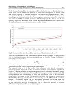
can be impacted again by land-use pattern changes. Figure 1 proposes a respective
conceptual framework for process-oriented land-use management.
A process-oriented land-use management must consider this network of processes and
interactions and is furthermore confronted with the challenge to bring together the three
pillars of sustainability (i) the ecological view emphasizing environmental and ecosystem
processes. On the other hand, also (ii) the economic view must be kept to optimize land-use
management planning and decision making. And (iii) the (regionally specific) societal
demands and frame conditions must be considered (Fürst et al., 2007a).
The DPSIR approach discussed e.g. by Mander et al. (2005) is a suitable and widely spread
methodological framework for dealing with environmental management processes in a
feedback loop, which controls the interactions within the cycle of Drivers–Pressures–State–
Impact–Responses. The DPSIR-approach, demands (i) for a set of suitable indicators and (b)
for process-models, which provide information on eco- and man-made system reactions
under changing (environmental) frame conditions. Climate change as an example is one of
the most important challenges for the future. Its complex impact on land-use management
and the potential of single land-use types to contribute in the future to socially requested

services and functions on landscape level are still under debate (Harrison et al., 2009; Prato,
2008, Metzger et al., 2006; Hitz & Smith, 2004). For supporting the integration of climate
change induced processes into sustainable land-use management decisions, both - indicators
and models - must be integrated into intelligent system solutions, which help to come to a
common understanding and acceptance of process-based management decisions.
2.1 Process-indicators
Suitable process indicators must be apt to describe course, direction and progress of
processes in single eco- or man-made systems. Furthermore, they should allow for an
upscaling of such processes on landscape level (Fürst et al., 2009; Zirlewagen, 2009;

Integration of Environmental Processes into Land-use Management Decisions

271
land-use
type 1
land-use
type 2
landscape
geology / soil types
topography
climate data
…
interactions
processes
land-user 1 land-user 2 land-user nland-user 1 land-user 2 land-user n
economy society
ecology
(natural and man made environment)
indicators
decision criteria

decisions

Fig. 1. Conceptual framework of process-oriented land-use management: land-use
management decisions consider the close connection of interactions and processes on
landscape level and are based on indicators, which reflect environmental processes and on
decision criteria resulting from the interacting land-users.
Zirlewagen & von Wilpert, 2009; Fürst et al., 2007b, Zirlewagen et al., 2007; Mander et al.,
2005). Finally, such indicators should also enable a comparative evaluation of processes in
different eco- or man-made systems to come to a holistic view on landscape level. (Wrbka et
al., 2004).
Herrick et al. (2006) highlightened the weakness of single indicators such as vegetation
composition to conclude on ongoing ecosystem processes and proposed to combine the
indicator vegetation composition with other process-indicators such as soil and site stability,
hydrologic function and biotic integrity. Fürst et al. (2007b) propose a framework of change-
ratio oriented indicators in forest ecosystems, which includes information on the natural
frame conditions, man-made changes and temporal development. Nigel et al. (2005)
analysed existing sets of criteria and indicators for biodiversity management impact in
forests and agricultural land-use and propose a landscape oriented approach how to
evaluate changes.
Concluding from research on appropriate process-indicators leads to the problem that process-
indicator-based management planning is not yet realizable in practice, because the necessary
holistic aggregation of single indicators or indicator sets from single ecosystems or land-use
types with focus on single landscape services is still in progress (Therond et al., 2008).
Process Management

272
2.2 Process-oriented management support tools and systems
To support the integration of environmental processes into management decisions, several
scientific and technological approaches are used. The challenge to integrate manifold
indicators and information as output of process-models into process-oriented decisions is

picked up by computer-based management and decision support systems (MSS, DSS). They
are drawing high attention as a means of improving the quality and transparency of
decision making in natural resource management (Rauscher, 1999). Beyond, an increasing
number of stakeholders, which are involved in natural resource management and the
resulting necessity to consider multiple interests and preferences in the decision-making
process led to the use of Multi-Criteria Decision Making (MCDM) techniques in DSS
development. Collaborative technologies such as Group Decision Support Systems (GDSS)
might help to avoid the consequences of knowledge fragmentation and will extend that
support to decision-making processes involving several individuals. Mendoza & Martins
(2006) remarked however that a paradigm shift is necessary in existing MCDM approaches
to come from methods for problem solving to methods for problem structuring to ensure
better support for the user.
Riolo et al. (2005) e.g. propose a combination of agent-based models and GIS to come to an
integration of spatio-temporal processes into management decisions. Castella & Verburg
(2007) tested a combination of process- and pattern-oriented models for decisions related to
land-use changes. Le et al. (2008) used a multi-agent based model for simulating spatio-
temporal processes in a coupled human–landscape system. From a review of existing multi-
agent models (MAS), Bousquet & Le Page (2004) came to the conclusion that these mostly
interdisciplinary approaches are helpful in complex decision situations.
However, Malczewski (2004) analysed appropriate systems for supporting the integration of
processes and process-knowledge into management decision and compared different tools
for GIS-based land-use suitability analysis. His analysis comprised methods such as GIS-
based modelling and overlay mapping, multicriteria decision making and artificial
intelligence methods (fuzzy logic, neural networks, cellular automatons, etc.). He
highlightened, that the major limitation of GIS-based modelling and overlapping is the lack
of well defined mechanisms for incorporating decision-makers preferences. Uran & Jansen
(2003) found additionally that the lack of user friendliness is the reason, why most of these
systems fail to be used in practice. According to Malczewski (2004), the main problem of
multicriteria decision making consists in the high variability of methods, which are applied
and the fact that the selection of different methods may produce different results.

Considering artificial intelligence methods, Malczewski (2004) criticised in general their
‘black box’ style, which makes it difficult for the user to understand how spatial problems
are analysed and how the results are produced.
Concluding from the research and comparison of existing tools and systems, (a)
transparency how environmental processes and interactions are handled in the approach
and how the results are produces, (b) user friendliness and (c) allowance for user dialog and
user interactions seem to be the most important features (see also Diez & McIntosh, 2009).
3. Pimp your landscape - a process-oriented management support tool
3.1 Idea and conception
“Pimp your landscape” (P.Y.L.) was designed to support the understanding of complex
interactions between various land-use types on landscape level and to provide a basis to
Integration of Environmental Processes into Land-use Management Decisions

273
evaluate the impact of user-made land-use pattern changes on most important land-use
services. Therefore, the continuous spatial problem “landscape” must have been divided
into spatially distinct units, which can interact and communicate with each other and to
which different attributes can be assigned.
The mathematical approach, which has been chosen to reflect complex spatial interactions,
was a cellular automaton with Moore-neighbourhood ship. Cellular automata were first
introduced by Ulam (1952) and their potential to support the understanding of the origin
and role of spatial complexity was highlightened by Tobler (1979). The approach was e.g.
used to model urban structures and land-use dynamics (Barredo et al., 2003; White et al.,
1996; White & Engelen, 1994, 1993), regional spatial dynamics (White & Engelen, 1997), or
the development of strategies for landscape ecology in metropolitan planning (Silva et al.,
2008). Nowadays, cellular automata are broadly used to simulate the impact of land-use
(pattern) changes and landscape dynamics (e.g. Moreno, et al., 2009; Wickramasuriya et al.,
2009; Yang et al., 2008; Holzkämper & Seppelt, 2007; Soares-Filho et al., 2002).
The starting point in P.Y.L. are land cover datasets, which are taken from Corine Landcover
(CLC) 2000 or national level (biotope type / land-use type maps). The smallest unit in the

P.Y.L. maps is the cell, which represents an area of 100x100 m² (CLC 2000) or 10x10 m² (only
special test sites based on land register maps). A cell can only be attributed with one land-
use type. Land-use types with a small share within a cell are assigned to the dominating
land-use type. Furthermore, multiple other attributes can be imported as geo-referenced
information layer (text or shape files) and can be assigned to the cells, such as geo-
pedological information, topographical parameters and climate characteristics. Also, linear
elements such as rivers, roads, railways or point-shaped elements of less than 100x100 m²
such as power plants can be assigned to a cell. Regarding point-shaped elements, the extent
of their spatial impact (e.g. deposition impact gradient) can be defined in the system.
Either it is possible to assign manually additional attributes to a cell, if digital information is
not available. In opposite direction, information from P.Y.L. can be exported as geo-
referenced text or shape file to a GIS.
The core of P.Y.L. is a hierarchical approach to evaluate the impact of land-use pattern
changes, which are induced by the user, on land-use services and functions (Fig. 2).
The evaluation starts by selecting the land-use types (biotope types / ecosystem types),
which are of regional relevance and by defining the land-use services and functions of
regional interest. The land-use classification standards of CLC 2000 and the land-use
services and functions (LUF) set described by Perez-Soba et al. (2008) are available as initial
settings. The user can modify these initial settings or adopt completely different settings
according to the regional application targets.
In a next step, indicator sets are identified, which provide information on the impact of the
land-use types on land-use services and functions. This step requires several feed-back loops
with regional experts: a major problem in the holistic evaluation on landscape level consists
(a) in the different scales and dimensions of indicator sets at the different land-use types
(Fürst et al., 2009) and (b) in the regional availability of respective knowledge sources.
Therefore, a meaningful selection and weighting of the indicators is requested, which
respects also regional expert knowledge and experiences to compensate existing knowledge
gaps.
Based on the indicator sets, the impact of each land-use type on each land-use service or
function is evaluated on a relative scale from 0 (worst case) to 100 (best case). The

introduction of this relative scale enables (a) to compare the impact of different land-use

Process Management

274
evaluation result
at different time slots
evaluation of
land-use pattern changes at tn
regionalized evaluation
cell specific adjustment
neighborhood relationships environmental conditions
initial (regional) value table
user
expert
landscape structure (indices)
planning regulations & restrictions
land-use type 1 land-use type 2 land-use type 3 land-use type n
indicator l1.1
indicator l1.2
indicator l1.n
indicator l2.1
indicator l2.n
indicator l3.1
indicator l3.n
indicator l4.1
indicator l4.2
indicator l4.3
indicator l4.4
tn - m

tn - o tn - p
expert knowledge
experiences

Fig. 2. Hierarchical evaluation of the impact of land-use pattern changes.
types on an individual land-use service or function. (b) The setting of a relative scale as
reference supports also a multifunctional evaluation, which faces the challenge to make
comparable reactions of different land-use services and functions on land-use pattern
changes.
The resulting (regional) value table represents initial impact values of the land-use types on
the services and functions. These must be regionalized to consider (a) the cell specific
environmental frame conditions (e.g. height above sea level, mean annual precipitation and
temperature, soil type and exposition) and (b) the neighbourhood of different land-use
types. This step is supported by rule-sets, which offer the user the possibility to specify a
possible increase or decrease of the initial value in dependence from neighbourhood type
(homogeneous land-use types Ù different land-use types, edge to edge Ù corner to corner)
and in dependence from the (available) environmental attributes.
Building upon the regionalized evaluation basis, landscape structure indices (landscape
metrics) are introduced to adopt the evaluation of “soft” land-use services and functions
Integration of Environmental Processes into Land-use Management Decisions

275
referring to biodiversity or services related to the aesthetical value of a landscape. The
indices help to integrate the heterogeneity of the land- use pattern, the size and connectivity
of patches and the form of patches from the holistic landscape view (e.g Uuemaa et al.,
2009).
In addition, the user is offered various options to insert regional planning rules and
restrictions. These limit the degree of freedom to which the land-use pattern can be
modified.
The user can specify (a) rules in dependence from the land-use pattern, such as if a land-use

type can be converted into another, if a land-use type restricts the conversion of a
neighbouring land-use type or if a linear element (street, water body) restricts the
conversion of the land-use type at the cell to which this element is assigned.
Also rules for the spatial development of a land-use type can be defined, such as minimum
or maximum thresholds and growth trends, i.e. if the share of a land-use type can increase,
decrease or should remain equal.
(b) Rules depending from environmental frame conditions can be specified, such as if a
land-use type is allowed to be converted into another in dependence from pedo-geological,
topographical or climatic attributes. Here, the user can choose between the definition of
value ranges of the attributes and the definition of upper or lower thresholds.
(c) Thresholds for the selected land-use services and functions can be defined. According to
the evaluation logic, these must adopt a value between 0 and 100.
Taking the rules into account, the user can start the simulation and can start to modify the
land-use pattern. He receives a feed-back on the impact of his changes on the land-use
services and functions in real time: the system sums up the value of each cell for each land-
use type and divides these sums by the total number of cells, which are displayed in the
simulation. A mean value is calculated for each land-use service and the evaluation result is
displayed as star diagram.
The evaluation result is based on the assumption that each land-use type as soon as it is
established has its full impact on the land-use services and functions (time point tn). To
come to a more realistic evaluation, the possibility to switch between the evaluation results
at different time slots of 10, 30, 50 and 100 years is actually integrated into the system (time
points tn-m, … tn-p).
3.2 Application areas and examples
P.Y.L. allows the user to test the complex and various effects of land-use pattern changes
and the establishment of linear and point-shaped infrastructural elements on land-use
services and functions by simple mouse click (Fig. 3).
The user can conduct local changes (cell by cell, freehand shape, establishment of a point-
shaped element) or regional changes (changing all cells of a land-use type / changing all
cells of a land-use type, which are spatially connected, establishment of linear elements).

In the philosophy of the system, natural transition processes between land-use types or
ecosystems are not considered: the vision of the system is to teach the user the
understanding of the effects of his actions on landscape level without additional impact
factors, which he cannot influence.
In land-use management planning, P.Y.L. is adapted and tested for different application
areas:
Process Management

276

simulation | definition | create maps | import maps | upload maps | define planning restrictions | define environmental restrictions | support and FAQ´s
map: env. restriction: evaluation | thresholds land-use services & functions
state | changes
save
5 min
display original map


Fig. 3. Graphical user interface of P.Y.L. with variable options to modify the land-use pattern
and to introduce linear / point-shaped elements (icons).
a. testing the effects of a regional application of rules and restrictions derived from EU
regulations, such as EU Water Framework Directive (2000/60/EC) and Natura 2000
(79/409/EEC and 92/43/EEC) on regionally important land-use services and functions
b. testing different planning alternatives for the spatial development of urban areas and
the establishment of infrastructural facilities, such as highways, railways and roads and
deriving the extent of possible compensation measures to keep a politically / socially
requested level of land-use services and functions such as live quality, biodiversity, etc.
c. testing the effects of flooding in the frame of open cast mining area restoration and of
participatory elements in landscape planning (recreation areas and areas reserved for
natural succession vs. establishment of touristic infrastructure)

d. testing the effects of climate change on regional risks and potentials and on possible
mitigation strategies through changes in the land-use.
In case (a) - (c), additional effects of changing climatic frame conditions are considered,
while responses to climate change are the focal point in case (d).
Considering (d), the impact of different climate change scenarios is currently tested at the
model region “Dresden” (Saxony /Germany) in the project REGKLAM (Development and
Testing of an Integrated Regional Climate Change Adaptation Programme for the Model
Region of Dresden, www.regklam.de). Regionalized climate change scenarios are combined
with soil and topographical data to derive scenario specific risk maps for erosion and
drought. These are used as layers in P.Y.L. instead of primary climate, geological and
Integration of Environmental Processes into Land-use Management Decisions

277
topographical parameters. In a first step and based on a region specific evaluation, it is
tested, how the actual land-use pattern increases or decreases the drought and erosion risk.
In a next step, planning scenarios for urban growth, spatial development of forestry and
agriculture are combined with the risk maps to get (a) information on possible range of
responses to regional climate change impact by land-use pattern changes and (b) on areas,
where additionally land-use type specific changes in management are demanded.
Figs. 4a - 4b show a typical run at the model region Leipzig (Saxony / Germany), where the
effects of building a highway are evaluated on regional level (4a) and with local focus (4b)
and where a compensation measure (increase of regional forests from 12 to 30 %, 4c) and
finally the possible impact of the construction of a lignite power plant with well described
gradient (4d) are tested. The star diagram displays the effects of the planning measures for
five regionally selected landscape services, the drinking water quality, the aesthetical value
of the landscape, climate change sensitivity (based upon regionalized climate change
scenarios), regional economy and human health.
The example reveals also a still existent problem in the evaluation: the impact of linear
elements on a region (based on the model of a cellular automaton) is hardly appraisable.
Here, the switch between two evaluation perspectives, the regional one (Fig. 4a) and the

local one (Fig. 4b) helps to approximate to the impact of this planning measure. On the other
hand, the increase of the forest area seems to overcompensate the highway construction and
also the power plant construction. Here, the adjustment of the evaluation result by
landscape metrics is still outstanding.

drinking water quality
aesthetical
value
dlimate change adaptivityregional economy
human
health


Fig. 4a. Test of the impact of a highway construction on regional level.
Process Management

278
Area Focus
regional economy dlimate change adaptivity
drinking water quality
aesthetical
value
human
health

Fig. 4b. Switch to the local impact of the highway with focus on a planned motorway
junction.
drinking water quality
aesthetical
value

dlimate change adaptivityregional economy
human
health

Fig. 4c. Test of a large scale compensation measure by increasing the share of forest land
from 12 to ca. 30 %.
Integration of Environmental Processes into Land-use Management Decisions

279
drinking water quality
aesthetic
a
value
dlimate change adaptivityregional economy
human
health

Fig. 4d. Testing of the sensitivity of the compensation measure “afforestation” against the
additional establishment of a power plant with western deposition gradient.
4. Discussion and conclusions
“Pimp your landscape (P.Y.L.)” was developed since 2007 to support process-knowledge
integration into land-use management planning decisions on landscape level (Fürst et al.,
2008). The integration of process-knowledge is realized by several characteristics of the system:
a. the mathematical approach of a cellular automaton enables to simulate by a set of rules
dynamic interactions between land-use types and to consider the spatial complexity at
landscape level (White et al., 1997).
b. GIS features of P.Y.L. enable to overlay various land-use pattern scenarios with various
environmental parameters, which can also be scenario-driven, such as e.g. climate data
(as primary data set) or risk maps (as secondary data set) etc.
c. The evaluation approach comprises a complex bundling process of indicators and

expert knowledge, which is highly sensible for specific regional demands, changing
evaluation targets and variable societal demands.
d. The process of changing the land-use pattern and adding linear of point-shaped
elements with their resulting impact on land-use services and functions is strictly
driven and defined by the user on the basis of his planning questions and the planning
alternatives, he wants to test. Therefore, the criterion transparency is given and as
requested by Mendoza & Martins (2006), “decision making” is replaced by support in
“problem structuring and testing”.
Compared to complex spatial decision or management support approaches, P.Y.L. is based
on knowledge, which might be derived from modelling, but takes its results not by coupling
Process Management

280
of models as e.g. done by Le et al. (2008) or Castella et al. (2007). Therefore, also no transition
probabilities between different land-use types and historical land-use development can be
simulated. This shortcoming in applicability to real world was tolerated with regard to the
intention to make better understandable the effects of user-driven land-use pattern changes.
The requested complex process of knowledge bundling and the identification and selection
of indicators and their combination with expert knowledge and experiences must be
moderated by science individually for each region and can only build upon results from
comparable regions. Furthermore, the use of a relative scale from 0 to 100 to evaluate the
impact of land-use changes on land-use services and functions gives no quantitative, but
only qualitative information. A resulting risk, which is not specific for P.Y.L. but applies for
all knowledge management and decision support systems, is the improper parameterization
and use and hereby derived inaccurate decisions (Richardson et al., 2006). However, if the
evaluation process is managed well under close participation of regional experts and with
detailed documentation of the knowledge sources, the evaluation results in P.Y.L. can
experience a high regional acceptance. The easy adaptation of the evaluation base and the
rule systems supports also testing how the “system landscape” reacts under variable
assumptions on the future value of land-use types for land-use services and functions.

Finally, a possible problem can occur in the case that P.Y.L. is used at different scale levels in
a region, as actually tested in the frame of the REGKLAM project. Moreno et al. (2009) e.g.,
highlighten the sensitivity of cellular automata to cell size and neighbourhood
configuration. Furthermore, problems in the classification logic can appear, when assigning
land-use types over different scale levels to the dominating land-use type in a cell. Last but
not least, also landscape metrics react sensible on scale level changes (Pascual-Hortal &
Saura, 2007; Uuema et al., 2005). Here, approaches how to bridge scale level problems and
recommendations for the proper use of the system are actually under development.
5. References
Barredo, J.I.; Kasanko, M.; McCormick, N.; Lavalle, C. (2003). Modelling dynamic spatial
processes: simulation of urban future scenarios through cellular automata.
Landscape and Urban Planning, 64(3), pp.145-160
Bengtsson, J.; Nilsson, S.G.; Franc, A.; Menozzi. P. (2000). Biodiversity, disturbances,
ecosystem function and management of European forests. Forest Ecology and
Management, 132(1), pp. 39-50.
Bonsall, C.; Macklin, M. G.; Anderson, D. E.; Payton, R. W. (2002). Climate Change and the
Adoption of Agriculture in North-West Europe. European Journal of Archaeology,
5(1), pp.9-23
Botequilha Leitao, A. & Ahern, J. (2002). Applying landscape ecological concepts and
metrics in sustainable landscape planning. Landscape and Urban Planning, 59(2),
pp.65-93
Bousquet, F. & Le Page, C. (2004). Multi-agent simulations and ecosystem management: a
review. Ecological Modelling, 176(3), pp.313-332
Bytnerowicz, A.; Omasa, K.; Paoletti, E. (2007). Integrated effects of air pollution and climate
change on forests: A northern hemisphere perspective. Environmental Pollution,
147(3), pp.438-445
Integration of Environmental Processes into Land-use Management Decisions

281
Callaghan, T.V.; Björn,L.O.; Chernov, Y.; Chapin, T.; Christensen, T.R. ; Huntley, B.; Ims, R.

A.; Sitch, S. (2004). Effects of changes in climate on landscape and regional
processes, and feedbacks to the climate system. Ambio, 33(7), pp.459-468
Castella, J.C. & Verburg, P.H. (2007). Combination of process-oriented and pattern-oriented
models of land-use change in a mountain area of Vietnam. Ecological Modelling,
202(3), pp.410-420
Castella, J C.; Pheng Kam, S.; Dinh Quang, D.; Verburg, P.H.; Thai Hoanh, C. (2007).
Combining top-down and bottom-up modelling approaches of land use/cover
change to support public policies: Application to sustainable management of
natural resources in northern Vietnam. Land Use Policy, 24(3), pp.531-545
Demirbas, A. (2009). Political, economic and environmental impacts of biofuels: A review.
Applied Energy, 86, pp.S108-S117
Diez, E. & McIntosh, B.S. (2009). A review of the factors which influence the use and
usefulness of information systems. Environmental Modelling and Software, 24(5),
pp.588-602
Dragosits, U.; Theobald, M.R.; Place, C.J.; ApSimon, H.M.; Sutton, M.A. (2006). The potential
for spatial planning at the landscape level to mitigate the effects of atmospheric
ammonia deposition. Environmental Science and Policy, 9(7-8), pp. 626-638
Garcia-Gonzalo, J.; Peltola, H.; Briceno-Elizondo, E.; Kellomaki, S. (2007). Effects of climate
change and management on timber yield in boreal forests, with economic
implications: A case study. Ecological Modelling, 209(2), pp.220-234
Fürst, C.; Zirlewagen, D.; Lorz, C. (2009). Regionalization of magnetic susceptibility
measurements based on a multiple regression approach. Water, Air, and Soil
Pollution, doi: 10.1007/s11270-009-0154-1
Fürst, C.; Davidsson, C.; Pietzsch, K.; Abiy, M.; Makeschin, M.; Lorz, C.; Volk, M. (2008).
“Pimp your landscape” – interactive land-use planning support tool. Transactions
on the Built Environment (ISSN 1743-3509). Geoenvironment and Landscape Evolution,
III, pp. 219-232.
Fürst, C.; Vacik, H.; Lorz, C.; Makeschin, F.; Podraszky, V.; Janecek, V. (2007a): Meeting the
challenges of process-oriented forest management. Forest Ecology and Management,
248(1-2), pp. 1-5

Fürst, C.; Lorz, C.; Makeschin, F. (2007b): Development of forest ecosystems after heavy
deposition loads considering Dübener Heide as example - challenges for a process-
oriented forest management planning. Forest Ecology and Management, 248(1-2), pp.
6-16
Goetz, S.J.; Mack, M.C.; Gurney, K.R.; Randerson, J.R.; Houghton, R.A. (2007). Ecosystem
responses to recent climate change and fire disturbance at northern high latitudes:
observations and model results contrasting northern Eurasia and North America.
Environmental Research Letters, 2(4), p.045031
Harrison, P.; Rounsevell, M., Luck, G.; Harrington, R.; Sykes, M.; Vandewalle, M. (2009). A
conceptual framework to analyse the effects of environmental change on ecosystem
services. IOP Conference Series: Earth and Environmental Science, 6(30), p.302017,
doi:10.1088/1755-1307/6/30/302017
Herrick, J.E.; Schuman, G.E.; Rango, A. (2006). Monitoring ecological processes for
restoration projects. Journal for Nature Conservation, 14(3), pp.161-171
Hitz, S. & Smith, J. (2004). Estimating global impacts from climate change. Global
Environmental Change, 14(3), pp.201-218
Process Management

282
Holzkämper, A.; Seppelt, R. (2007). A generic tool for optimizing land-use patterns and
landscape structures. Environmental Modelling & Software, 22, pp.1801-1804
Jessel, B. & Jacobs, J. (2005). Land use scenario development and stakeholder involvement as
tools for watershed management within the Havel River Basin. Limnologica -
Ecology and Management of Inland Waters, 35(3), pp. 220-233.
Kallioras, A.; Pliakas, F.; Diamantis, I. (2006.) The legislative framework and policy for the
water resources management of trans-boundary rivers in Europe: the case of
Nestos/Mesta River, between Greece and Bulgaria. Environmental Science and Policy,
9(3), pp. 291-301
Kellomäki, S.; Peltola, H.; Nuutinen, T.; Korhonen, K.T.; Strandman, H. (2008). Sensitivity of
managed boreal forests in Finland to climate change, with implications for adaptive

management. Philosophical Transactions of the Royal Society B: Biological Sciences,
363(1501), pp. 2341-2351
Le, Q.B.; Park, S.J.; Vlek, P.L.G.; Cremers, A.B. (2008). Land-Use Dynamic Simulator
(LUDAS): A multi-agent system model for simulating spatio-temporal dynamics of
coupled human–landscape system. I. Structure and theoretical specification.
Ecological Informatics, 3(2), pp.135-153
Letcher, R.A. & Giupponi, C. (2005). Policies and tools for sustainable water management in
the European Union. Environmental Modeling and Software, 20(2), pp. 93-98
Lindner, M. & Kolström M. (2009). A review of measures to adapt to climate change in
forests of EU countries, IOP Conference Series: Earth and Environmental Science, 6 (38),
p.382007, doi:10.1088/1755-1307/6/38/382007
Malczewski, J. (2004). GIS-based land-use suitability analysis: a critical overview. Progress in
Planning, 62(1), pp.3-65
Mander, Ü.; Wiggering, H.; Helming, K. (2007). Multifunctional land use - meeting future
demands for landscape goods and services. pp. 1-14. Springer. Berlin.
Mander, Ü.; Müller, F.; Wrbka, T. (2005). Functional and structural landscape indicators:
upscaling and downscaling problems. Ecological Indicators, 5 (2005), pp. 267–272
Mendoza, G.A. & Martins, H. (2006). Multi-criteria decision analysis in natural resource
management: A critical review of methods and new modelling paradigms. Forest
Ecology and Management, 230(1), pp.1-22
Metzger, M.J.; Rounsevell, M.D.A.; Acosta-Michlik, L.; Leemans, R.; Schroter, D. (2006). The
vulnerability of ecosystem services to land use change. Agriculture, Ecosystems and
Environment, 114(1), pp.69-85
Miraglia, M.; Marvin, H.J.P.; Kleter, G.A.; Battilani, P.; Brera, C.; Coni, E.; Cubadda, F.;
Dekkers, S. (2009). Climate change and food safety: An emerging issue with special
focus on Europe , Food and Chemical Toxicology, 47(5), pp.1009-1021
Moreno, N.; Wang, F.; Marceau, D.J. (2009). Implementation of a dynamic neighborhood in a
land-use vector-based cellular automata model. Computers, Environment and Urban
Systems, 33(1), pp.44-54
Niemelä, J.; Young, J.; Alard, A.; Askasibar, M.; Henle, K.; Johnson, R.; Kurttila, M.; Larsson,

T.B.; Matouchi, S.; Nowicki, P.; Paiva, R.; Portoghesil, L.; Smulders, R.; Stevenson,
A.; Tartes, U.; Watt., Q. (2005). Identifying managing and monitoring conflicts
between forest biodiversity conservation and other human interests in Europe.
Forest Policy and Economics, 7(6), pp. 877-890.
Integration of Environmental Processes into Land-use Management Decisions

283
Nigel, D.; Baldock, D.; Nasi, R.; Stolton, S. (2005). Measuring biodiversity and sustainable
management in forests and agricultural landscapes. Philosophical Transactions of the
Royal Society B: Biological Sciences, 360 (1454), pp.457-470
Olesen, J.E. & Bindi, M. (2002). Consequences of climate change for European agricultural
productivity, land-use and policy European. Journal of Agronomy, 16(4), pp.239-262
Pascual-Hortal, L. & Saura, S. (2007). Impact of spatial scale on the identification of critical
habitat patches for the maintenance of landscape connectivity. Landscape and Urban
Planning, 83(2), pp.176-186
Perez-Soba, M.; Petit, S.; Jones, L.; Bertrand, N.; Briquel, V.; Omodei-Zorini, L.; Contini, C.;
Helming, K.; Farrington, J.; Tinacci-Mossello, M.; Wascher, D.; Kienast, F.; de
Groot., R. (2008). Land use functions – a multifunctionality approach to assess the
impacts of land use change on land use sustainability. In Helming, K.; Tabbush, P.;
Perez-Soba, M. (Ed.) Sustainability impact assessment of land use changes. pp.375-404,
Springer Berlin-Heidelberg
Prato, T. (2008). Conceptual framework for assessment and management of ecosystem
impacts of climate change. Ecological Complexity, 5(4), p.329-338
Rauscher, H.M. (1999). Ecosystem management decision support for federal forests in the
United States: A review. Forest Ecology and Management, 114(2), pp. 173-197
Richardson, S.M.;/ Courtney, J.F.; Haynes, J.D. (2006). Theoretical principles for knowledge
management system design: Application to pediatric bipolar disorder. Decision
Support Systems, 42 (3), pp.1321-1337
Riolo, R.; Brown, D,G.; Robinson, D.T.; North, M.; Rand, W. (2005). Spatial process and data
models: Toward integration of agent-based models and GIS. Journal of Geographical

Systems, 7(1), pp. 25-47
Schulp, C.J.E.; Nabuurs, G.J.; Verburg, P.H. (2008). Future carbon sequestration in Europe-
Effects of land-use change. Agriculture, Ecosystems and Environment, 127(3), pp.251-264
Silva, E.A.; Ahern, J.; Wileden, J. (2008). Strategies for landscape ecology: An application
using cellular automata models. Progress in Planning, 70(4), pp.133-177
Soares-Filho, B.S.; Coutinho Cerqueira, G.; Lopes Pennachin, C. (2002). dynamica—a
stochastic cellular automata model designed to simulate the landscape dynamics in
an Amazonian colonization frontier. Ecological Modelling, 154(3), pp.217-235
Stoeglehner, G. & Narodoslawsky, M. (2009). How sustainable are biofuels? Answers and
further questions arising from an ecological footprint perspective. Bioresource
Technology, 100(16), pp.3825-3830
Tenhunen, J.; Geyer, R.; Adiku, S.; Reichstein, M.; Tappeiner, U.; Bahn, M.; Cernusca, A.;
Dinh, N.Q.; Kolcun, O.; Lohila, A.; Otieno, D.; Schmidt, M.; Schmitt, M.; Wang, Q.;
Wartinger, M.; Wohlfahrt, G. (2009). Influences of changing land-use and CO2
concentration on ecosystem and landscape level carbon and water balances in
mountainous terrain of the Stubai Valley, Austria. Global and Planetary Change,
67(1), pp.29-43
Therond, O.; Turpin, N.; Belhouchette, H.; Bezlepkina, I.; Bockstaller, C.; Janssen, S.J.C.;
Alkan-Olsson, J.; Bergez, J-E.; Wery, J.; Ewert, F. (2008). How to manage models
outputs aggregation for indicator quantification within SEAMLESS integrated
framework, In: Proceedings of Impact Assessment of Land Use Changes. April 6-9, 2008,
Berlin, Germany. - Berlin : Humboldt University
Tobler, W. (1979). Cellular geography. In: Gale, S.; Olsson, G.: Pilosophy in Geography, pp.
379-386, Reidel Publisher, Dordrecht
Process Management

284
Ulam, S. (1952). Random processes and transformations. Proceedings of the International
Congress on Mathematics (2), pp. 264-275, American Mathematical Society,
Providence RI

Uran, O. & Janssen, R. (2003). Why are spatial decision support systems not used? Some
experiences from the Netherlands. Computers, Environment and Urban Systems, 27,
pp. 511–526
Uuemaa M. A.; Roosaare J.; Marja R.; Mander U. (2009). Landscape Metrics and Indices: An
Overview of Their Use in Landscape Research. Living Reviews of Landscape Research,
3(1). [Online Article]: cited 28.10.2009,
Uuemaa, E.; Roosaare, J.; Mander, U. (2005). Scale dependence of landscape metrics and
their indicatory value for nutrient and organic matter losses from catchments.
Ecological Indicators, 5(4), pp.350-369
Van Delden, H.; Luja, P.; Engelen, G. (2007). Integration of multi-scale dynamic spatial
models of socio-economic and physical processes for river basin management.
Environmental Modeling and Software, 22(2), pp. 223-238
White, R. & Engelen, G. (1997). Cellular automata as the basis of integrated dynamic
regional modelling. Environment and Planning B: Planning and Design, 24, pp. 235-
246
White, R. & Engelen, G. (1994). Urban systems dynamics and cellular automata: Fractal
structures between order and chaos. Chaos, Solitons and Fractals, 4 (4), pp.563-583
White, R. & Engelen, G. (1993). Cellular automata and fractal urban form: a cellular
modelling approach to the evolution of urban land-use patterns. Environment and
Planning A, 25, pp. 1175-1199
White, R.; Engelen, G.; Uljee, I. (1997): The use of constrained celluar automata for high-
resolution modelling of urban land-use dynamics, Environment and Planning B:
Planning and Design 24, pp 323-343
Wickramasuriya, R.C.; Bregt, A.K. van Delden, H.; Hagen-Zanker, A. (2009). The dynamics
of shifting cultivation captured in an extended Constrained Cellular Automata land
use model. Ecological Modelling, 220(18), p.2302-2309
Wiggering, H.; Dalchow, C.; Glemnitz, M.; Helming, K.; Müller, K.; Schulz, A.; Stachow, U.;
Zander, P. (2006). Indicators for multifunctional land use - Linking socio-economic
requirements with landscape potentials. Ecological Indicators, 6, pp. 238-249
Wrbka, T.; Erb, K H.;/ Schulz, N.B.; Peterseil, J.; Hahn, C.; Haberl, H. (2004). Linking

pattern and process in cultural landscapes. An empirical study based on spatially
explicit indicators. Land Use Policy, 21(3), pp.289-306
Yang, Q. & Li, X. / Shi, X. (2008). Cellular automata for simulating land use changes based
on support vector machines. Computers and Geosciences, 34(6), pp.592-602
Zirlewagen, D. (2009). Regionalisierung der bodenchemischen Drift in der Dübener Heide
im Zeitraum 1995–2006. Waldökologie, Landschaftsforschung und Naturschutz, 8, pp.
21-30
Zirlewagen, D. & Wilpert, K. von (2009). Raum-Zeitmuster von Stoffflüssen im Boden:
Verbindung von Sickerwasserchemie und Bodenfestphase, Waldökologie,
Landschaftsforschung und Naturschutz, 8, pp. 31-40.
Zirlewagen, D.; Raben, G.; Weise, M. (2007). Zoning of forest health conditions based on a
set of soil, topographic and vegetation parameters. Forest Ecology & Management,
248(1–2), pp. 43-55.
16
Guidelines to Improve Construction and
Demolition Waste Management in Portugal
Armanda Couto and João Pedro Couto
University of Minho
Portugal
1. Introduction
The construction industry is a major contributor to excessive natural resource consumption,
depletion and degradation; waste generation and accumulation; and environmental impact
and degradation. The amount of waste generated by the construction and demolition
activity is substantial. Surveys conducted in several countries found that it is as high as 20%
to 30% of the total waste entering landfills throughout the world (Bossink & Brouwers,
1996). Moreover, the weight of the generated demolition waste is more than twice the
weight of the generated construction waste. Other studies compared new construction to
refurbishment, and concluded that the latter accounts with more than 80% of the total
amount of waste produced by the construction activity as a whole. The building activity at
historical city centres tends to be an important waste generator because both refurbishment

projects and new projects often include demolition (Teixeira & Couto, 2000). Construction
site activities in urban areas may cause damage to the environment, interfering with the
daily life of local residents, who frequently complain about dust, mud, noise, traffic delay,
space reduction, materials or waste deposition in the public space, etc. Regarding this
theme, an attempt was made to order each impact by the importance given to each one in
scientific publications, being the following the most frequently mentioned (Couto, 2002;
Couto & Couto, 2006):
• Production of waste;
• Mud on streets;
• Production of dust;
• Soil and water contamination and damaging of the public drainage system;
• Damaging of trees;
• Visual impact;
• Noise;
• Increase in traffic volume and occupation of public roads; and
• Damaging of the public space.
A recent research study carried out by the Instituto Superior Técnico da Universidade
Técnica de Lisboa (Technical University of Lisbon) reveals that most of the construction and
demolition (C&D) waste is not recycled in Portugal in opposition to what is happening in
most European Countries. This study advances that Portugal generates around 4.4 million
tones (Mt) per year of core C&D. However, in most construction sites the waste is selected
Process Management

286
but its destination is not controlled. Only a few local authorities require the promoters to
make a plan for C&D waste (Couto & Couto, 2009).
This inappropriate management for long time has lead to the appearing of many disposals
in green areas, adjoining roads and other sensible places.
On the other hand, there is not yet a market for recyclable materials. Most practitioners have
been manifesting distrust and lack of information about this issue.

In the Historical City Centres (HCC) the negative effects of the construction projects have
even a greater relevance, since they are urban areas with very particular characteristics. As
they are touristic locations, it is necessary to maintain them as much as possible as pleasant
places to live, work and enjoy. Furthermore, these areas frequently have significant
restrictions regarding the available space, which brings about more difficulties for the
construction projects. Therefore, the HCC, in view of their specificities, require a special
attention from the intervenients of the construction sector in order to minimize the impacts
of the construction projects.
The national inquiry carried out with the Portuguese Association of Cities with Historical
Centers (Couto, 2002; Teixeira & Couto, 2002), of which 50% of members (56) answered, had
the results showed in table 1 regarding the most common prevention attitudes towards the
waste impact.


Common prevention attitude - waste

Answers (%)
Generally Compulsive Prevention –
in the licensing of the construction project
according to municipal norms/regulations
54
Sporadically Require Prevention –
in the licensing of the construction project, in
some circumstances
29
Eventually Require Prevention –
during the work execution due to complaints
from affected citizens
14
Without Prevention –

considering the inconveniences caused by the
normal execution of the construction project
3
Table 1. Common prevention attitudes towards waste production impact
The result shows that only about half of the respondents have expressed that preventive
measures are generally required in the licensing stage, which is quite worrying due to the
importance and sensibility of those places. The lack of a preventive attitude from both the
authorities and the contractors, followed by an inefficient inspection and control by the
authorities are the main causes for the majority of complains from neighbors and transients.
This work presents a strategic actions set necessary to improve and promote the waste
construction management in Portugal. An effort should be made in order to reduce waste
production on site and to increase its recycling value. The reuse, based on deconstruction
process, should be considered a good solution and an opportunity market.