Heat Conduction Basic Research Part 12 pptx

Heat Conduction – Basic Research

264

0
()
||
() ()exp(||| |) exp(||( ))d ,
*( ) 4 ( )
A
uA
fy
is
fy f s y sy
sEy Gy




      




0
*( )
1exp(||)
() (s
g
n( ) 1) ( )

22()*()
v
s
yy
GE








   





0
||
()exp(||| |) exp(||( ))d d,
4()
s
ss
Gy

   








0
*( )
1
() (s
g
n( ) 1) *()() ()
2*()
v
yy T
E


  



   





0
||
()exp(||| |) exp(||( ))d d,

4()
s
ss
Gy

   







0
*( )
1
() (s
g
n( ) 1) ( )
2*()
vA
fy y f
E






  






0
||
()exp(||| |) exp(||( ))d d.
4()
A
s
fs s
Gy

   







Formulae (47) present the expression for determination of the displacement-vector
components in the inhomogeneous semi-plane due to given external tractions
p
and q ,
and the temperature field
()Ty .
3.2.3 One-to-one relations between the tractions and displacements on the boundary
Putting 0y  into (45) and (46), we obtain the relations

0
0
(0),
d(0)
(0) .
d
x
x
xy
i
u
s
i
isv
sy






Having substituted the corresponding physical relations (33) into the latter relations, we
arrive at the following one-to-one relations

011 12 1
021222
,uapaqb
vapaqb




(48)
between the tractions and displacements on the boundary of semi-plane D. Here
11 12 1
2
11 1
,,*(0)(0),
|| *(0) 2 (0)
*(0 )
ii
aabT
ssE G s
sE


   




Steady-State Heat Transfer and Thermo-Elastic Analysis of Inhomogeneous Semi-Infinite Solids

265
21
2
() () exp(||)
1d 1
(0)
d *() || (0)*() 2()
A

A
y
fy sy
a
yEy s f Ey Gy
s



 






0
0
()
|| 1
() (0) exp(||| |) exp(||( ))d ,
4() || (0)
A
A
y
f
s
sy sy
Gy s f








 











21
2
0
0
()
d1
(0) d *( )
(0)
||
()exp(||| |) exp(||( ))d ,
4()
A

A
A
y
fy
ii
a
sG y s E y
sf
s
fsy sy
sG y
 












2
2
() ()
1d (0)
*( ) ( )
d*()(0)*()

A
A
fy y
byTy
yEyf Ey
s









0
0
|| (0)
() () exp(||| |) exp(||( ))d .
4() (0)
A
A
y
s
fsy sy
Gy f
  






 







The obtained expressions of (48) allow us to determine the displacements on the boundary
through the given tractions, and vice-versa.
3.2.4 Case B: Boundary condition in terms of displacement
Consider the problem of thermoelasticity (31) – (34), (36), where the boundary
displacements
0
()ux and
0
()vx are given, meanwhile, the corresponding boundary
tractions
()
p
x and ()qx are to be determined. By solving (48) with respect to
p
and q , we
find the transforms of tractions on the boundary through the displacements as

22 12 12 2 22 1
00
21 11 21 1 11 2

00
,
,
aaabab
puv
aaabab
quv
 
 



  
(49)
where
11 22 12 21
.aa aa

 Having determined the boundary tractions (49), we can find the
stress-tensor components by formulae (38), (40), and the displacement-vector components
by formulae (47).
3.2.5 Case C: Solution of the problem with mixed boundary conditions
Finally, we consider the thermoelasticity problem (31) – (34) in the semi-plane D, when
mixed boundary conditions of either the type (37) are imposed on the boundary. For four
versions of the mixed boundary conditions (37), by making use of one of the relations (48),
we express the Fourier transform of the unknown traction in terms of the given functions on
the boundary and the temperature; inserting the expression into (38) and (40), we calculate
the stresses and eventually the displacements by formula (47).

Heat Conduction – Basic Research

266
4. Conclusions
Using the method of direct integration, the explicit-form analytical solutions have been
found for the equations of in-plane heat conduction and plane thermoelasticity problems in
an inhomogeneous semi-plane provided the tractions, displacement, and mixed conditions
are prescribed on the boundary. Due to the fact that the application of technique for
reducing the aforementioned equations to the governing Volterra-type integral equations
with further employment of the resolvent-kernel solution algorithm provides us with the
explicit-form solutions of the thermoelasticity problems, the one-to-one relations between
the tractions and the displacements on the boundary of the semi-plane are derived. Making
use of these relations, we have reduced quasi-static boundary value problems of the plane
theory of thermoelasticity with displacement or mixed boundary conditions to the solution
of the problem when the tractions are prescribed on the boundary. Application of this
technique does not impose any restrictions for the functions prescribing the material
properties (besides existence of corresponding derivatives, at least, in generalized sense).
But from mechanical point of view, it can be concluded, that the material properties should
be in agreement with the model of continua mechanics assuring strain-energy within the
necessary restrictions.
5. Acknowledgment
The authors gratefully acknowledge the financial support of this research by the National
Science Council (Republic of China) under Grant NSC 99-2221-E002-036-MY3.
6. References
Bartoshevich, M.A. (1975). A Heat-Conduction Problem. Journal of Engineering Physics and
Thermophysics, Vol.28, No.2, (February 1975), pp. 240-244, ISSN 1062-0125
Belik, V.D., Uryukov, B.A., Frolov, G.A., & Tkachenko, G.V. (2008). Numerical-Analytical
Method of Solution of a Nonlinear Unsteady Heat-Conduction Equation. Journal of
Engineering Physics and Thermophysics, Vol.81, No.6, (November 2008), pp. 1099-
1103, ISSN 1062-0125
Brychkov, Yu.A. & Prudnikov, A.P. (1989). Integral Transforms of Generalized Functions,

Gordon & Breach, ISBN: 2881247059, New York, USA
Carslaw, H.S. & Jaeger, J.C. (1959). Conduction of Heat in Solids, Oxford University Press,
ISBN: 978-0-19-853368-9, London, England
Domke, K. & Hącia, L. (2007). Integral Equations in Some Thermal Problems, International
Journal of Mathematics and Computers IN Simulation, Vol.1, No.2, pp. 184-188, ISSN:
1998-0159
Fedotkin, I.M., Verlan, E.V., Chebotaresku, I.D., & Evtukhovich, S.V. (1983). Heat Conducti-
vity of the Adjoining Plates with a Plane Heat Source Between Them. Journal of
Engineering Physics and Thermophysics, Vol.45, No.3, (September 1983), pp. 1071-
1075, ISSN 1062-0125
Frankel, J.I. (1991). A Nonlinear Heat Transfer Problem: Solution of Nonlinear, Weakly
Singular Volterra Integral Equations of the Second Kind. Engineering Analysis with
Boundary Elements, Vol.8, No. 5, (October 1991) 231-238, ISSN 0955-7997

Steady-State Heat Transfer and Thermo-Elastic Analysis of Inhomogeneous Semi-Infinite Solids

267
Hącia, L. (2007). Iterative-Collocation Method for Integral Equations of Heat Conduction
Problems, Numerical Methods and Applications, Lecture Notes in Computer
Science,Vol.4310, pp. 378-385, ISSN 0302-9743
Hetnarski, R.B. & Reza Eslami, M. (2008). Thermal Stresses (Solid Mechanics and Its Applica-
tions), Springer, ISBN 1402092466, New York, USA
Kalynyak, B.M. (2000). Integration of Equations of One-Dimensional Problems of Elasticity
and Thermoelasticity for Inhomogeneous Cylindrical Bodies, Journal of Mathematical
Sciences, Vol.99, No.5, (May 2000) pp. 1662-1670, ISSN 1072-3374
Kushnir, R.M., Protsyuk, B.V., & Synyuta, V.M. (2002). Temperature Stresses and Displace-
ments in a Multilayer Plate with Nonlinear Conditions of Heat Exchange. Materials
Science, Vol.38, No.6, (November 2002) pp. 798-808, ISSN 1068-820X
Ma, C C. & Chen, Y T. (2011). Theoretical Analysis of Heat Conduction Problems of
Nonhomogeneous Functionally Graded Materials for a Layer Sandwiched Between

Two Half-Planes. Acta Mechanica, Online first, doi: 10.1007/s00707-011-0498-7, ISSN
0001-5970
Ma, C C. & Lee, J M. (2009). Theoretical Analysis of In-Plane Problem in Functionally
Graded Nonhomogeneous Magnetoelectroelastic Bimaterials. International Journal of
Solids and Structures, Vol.46, No.24, (December 2009), pp. 4208-4220, ISSN 0020-7683
Nowacki, W. (1962). Thermoelasticity, Pergamon Press, Oxford
Peng, X. L. & Li, X.F. (2010). Transient Response of Temperature and Thermal Stresses in a
Functionally Graded Hollow Cylinder. Journal of Thermal Stresses, Vol.33, No.5,
(August 2010), pp. 485 - 500, ISSN 0149-5739
Pogorzelski, W. (1966). Integral Equations and their Applications. Vol 1. Pergamon Press, ISBN
978-0080106625, New York, USA
Porter, D. & Stirling, D.S.G. (1990). Integral Equations. A Practical Treatment, from Spectral
Theory to Applications. Cambridge University Press, ISBN 0521337429, Cambridge,
England.
Rychahivskyy, A.V. & Tokovyy, Yu.V. (2008). Correct Analytical Solutions to the Thermo-
elasticity Problems in a Semi-Plane. Journal of Thermal Stresses, Vol.31, No.11,
(November 2008), pp. 1125 - 1145, ISSN 0149-5739
Tanigawa, Y. (1995). Some Basic Thermoelastic Problems for Nonhomogeneous Structural
Materials. Applied Mechanics Reviews, Vol.48, No.6, (June 1995), pp. 287-300, ISSN
0003-6900
Tokovyy, Y.V. & Ma, C C. (2008). Thermal Stresses in Anisotropic and Radially
Inhomogeneous Annular Domains. Journal of Thermal Stresses, Vol.31, No.9
(September 2008), pp. 892 – 913, ISSN 0149-5739
Tokovyy,Yu.V. & Ma,С С. (2008a). Analysis of 2D Non-Axisymmetric Elasticity and
Thermoelasticity Problems for Radially Inhomogeneous Hollow Cylinders, Journal
of Engineering Mathematics, Vol.61,No.2-4, (August 2008), pp. 171-184, ISSN 0022-
0833
Tokovyy, Yu. & Ma, C C. (2009). Analytical Solutions to the 2D Elasticity and Thermoelasti-
city Problems for Inhomogeneous Planes and Half-Planes. Archive of Applied
Mechanics, Vol.79, No.5, (May 2009), pp. 441-456, ISSN 0939-1533

Tokovyy, Yu. & Ma, C C. (2009a). An Explicit-Form Solution to the Plane Elasticity and
Thermoelasticity Problems for Anisotropic and Inhomogeneous Solids. International
Journal of Solids and Structures, Vol.46, No.21, (October 2009), pp. 3850-3859, ISSN
0020-7683
Tokovyy, Y.V. & Ma, C C. (2010). General Solution to the Three-Dimensional Thermoelasti-
city Problem for Inhomogeneous solids. Multiscaling of Synthetic and Natural Systems

Heat Conduction – Basic Research

268
with Self-Adaptive Capability, Proceedings of the 12
th
International Congress in
Mesomechanics “Mesomechanics 2010”, ISBN 978-986-02-3909-6, Taipei, Taiwan ROC,
June 2010
Tokovyy, Y.V. & Ma, C C. (2010a). Elastic and Thermoelastic Analysis of Inhomogeneous
Structures. Proceedings of 3
rd
Engineering Conference on Advancement in Mechanical
and Manufacturing for Sustainable Environment “EnCon2010”, ISBN 978-967-5418-10-
5, Kuching, Sarawak, Malaysia, April 2010
Tokovyy, Y.V. & Rychahivskyy, A.V. (2005). Reduction of Plane Thermoelasticity Problem
in Inhomogeneous Strip to Integral Volterra Type Equation. Mathematical Modelling
and Analysis, Vol.10, No.1, pp. 91-100, ISSN 1392-6292
Trikomi, F.G. (1957). Integral Equations. Interscience Publishers. Inc., New York, USA
Verlan, A.F. & Sizikov, V.S. (1986). Integral Equations: Methods, Algorithms and Codes (in
Russian), Naukova Dumka, Kiev, Ukraine
Vigak, V.M. (1999). Method for Direct Integration of the Equations of an Axisymmetric
Problem of Thermoelasticity in Stresses for Unbounded Regions. International
Applied Mechanics, Vol.35, No.3, (March 1999), pp. 262-268, ISSN 1063-7095

Vigak, V.M. (1999a). Solution of One-Dimensional Problems of Elasticity and Thermoelastic-
city in Stresses for a Cylinder, Journal of Mathematical Sciences, Vol.96, No.1, (August
1999), pp. 2887-2891, ISSN 1072-3374.
Vigak, V.M. (2004). Correct Solutions of Plane Elastic Problems for a Semi-Plane.
International Applied Mechanics, Vol.40, No.3, (March 2004), pp. 283-289, ISSN 1063-
7095
Vigak, V.M. & Rychagivskii, A.V. (2000). The Method of Direct Integration of the Equations
of Three-Dimensional Elastic and Thermoelastic Problems for Space and a
Halfspace. International Applied Mechanics, Vol.36, No.11, (November 2000), pp.
1468-1475, ISSN 1063-7095
Vihak, V. & Rychahivskyy, A. (2001). Bounded Solutions of Plane Elasticity Problems in a
Semi-Plane, Journal of Computational and Applied Mechanics, Vol.2, No.2, pp. 263-272,
ISSN 1586-2070
Vigak, V.M. & Rychagivskii, A.V. (2002). Solution of a Three-Dimensional Elastic Problem
for a Layer, International Applied Mechanics, Vol.38, No.9, (September 2002), pp.
1094-1102, ISSN 1063-7095
Vihak, V.M. (1996). Solution of the Thermoelastic Problem for a Cylinder in the Case of a
Two-Dimensional Nonaxisymmetric Temperature Field. Zeitschrift für Angewandte
Mathematik und Mechanik, Vol.76, No.1, pp. 35-43, ISSN: 0044-2267
Vihak, V.M. & Kalyniak, В.M. (1999). Reduction of One-Dimensional Elasticity and
Thermoelasticity Problems in Inhomogeneous and Thermal Sensitive Solids to the
Solution of Integral Equation of Volterra Type, Proceedings of the 3
rd
International
Congress “Thermal Stresses-99”, ISBN 8386991577, Cracow, Poland, June 1999
Vihak, V.M., Povstenko, Y.Z., & Rychahivskyy A.V. (2001). Integration of Elasticity and
Thermoelasticity Equations in Terms of Stresses. Journal of Mechanical Engineering,
Vol.52, No.4, pp. 221-234,
Vihak, V., Tokovyi, Yu., & Rychahivskyy, A. (2002). Exact Solution of the Plane Problem of
Elasticity in a Rectangular Region. Journal of Computational and Applied Mechanics,

Vol.3, No.2, pp. 193-206, ISSN 1586-2070
Vihak, V.M., Yuzvyak, M.Y., & Yasinskij, A.V. (1998). The Solution of the Plane Thermo-
elasticcity Problem for a Rectangular Domain, Journal of Thermal Stresses, Vol.21,
No.5, (May 1998), pp. 545-561, ISSN 0149-5739
12
Self-Similar Hydrodynamics
with Heat Conduction
Masakatsu Murakami
Institute of Laser Engineering, Osaka University
Japan
1. Introduction

1.1 Dimensional analysis and self-similarity
Dimensional and similarity theory provides one with the possibility of prior qualitative-
theoretical analysis and the choice of a set for characteristic dimensionless parameters. The
theory can be applied to the consideration of quite complicated phenomena and makes the
processing of experiments much easier. What is more, at present, the competent setting and
processing of experiments is inconceivable without taking into account dimensional and
similarity reasoning. Sometimes at the initial stage of investigation of certain complicated
phenomena, dimensional and similarity theory is the only possible theoretical method,
though the possibilities of this method should not be overestimated. The combination of
similarity theory with considerations resulting from experiments or mathematical
operations can sometimes lead to significant results. Most often dimensional and similarity
theory is very useful for theoretical as well for practical use. All the results obtained with the
help of this theory can be obtained quite easily and without much trouble.
A phenomenon is called self-similar if the spatial distributions of its properties at various
moments of time can be obtained from one another by a similarity transformation.
Establishing self-similarity has always represented progress for a researcher: self-
similarity has simplified computations and the representation of the characteristics of
phenomena under investigation. In handling experimental data, self-similarity has

reduced what would seem to be a random cloud of empirical points so as to lie on a single
curve of surface, constructed using self-similar variables chosen in some special way. Self-
similarity enables us to reduce its partial differential equations to ordinary differential
equations, which substantially simplifies the research. Therefore with the help of self-
similar solutions researchers have attempted to find the underlying physics. Self-similar
solutions also serve as standards in evaluating approximate methods for solving more
complicated problems.
Scaling laws, which are obtained as a result of the dimensional analysis and other methods,
play an important role for understanding the underlying physics and applying them to
practical systems. When constructing a full-scale system in engineering, numerical
simulations will be first made in most cases. Its feasibility should be then demonstrated
experimentally with a reduced-scale system. For astrophysical studies, for instance, such
scaling considerations are indispensable and play a decisive role in designing laboratory
experiments. Then one should know how to design such a miniature system and how to

Heat Conduction – Basic Research

270
judge whether two experimental results in different scales are hydrodynamically equivalent
or similar to each other. Lie group analysis (Lie, 1970), which is employed in the present
chapter, is not only a powerful method to seek self-similar solutions of partial differential
equations (PDE) but also a unique and most adequate technique to extract the group
invariance properties of such a PDE system. Lig group analysis and
dimensional analysis
are useful methods to find self-similar solutions in a complementary manner.
An instructive example of self-similarity is given by an idealized problem in the
mathematical theory of linear heat conduction: Suppose that an infinitely stretched planar
space (−∞<<∞) is filled with a heat-conducting medium. At the initial instant =0 and
at the origin of the coordinate =0, a finite amount of heat is supplied instantaneously.
Then the propagation of the temperature Θ is described by

Θ

=


Θ


,
(1)

where  is the constant heat diffusivity of the medium. Then the temperature Θ at an
arbitrary time t and distance from the origin x is given by

Θ=


√
4
exp−


4
,
(2)

where c is the specific heat of the medium. As a matter of fact, it is confirmed with the
solution (2) that the integrated energy over the space is kept constant regardless of time:

Θ
(
,
)



=
(3)

The structure of Eq. (2) is instructive: There exist a temperature scale Θ

() and a linear scale


(), both depending on time,

Θ

(

)
=


√
4
,

(


)
=
√
,
(4)

such that the spatial distribution of temperature, when expressed in these scales, ceases to
depend on time at least in appearance:

Θ
Θ

=

(

)
,

(

)
=exp−


4
, =




.
(5)

Suppose that we are faced with a more complex problem of mathematical physics in two
independent variables x and t, requiring the solution of a system of partial differential
equations on a variable (,) of the phenomenon under consideration. In this problem,
self-similarity means that we can choose variable scales 

(

)
and 

(

)
such that in the new
scales, 
(
,
)
can be expressed by functions of one variable:
=

(

)

(


)
,=/

() (6)
The solution of the problem thus reduces to the solution of a system of ordinary differential
equations for the function 
(

)
.

Self-Similar Hydrodynamics with Heat Conduction

271
At a certain point of analysis, dimensional consideration called Π-theorem plays a crucial
role in a complementary manner to the self-similar method. Suppose we have some
relationship defining a quantity  as a function of n parameters 

,

,…,

:
=
(


,


,…

)
. (7)
If this relationship has some physical meaning, Eq. (7) must reflect the clear fact that
although the numbers 

,

,…,

express the values of corresponding quantities in a
definite system of units of measurement, the physical law represented by this relation does
not depend on the arbitrariness in the choice of units. To explain this, we shall divide the
quantities ,

,

,…

into two groups. The first group, 

,…

, includes the governing
quantities with independent dimensions (for example, length, mass, and time). The second
group, ,

,…


,contains quantities whose dimensions can be expressed in terms of
dimensions of the quantities of the first group. Thus, for example, the quantity  has the
dimensions of the product 





∙∙∙


, the quantity 

has the dimensions of the product








∙∙∙



, etc. The exponents ,,…are obtained by a simple arithmetic. Thus the
quantities,

Π=








∙∙∙


,Π

=










∙∙∙



, ,Π

=











∙∙∙




(8)

turn out to be dimensionless, so that their values do not depend how one choose the units of
measurement. This fact follows that the dimensionless quantities can be expressed in the
form,
Π=Φ
(
Π

,Π

,…,Π

)
, (9)

where no dimensional quantity is contained. What should be stressed is that in the original
relation (7), +1 dimensional quantities ,

,

,…,

are connected, while in the reduced
relation (9), −+1dimensionless quantitiesΠ, Π

,Π

,…,Π

are connected with k
quantities being reduced from the original relation.
We now apply dimensional analysis to the heat conduction problem considered above.
Below we shall use the symbol [a] to give its dimension, as Maxwell first introduced, in
terms of the unit symbols for length, mass, and time by the letters , , and , respectively.
For example, velocity v has its dimension []=/. Then the physical quantities describing
the present system have following dimensions,

[

]
=,
[

]
=,

[

]
=



,
[

]
=



,
[
Θ
]
=



. (10)
From Eq. (10), in which five dimensional quantities (+1=5) under the three principal
dimensions (=3 for , , and ), one can construct the following dimensionless system
with two dimensionless parameters Π and (=Π

):

Π=

(

)
,Π=
Θ
√


,=

√

,
(11)

where  is unknown function. Substituting Eq. (11) for Eq. (1), one obtains,


+


(
+

)
=0, (12)

Heat Conduction – Basic Research

272
where the prime denotes the derivative with respect to ; also the transform relation from
partial to ordinary derivatives

()

=−

2


(

)
,

(

)

=
1
√



(

)

,
(13)

are used. With the help of the boundary condition, 

(
0
)
=0, and Eq. (3), Eq. (12) is
integrated to give


(

)
=
1
√
4
exp−


4
.
(14)

Thus Eqs. (11) and (14) reproduce the solution of the problem, Eq. (2).
What is described above is the simple and essential scenario of the approach in terms of self-
similar solution and dimensional analysis, more details of which can be found, for example,
in Refs. (Lie, 1970; Barenblatt, 1979; Sedov, 1959; Zel’dovich & Raizer, 1966). In the following

subsections, we show three specific examples with new self-similar solutions, as reviews of
previously published papers for readers’ further understanding how to use the dimensional
analysis and to find self-similar solutions: The first is on plasma expansion of a limited mass
into vacuum, in which two fluids composed of cold ions and thermal electrons expands via
electrostatic field (Murakami et al, 2005). The second is on laser-driven foil acceleration due
to nonlinear heat conduction (Murakami et al, 2007). Finally, the third is an astrophysical
problem, in which self-gravitation and non-linear radiation heat conduction determine the
temporal evolution of star formation process in a self-organizing manner (Murakami et al,
2004).
2. Isothermally expansion of laser-plasma with limited mass
2.1 Introduction
Plasma expansion into a vacuum has been a subject of great interest for its role in basic
physics and its many applications, in particular, its use in lasers. The applied laser
parameter spans a wide range, 10

≤






≤10

, where 


is the laser intensity in the units
of W/cm
2

and


is the laser wavelength normalized by 1. For 






≥10

, generation of
fast ions is governed by hot electrons with an increase in 






.

In this subsection, we focus on
rather lower intensity range, 10

≤







≤10

, where the effect of hot electrons is
negligibly small and background cold electrons can be modeled by one temperature.

Typical
examples of applications for this range are laser driven inertial confinement fusion
(Murakami et al., 1995; Murakami & Iida, 2002) and laser-produced plasma for an extreme
ultra violet (EUV) light source (Murakami et al, 2006). As a matter of fact, the experimental
data employed below for comparison with the analytical model were obtained for the EUV
study. Theoretically, this topic had been studied only through hydrodynamic models until
the early 1990s. In such theoretical studies, a simple planar (SP) self-similar solution has
often been used (Gurevich et al, 1966). In the SP model, a semi-infinitely stretched planar
plasma is considered, which is initially at rest with unperturbed density 

. At =0, a
rarefaction wave is launched at the edge to penetrate at a constant sound speed 

into the
unperturbed uniform plasma being accompanied with an isothermal expansion. The density

Self-Similar Hydrodynamics with Heat Conduction

273
and velocity profiles of the expansion are given by (Landau & Lifshitz, 1959) =


exp[−(1+x/

s
ct
cst)] and =

+/, respectively. The solution is indeed quite useful
when using relatively short laser pulses or thick targets such that the density scale can be
kept constant throughout the process.
However, in actual laser-driven plasmas, a shock wave first penetrates the unperturbed
target instead of the rarefaction wave. Once this shock wave reaches the rear surface of a
finite-sized target and the returning rarefaction wave collides with the penetrating
rarefaction wave, the entire region of the target begins to expand, and thus the target
disintegration sets in. If the target continues to be irradiated by the laser even after the onset
of target disintegration, the plasma expansion and the resultant ion energy spectrum are
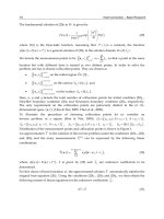
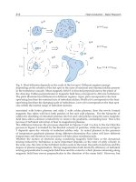
expected to substantially deviate from the physical picture given by the SP solution. Figure 1
demonstrates a simplified version of the physical picture mentioned above with temporal
evolution of the density profile obtained by hydrodynamic simulation for an isothermal
expansion. A spherical target with density and temperature profiles being uniform is
employed as an example. In Fig. 1, the density is always normalized to unity at the center,
and the labels assigned to each curve denote the normalized time /(



), where 

is the
initial radius. The horizontal Lagrange coordinate is normalized to unity at the plasma edge.
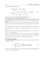
It can be discerned from Fig. 1 that the profile rapidly develops in the early stage for
/(




)≤1. After the rarefaction wave reflects at the center, the density distribution
asymptotically approaches its final self-similar profile (the thick curve with label “  ”),
which is expressed in the Gaussian form, ∝exp[−(/)

] as will be derived below. The
initial and boundary conditions employed in Fig. 1 are substantially simplified such that the
laser-produced shock propagation and resultant interactions with the rarefaction wave are
not described. However, the propagation speeds of the shock and rarefaction waves are
always in the same order as the sound speed 

of the isothermally expanding plasma.
Therefore the physical picture shown in Fig. 1 is expected to be qualitatively valid also for


Fig. 1. Temporal evolution of the density profile of a spherical isothermal plasma, which is
normalized by that at the center; 

and 

are the initial radius and the sound speed,
respectively. After the rarefaction wave reflects at the center, the density distribution
asymptotically approaches its final self-similar profile (the thick curve with “

”).

Heat Conduction – Basic Research

274
realistic cases. Below, we present a self-similar solution for the isothermal expansion of

limited masses (Murakami et al., 2005). The solution explains plasma expansions under
relatively long laser pulses or small-sized targets so that the solution responds to the above
argument on target disintegration. Note that other self-similar solutions of isothermal
plasma expansion have been found for laser-driven two-fluid expansions in light of ion
acceleration physics (Murakami & Basko, 2006) and heavy-ion-driven cylindrical x-ray
converter (Murakami et al., 1990), though they are not discussed here.
2.2 Isothermal expansion
The plasma is assumed to be composed of cold ions and electrons described by one
temperature 

, which is measured in units of energy as follows. Furthermore, the electrons
are assumed to obey the Boltzmann statistics,


=

exp(Φ/

) , (15)
where 

() is the temporal electron density at the target center,  is the elementary charge,
and Φ(,) is the electrostatic potential, the zero-point of which is set at the target center,
i.e., Φ
(
0,
)
=0. The potential Φ satisfies the Poisson equation,

1







Φ

=4
(


−

)
,
(16)

where  is the ionization state; the superscript  stands for the applied geometry such that 
= 1, 2, and 3 correspond to planar, cylinder, and spherical geometry, respectively.
Throughout the present analysis, the electron temperature 

and the ionization state  are
assumed to be constant in space and time.
An ion in the plasma is accelerated via the electrostatic potential in the form,



+



=−



Φ

,
(17)

where 

is the ion mass and  is the ion velocity. Note that, in the following, we consider
such a system that the plasma has quasi-neutrality, i.e., 

≈

, where 

and 

are the
number densities of the ions and the electrons, respectively. Equations (15) and (17) are
combined to derive a single-fluid description,



+



=−




ρ

,
(18)

where 

=



/

is the sound speed. Also, a fluid element with mass density 
(
,
)
=




satisfies the following mass conservation law,




+
1




(



)
=0.
(19)

We now seek a self-similar solution to Eqs. (18) and (19) on (,) and (,) under the
similarity ansatz,

Self-Similar Hydrodynamics with Heat Conduction

275
=

,≡


,
(20)

=







(),
(21)

where () stands for a time-dependent characteristic system size, and  is the
dimensionless similarity coordinate; the over-dot in Eq. (20) denotes the derivative with
respect to time; 

≡(0,0) and 

≡(0) are the initial central density and the size,
respectively; () is a positive unknown function with the normalized boundary condition

(
0
)
=1. Then, Eqs. (15) and (21) give



≈

(


)

(

)
≈











(

)
,
(22)

Under the similarity ansatz, Eqs. (20) and (21), the mass conservation, Eq. (19), is
automatically satisfied. Substituting Eqs. (20) and (21) for Eq. (18), and making use of the
derivative rules, /=

(/) and /=−




(/), one obtains the following
ordinary differential equations in the form of variable separation,






=−



=

,
(23)

where 

(>0) is a separation constant, and the prime denotes the derivative with respect to
. Without losing generality, the constant 

can be set equal to an arbitrary numerical
value, because this is always possible with a proper normalization of R and . Here, just for
simplicity, we set 

=2 in Eq. (23). Then the spatial profile of the density, (), is
straightforwardly obtained under 

(
0
)
=1 in the form (True et al., 1981; London & Rosen,
1986),

(

)
=exp
(
−

)
. (24)
As was seen in Fig. 1, the density profile of isothermally expanding plasma with a limited
mass is found to approach asymptotically the solution, Eq. (24), even if it has a different
profile in the beginning. Meanwhile, () in Eq. (23) cannot be given explicitly as a function
of time but has the following integrated forms,




=2


ln
(
/


)
,

(25)






=
1
2


√
ln
,
/



(26)

where in obtaining Eqs. (25) and (26), the system is assumed to be initially at rest, i.e.,

(
0
)
=

0. Here it should be noted that Eqs. (23) - (26) do not explicitly include the geometrical index
, and therefore they apply to any geometry.
Based on the solution given above, some other important quantities are derived as follows.
First, the total mass of the system 

is conserved and given with the help of Eqs. (21) and
(24) in the form,

Heat Conduction – Basic Research

276


=
(
4
)











exp
(

−

)
=
√







, (27)
with

(
4
)

≡
2,
(
=1
)
2,
(
=2
)
4,
(

=3
)
=
2
/
Γ(/2)
,
(28)

where Γ is the Gamma function. Although the quantitative meaning of () was somewhat
unclear when first introduced in Eq. (20), it can be now clearly understood by relating it to
the temporal central density, 

()≡(0,)≈



()/, with the help of Eqs. (21) and (27)
in the form,


(

)
=
1
√







(

)

/
.
(29)

Additionally the potential Φ and corresponding electrostatic field =−∇Φ are obtained
from Eqs. (15), (21), (22), and (24) in the following forms,

Φ


=−

,
(30)





=
2

.

(31)

The above field quantities contrast well with the fields of the SP solution obtained for a
semi-infinitely stretched planar plasma: Φ/T
e
= −1−/

 and eE/T
e
= 1/c
s
t for
x/c
s
t ≥−1 and >0. It is here worth emphasizing that the electrostatic field increases
linearly with  for the present model, while it is constant in space for the SP model.
Furthermore, the kinetic energy of the system 

() is given with the help of Eqs. (20), (21)
and (27) by



=
(4)

2













exp
(
−

)
=

4





,
(32)

while the internal (thermal) energy of the system 

() is kept constant,




=
3



2

=
3
2





.
(33)

Correspondingly, the power required to keep the isothermal expansion,
(

)
=

/, is
given from Eqs. (23), (25), and (32) in the form,
/

=


ln(/

)/(/

), (34)
where 

=2




/

.
The ion energy spectrum is a physical quantity of high interest. In the present model, the
kinetic energy of an ion in flight directly relates its location, in other words, the further an

Self-Similar Hydrodynamics with Heat Conduction

277
ion is located, the faster it flies. Then, the number of ions contained in an infinitesimally
narrow area of the similarity coordinate between  and + is given by
=(4)









exp
(
−

)
 , (35)
where 

=

/

is the initial number density of the ions at the center. Meanwhile, the
kinetic energy of an ion at  is =






/2, and therefore
=




. (36)

From Eqs. (35) and (36), the ion energy spectrum is obtained,



̂
=
̂
()/
exp(−̂)
Γ(/2)
,
(37)

where 

≡/

and ̂≡/

are normalized quantities with


(

)
=





/2, (38)


=(
√


)



. (39)
It should be noted that, for  = 3, the energy spectrum, Eq. (37), coincides with the well-
known Maxwellian energy distribution; this is not just a coincidence because an
isotropically heated mass always has such a distribution.
Although the spectrum, Eq. (37), is for the ion number density, another spectrum for the
energy density, 

/, is an even more interesting quantity. It can be easily obtained quite
in the same manner as for / taking the specific kinetic energy 

/2into account:



̂
=





Γ(/2)
̂
/
exp
(
−̂
)
.
(40)

The peak value of Eq. (40) is attained at ̂=/2, which is three times higher than that of Eq.
(37) for the spherical case (=3).
2.3 Comparison with experiments
We apply the analytical model to two different laser experiments focusing on the ion energy
spectrum. The two experimental results were separately obtained under different conditions
by means of the time-of-flight method. In both cases, the laser conditions were almost the
same, i.e., the wavelength 

=1.06, the irradiation intensity 

=0.5−1.0×
10

/

, and the pulse length 

~10 with a sufficiently large F-number of a focal
lens. Moreover, the target thicknesses were 


~10. Once the key laser parameters, 

and


, are given, the other basic parameters required for the model analysis are calculated. For
example, the plasma temperature is roughly estimated from the power balance, 



≈
4




(Murakami & Meyer-ter-Vhen, 1991), where 

is the absorption efficiency and 

is
the critical mass density:



[

]
=27(/)

/



/






/
, (41)
where  is the ion mass number. The corresponding sound speed turns out to be in the
order of 10

/, and the disintegration time ~2

/

(recall Fig. 1) is calculated to be

Heat Conduction – Basic Research

278
about 1 ns (≪

~10). The normalized radius /

at the laser turn-off is obtained by Eq.

(26) as a function of the normalized time 

/(

/

). In addition, the scale length of the
plasma expansion is 



~100(≫

~10). Therefore, the present self-similar analysis
is considered to be applicable to the experiments under consideration. From the above key
numerical values, the characteristic ion kinetic energy at the laser turn-off defined by Eq.
(38) is roughly estimated to be 

=2.5−3.5 keV.


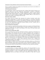
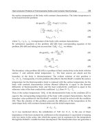
Fig. 2. Comparison of the experimental result (solid line) and the analytical curve (dashed
line) obtained by Eq. (37) under planar geometry. Dotted curves for reference are obtained
by the SP model, Eq. (42).
In the first case, a laser beam was irradiated on a spherical target with diameter of 500,
which was composed of 8-thick plastic shell coated by a 100 nm-thick tin (Sn) layer. In
this case, the plasma expansion during the laser irradiation can be regarded as quasi-planar,
because the plasma scale ~100is appreciably smaller than the laser spot size ~500.
As mentioned in the introduction, the purpose of the Sn-coat was to observe the
characteristics of the EUV light and energetic ion fluxes emitted from the Sn plasma. The

detector was tuned to observe massive Sn ions in the direction of 30 degrees with respect to
the beam axis. Figure 2 shows the ion energy spectrum comparing the experimental result
(solid line) and the analytical curve (dashed line) obtained by Eq. (37) with a fitted
numerical factor 

=1.7 keV and =1 (planar geometry). With respect to the vertical axis,
the physical quantities are properly normalized such that the peak values stay in the order
of unity. The fluctuated structure of the experimental data for >10keV cannot be clearly
judged as concerns whether the signals simply span the region with less precision of
diagnosis, or whether they should be attributed to other causes such as carbon ions, protons,
and photons. In Fig. 2, two other curves (dotted lines) are also plotted for comparison. They
are obtained by the SP model (Mora, 2003),


̂
∝
exp−
√
̂
√
̂
,
(42)

where 

=1.7 keV and 

=0.1 keV are used to draw the fitted curves to relatively low and
high energy regions, respectively. It can be seen that it is hard to reproduce the experimental

Self-Similar Hydrodynamics with Heat Conduction

279
result by Eq. (42). The essential difference of the two analytical models is attributed to their
density profiles, i.e., ∝exp(−

) for the present model and ∝exp(−) for the SP model.
This can be elaborated on as follows: The pressure scale decreases with time all over the
region in the present model, while it is kept constant in time in the SP model. Therefore, the
ions in the former model are less accelerated due to the pdV work than those in the latter
model.


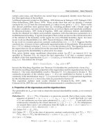
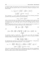
Fig. 3. Comparison of the experimental result (dots) and the analytical curve (dashed line)
obtained by Eq. (37) under spherical geometry.
In the second case, a laser beam was irradiated from a single side with a liquid-Xe jet ejected
through a nozzle with diameter of 30 . The focal spot size was also 30  in diameter.
Therefore, the resultant plasma expansion was very likely unsymmetrical. In this case,
however, the specific mass can expand into much larger space three-dimensionally than in
the first case, and thus is regarded as a quasi-spherical expansion (=3). Figure 3 shows
the experimental result and an analytical curve obtained by Eq. (37) with a fitted numerical
factor 

=3.0 keV. Again, with respect to the vertical axis, the physical quantities are
properly normalized such that the peak values stay in the order of unity. The ion fluxes
were observed at an angle of 45 degrees with respect to the laser beam axis. The
experimental signals strongly fluctuate at energies close to the lowest detection limit at
around ~400eV, but are otherwise well reproduced by the analytical curve.
3. Laser-driven nonstationary accelerating foil due to nonlinear heat

conduction
3.1 Introduction
When one side of a thin planar foil is heated by an external heat source, typically by laser or
thermal x-ray radiation, the heated material quickly expands into vacuum with its density
being reduced drastically - this phenomenon is called “ablation”. In inertial confinement
fusion (ICF) research, for example, it is indispensable to correctly understand the shell
acceleration due to ablation. Thereby self-similar solutions play a crucial role in the analysis
and prediction of the detailed behavior of the shell acceleration. Although some analytical

Heat Conduction – Basic Research

280
models have been proposed to study the shell acceleration due to mass ablation (Gitomer et
al., 1977; Takabe et al., 1983; Kull, 1989, 1991), most of them have assumed a stationary
ablation layer. Pakula and Sigel (1985), for example, reported a self-similar solution for the
ablative heat wave. In the solution, however, the ablation surface is ideally treated such that
the density goes to infinity, and the surface does not accelerate. Below, we present a new
self-similar solution (Murakami et al, 2007), which describes non-stationary acceleration
dynamics of a planar foil target ablatively driven by non-linear heat transfer. The most
striking differences from the other models are that the target has a decreasing mass with a
peak density, and that it has a distinct shell/vacuum boundary, where the density and the
temperature converge to null.
3.2 Basic equations and similarity ansatz
Suppose that a planar shell is being accelerated in the positive direction of the x-axis in an
inertial laboratory frame via the recoil force due to the ablation. The characteristic scale
length of the shell () decreases with time. Let us assume that the shell is burnt out at the
origin of the coordinates, i.e., 
(
0
)

=0 at =0. One can always find such an inertial frame
by appropriately choosing relative position and velocity to another reference inertial frame.
In this case the shell velocity is initially (<0) negative, its absolute value gradually
decreases due to the positive acceleration, and finally the burned-out shell halts at
(
,
)
=
(0,0). The fluid system is then described by the following equations:



+
()

=0,
(43)




+


=−


,
(44)




+


+


=





,
(45)

where  is the mass density,  is the flow velocity,  is the specific internal energy,  is the
temperature in units of energy, and  is the thermal conductivity. We assume an ideal gas
equation of state in the form,
=, =/(−1), (46)
where  is the specific heats ratio. We assume that the thermal conductivity is expressed in
the following power-law form with m, n, and 

being constants,
=




/

. (47)
We introduce the following well-known similarity ansatz (Guderley, 1942; Lie, 1970) to
eliminate the temporal dependence of the system and thus to find a self-similar solution:
=/(), 
(

)
=(−)

, ≥1, (48)
=
(
−
)


(

)
, (49)

Self-Similar Hydrodynamics with Heat Conduction

281
=
(


)

(
−
)

(

)

(

)
, (50)

=
(
−
)


(

)
,=
2
(
−1
)(
−1

)
−1
1+
,
(51)

where  is the self-similar variable; (), (), and () stand for the self-similar profiles of
the velocity, temperature, and density, respectively; ,  and  are arbitrary constants. In
most of numerical calculations in this paper, we employ =2 (constant acceleration),
(,)=(0,5/2) (electron heat conductivity) and =5/3 as a reference case. The constraint,
≥1, in Eq. (48) stems from Eqs. (49) and (50) in order that  and  do not diverge to
infinity as →0. The limiting value, =1, corresponds to a special case, where the
characteristic scale of  and  are kept constant in time, while =(2−1)/2(−1)=4/3
corresponds to another special case, where the density scale does not change in time, i.e.,
=0 [see Eq. (51)].
Using ansatz (48) - (51), Eqs. (43) - (45) are reduced to the following set of ordinary
differential equations:

(
+
)


+

−


=0,
(52)

(+)′+(

−1)+()′/=0, (53)
(−1)

[
(+)′+2(

−1)
]
+′=

(





)′ (54)
where the prime denotes the derivative with respect to , and
=







(55)

is a dimensionless parameter. Solving Eqs. (52) and (53) algebraically for ′ and ′, one finds
that a singular point appears when +=±
√

(more details on the singular point will be
given later). Let 

, 

, 

, and 

be their values at the singular point. Here we introduce re-
normalized variables, ξ, U(ξ), G(ξ), and Θ(ξ):

=
−




,=
−




,=




,=



,
(56)

At the singular point, =0, the re-normalized variables are specified to be

(
0
)
=−1,
(
0
)
=1,
(
0
)
=1, (57)
where we employ the flow direction such that 

+

=−




. Equations (10) - (12) are then
transformed to
(+)′+(′−/)=0, (58)
(+)′+(

−1)+()′/+

=0, (59)
(−1)

[
(+)′+2(

−1)
]
+′=



(





)′ (60)
where the prime hereafter denotes the derivative with respect to , and

Heat Conduction – Basic Research

282


=
(
1−

)


/



, 

=





, (61)
are dimensionless constants representing the gravity (acceleration) and the heat
conductivity, respectively. Thus the system is clearly defined by Eqs. (57) - (60). Equations
(58) and (59) yield




=




, 

=


−
(
+
)




,
(62)

where


=(+)

−, (63)




=



(
+
)
+
(


−1
)
+

+

.
(64)

It is clear that G′ and U′ in Eq. (62) are singular when 

=0. This singular point corresponds
to the sonic point, where the flow velocity relative to the surface = is equal to the
local isothermal sound speed. An integrated curve which is physically acceptable is
expected to pass this singular sonic point smoothly, the condition of which is given by


=


=0. (65)
Since =0 is the singular point, one should start numerical integration at its infinitesimally
adjacent point. One then needs the four derivatives ′(0), ′(0), ′(0), and ′′(0), which are
fully provided by relation (65). At =0, the derivatives of Eq. (62) are reduced from
L'Hopital's theorem to



=






,

=


+






.
(66)

Thus all the four derivatives at the sonic point are explicitly obtained from Eqs. (57) - (60),
and (66).
The present system has another singular point at the vacuum interface, the coordinate at
which, =

, is an eigenvalue of the system. On the vacuum interface the relative flow
velocity to the free surface vanishes, i.e., (

)+

=0, which can also be interpreted as the
definition of the free surface. Moreover at =

the pressure and thus the density are
expected to vanish coherently, because practically no heat conduction prevails in this front
region (typically characterized such that ≫1, ≪1, and
(
+
)

≪Θ) and thus the
specific entropy is kept constant in time. It is then shown that Eqs. (16) and (18) (neglecting
the heat conduction) have the adiabatic integral with an arbitrary constant 

(Zel’dovich &
Raizer, 1966):

(+)




=

,≡
2
(
1−
)
+
(
−1
)
+
.
(67)

The vacuum interface is a singular point of the adiabatic flow of the saddle type (Sanz et al.,
1988), where the spatial profiles in the vicinity of =

is worked out from Eqs. (58) - (60) to
a first-order approximation in (

−):

Self-Similar Hydrodynamics with Heat Conduction

283
≈

(

+1
)
−2
(


+
(
−1
)


)
(
+
)

(


−
)
,
(68)


+≈−
+1−2



(


−
)

(69)


≈

(


−
)

,≡
−++2

(
+1
)
−2
,
(70)

where 

is an arbitrary constant; 


≈

(

−

)

for a relatively high aspect shell, i.e.,


/(

−

)≫1, where 

and 

are their corresponding values at the density peak; 


and 

are also eigenvalues of the system as will be given below together with 

. In
particular, under constant acceleration (=2), the velocity becomes constant, =−


, and
∝(

−

) apart from a linear temperature profile in space, as one can predict from Eqs.
(69) and (70).


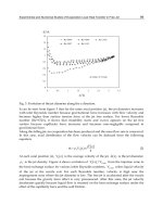
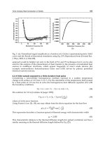
Fig. 4. Eigenstructure of the accelerated shell under a constant gravity (=2).
3.3 Two dimensional eigenvalue problem and numerical results
Although one can start the numerical integration at =0 toward the positive direction of -
axis, it soon turns out that such numerical integrations produce physically unacceptable
pictures under an arbitrary set of the values of 

and 

such that →∞ on its way in the
integration without showing the converging behavior, Eqs. (68) - (70), at the vacuum
boundary. Therefore the present system is supposed to be an eigenvalue problem, in which
only some special combinations of 

and 

can produce the converging behavior expected
as a physically meaningful solution (Murakami et al., 2004).
Figure 4 shows such an eigenstructure numerically obtained for the density , the
temperature Θ, the velocity , and the pressure =Θ under the fixed parameters given in
Fig. 4. As mentioned earlier, the spatial profiles thus obtained strikingly contrast with ones
for the stationary ablation models (Gitomer et al., 1977; Takabe et al., 1983; Kull, 1989, 1991).

Heat Conduction – Basic Research

284

Fig. 5. Magnified view of Fig.4 around the ablation surface.
Figure 5 shows the magnified view around the ablation surface of Fig. 4, in which the mass
flux relative to the surface with =, ≡−(+), is additionally depicted.
Surprisingly the predicted profiles, (68) - (70), apply not only to the vicinity of the vacuum
boundary but also to almost all the region beyond the ablation surface (>0.1763). This in
turn supports the earlier argument that the heat conduction in the shell is practically
negligible. It should also be noted that at =

the physical quantities seemingly have a
sharp jump in their derivatives. However, all those quantities change smoothly but on a
very narrow range, which can be observed in the further magnified view for  in the upper
right corner in Fig. 5. The characteristic scale length of the drastic change in the physical
quantities can be roughly estimated from Eq. (60) to be Δ

~Θ


/|

|


~(10

) as

can be observed in Fig. 5.
4. Gravitational collapse of radiatively cooling sphere in view of star-
formation
4.1 Introduction
Self-similar solutions play a crucial role in astrophysics as well. Below we describe a
spherically contracting system observed in the star formation processes, in which the effect
of radiative heart conduction is expected to play an important role. In such a system,
substantial dissociation and ionization of molecules and atoms proceed with time, and the
isothermal assumption used in the so-called LP model (Larson, 1969; Penston, 1969)
becomes inappropriate. A solution introduced here (Murakami et al., 2004) can be clearly
placed in a thermodynamic perspective as follows: The LP model with the isothermal
assumption means infinitely large heat conductivity, i.e., →0, where  denotes the
P́clet number. Meanwhile, there are a number of works based on the perfect adiabaticity,
i.e., →∞, which corresponds to zero heat conductivity (Sedov, 1959; Barenblatt, 1979;
Antonova, 2000). These are two opposed limiting cases, with which the analytical and
numerical treatment are substantially simplified, and the energy conservation law is often
expressed in an integrated form or neatly installed in the equation of motion. In contrast, we
explicitly leave the radiative conduction term in the hydrodynamic system to handle its
nonlinear effect.

Self-Similar Hydrodynamics with Heat Conduction

285
An important feature of the present subsection, which is essentially different from the
conventional ones obtained under the isothermal or adiabatic assumptions, is that all the
scales of the physical quantities are uniquely determined as a function of time only. This is
clear from the following argument: When discussing self-similarity within the one-
dimensional framework, one needs four physical quantities to produce a dimensionless
parameter as a basic self-similar variable, where the system is contained in the class of
systems of the so-called MLT fundamental units of measurement. Radius r, time t, and the

gravitational constant G, are apparently the first three quantities in a spherically contracting
system under self-gravity. The fourth quantity is, for example, the temperature for an
isothermal system, or the specific entropy for an adiabatic system. Such quantities cannot be
specified in the absolute value, and therefore they can serve as an external control parameter
of individual systems. In the present system, however, the fourth quantity is the heat
diffusion conductivity, 

; the numerical value of which is quite unique, once the conductive
mechanism is specified. Therefore 

can never be a control parameter, and the resultant
behavior of the system is unique.
4.2 Basic equation and similarity ansatz
The one-dimensional spherical gas-dynamical equations with both self-gravity and
diffusivity are



+
1




(



)
=0,

(71)




+


=−
1



−


,
(72)


1








=4,

(73)





+


+





(



)
=
1











(74)

where p is the pressure,  the density,  the specific internal energy, u the flow velocity, and
 the gravitational potential. We assume the ideal gas equation of state (EOS) in the form,

(
+1
)



=


=
(
−1
)
,
(75)

where k
B
is the Boltzmann constant,  the mean atomic mass, and  the specific heats ratio; Z
is the ionization state, and =1 is assumed for hydrogen plasma. Equation (74), described
by the one-temperature model, includes the non-linear heat diffusion term on the right hand
side, where we assume a power-law dependence for the diffusion coefficient, =




/

,
with 

, m, and n being constants. For normal physical values, >0 and >0 are
assumed. With an intention to apply our solution primarily to the case of radiative heat
diffusion, we can express  as =(16



)/3

where
3
0
/



mn
R
T
is the Rosseland

Heat Conduction – Basic Research

286

mean opacity, 

is the Stefan-Boltzmann constant, and 

=16

/3

is a constant. In the
formulae given below, we keep the generality in terms of the parameters, m, n, and , but
also show specific forms using the values of the reference set at the same time: =2,
=13/2, and 

describing the opacity due to inverse bremsstrahlung in a fully ionized
hydrogen plasma (Zel'dovich & Raizer, 1966) together with =5/3.
To find a self-similar solution, we here introduce the following group transformation,
=̂, =

,

=

, =



, =

, =




(76)
where the hats denote the physical quantities in the scaled system related by the scale factor
 with the parent system without hats. The constants, a, b, c, d, and e, can be appropriately
determined by substituting Eq. (76) for Eqs. (71) - (74) such that the transformed system is
kept symmetric and thus has the same structure as the original one based on the Lie's idea
(Lie, 1970):
1−==/2=1+/2=/2=(1∗2)/(3+2−2). (77)
For the reference case, m = 2 and n = 13/2, Eq. (77) gives =11/6, =−5/6, ==−5/3,
and =−11/3. Equation (77), together with the following similarity ansatz, enables the
removal of the temporal dependence from Eqs. (71) - (74),

(

)
=
|

|
/
, ≡r/R(t), (78)

=


|

|
/

(),
(79)


=




|

|
/

(

)
,
(80)

=
|

|

(), (81)



=




|

|
()/
Ω
(

)
,Ω()≡4
(

)
,



(82)

where 
(

)
is the temporal characteristic scale length of the system; A and B are positive
constants defining the scales of the radius and the density, respectively. Note that the
relation, /=−2, is used for the similarity ansatz of the density in Eq. (84), which holds
regardless of the values of m and n. Furthermore, it should be noted that, at a glance, the
ansatz for u and T given in Eqs. (82) and (83) seem to be bounded with each other with the

similar front factors, / and (/)
2
, respectively. However, these factors are chosen just for
simplicity, and u and T are kept independent of each other, because the functions, () and

(

)
, are left free until they are self-consistently determined as the solution of the eigenvalue
problem as shown below. In this paper, we consider a contracting fluid system for <0
which collapses at =0, and therefore ||=−. Then, Eqs. (71), (72), and (74) are
respectively reduced to the following ordinary differential equations,

Self-Similar Hydrodynamics with Heat Conduction

287
−
(
±−
)


+±+

+


=0, (83)

±−

(
±−
)


+
(

)


+


Ω


=0,
(84)


±−(±−)

−1
+

+
2

=


(







)



,
(85)

where the prime denotes the derivative with respect to , and concerning the double signs,
(
±
)
, the upper (plus) and lower (minus) sign correspond to >0 and <0, respectively.
Since Eq. (73) is automatically satisfied, its reduced form does not appear in the above set of
equations. Thus, the present system is characterized by the two positive dimensionless
parameters, 

and 

, defined by 

=


 and 

=(

/

)(/)

. It can be
interpreted that 

and K
2
are introduced for simplicity instead of A and B. Equations (83) -
(85) are second-order ordinary equation system for , , and , and the obvious boundary
conditions are

(
0
)
=0, 
(
0
)
=1, (0)=1, ()


=0. (86)
The last relation means that there is no pressure gradient at the center.

4.3 The self-similar solution as two dimensional eigenvalue problem
At first glance, the ODE system, Eqs. (83) - (85), together with the boundary condition (86),
seem to be closed mathematically. However, one can easily find that numerical integration
of the system produces a physically unacceptable picture under an arbitrary set of the
values for 

and 

such that the temperature suddenly diverges to infinity at a finite
radius. Since the physical quantities are expected to change smoothly in space, it is
conjectured that some special values of 

and 

, which are still unknown, can give such a
physically acceptable picture. Therefore the present system is supposed to be a two-
dimensional eigenvalue problem, which is essentially different from the one-dimensional
eigenvalue problems of the previous work.
To determine a unique set of parameters, 

and 

, we need two more physical conditions.
The first one is quite an orthodox prescription, in which the right integration curve
smoothly passes through the singular point, which is located somewhere at a finite distance
from the center. On this singular point, the fluid velocity is equal to the local sound speed.
The second parameter is less obvious compared with the first one, but still seems natural
enough, namely, that both the density and the temperature converge to zero simultaneously
with an increase in radius. The numerical calculation is started from the center, and
therefore it is necessary to make clear the asymptotic behavior of the solution in the vicinity

of the center as follows.
For the central region, the asymptotic behaviors of the above physical quantities are
obtained by inserting the following ansatz,
=1−



, =1−



, =−

,
(
≪1
)
, (87)

Heat Conduction – Basic Research

288
into Eqs. (83) - (85), where 

, 

, and 

are unknown positive constants, where we make
use of the symmetry at the center and thus employed only the lowest quadratic terms for 

and . After some manipulation, the constants are obtained,



=
2(−1)
3(−−3/2)
,

=
(
−1
)
−−+1/2
3
(
−1
)(
−−3/2
)




=2

−






4

(88)

As can be seen in Eq. (88), in order to conduct the numerical calculation starting from the
center, 

and 

must both be specified as trial values, which are expected to converge to
their genuine eigenvalues after numerical iteration. Figure 6 shows the first step of the
solving process, or how a right eigenvalue, 

, is obtained on the - plane, where 

=0.64
is fixed just as a trial value. As can be seen in Figure 6, there exists an appropriate value of


, with which the integrated curve smoothly passes through the singular point, while the
other integrated curves deviate from the right curve as the integration proceeds toward the
singular point, resulting in an unacceptable physical picture. In this manner, an appropriate
eigenvalue 

can be determined as a function of arbitrary 

.

Fig. 6. g -  diagram showing the optimization process of the eigenvalue, 

.
Under the condition that the right integrated curve is to smoothly pass through a singular
point, the integrations are conducted from the center (==1) with the radius toward
infinity corresponding to ==0. Fixed parameters are =2, =13/2, =5/3, and


=0.64. As the second step, one needs to determine 

that satisfies the second
requirement mentioned earlier, namely, →0 and →0 at the same time. Figure 7 shows
how the right eigenvalue, 

, is determined on the - plane, where each curve is already
optimized such that it passes through each singular point. As a result, it turns out that there
exists a unique pair of the eigenvalues of 

and 

, which satisfies the both requirements.
Figure 8 shows the eigenstructure for the temperature, ∝ the density, ∝, the velocity,
∝, and the heat flux, ∝−∇, under the eigenvalues of the reference system thus
obtained, where the curves are assigned with labels corresponding to the original physical