Sensor Fusion and its Applications Part 2 pdf
Bạn đang xem bản rút gọn của tài liệu. Xem và tải ngay bản đầy đủ của tài liệu tại đây (973.46 KB, 30 trang )
Sensor Fusion and Its Applications24
1,1 1, 1,
,1 , ,
,1 , ,
T
1,1
1
1
,
,
( 1) ( 1) ( 1)
( 1) ( 1) ( 1)
( 1) ( 1) ( 1)
( ) 0 0
( 1) 0 0
( 1) 0
0 ( ) 0
0 ( 1) 0
0 0 ( )
0 0 ( )
N m
N N N N m
m m N mm
N N
N
mm
k k k
k k k
k k k
k
k
k
k
k
k
k
P P P
P P P
P P P
P
B
B
P
B
P
Φ
T
T
1
T
1
1
1
1
T
1
T
0
0 ( 1) 0
0 0 ( )
( 1) 0 0
( ) 0 0
( 1) 0 0
0 ( 1) 0
0 ( ) 0
0 ( 1) 0
0 0 ( )
0 0 ( )
0 0 ( )
N
N
N
N
m
k
k
k
k
k
k
k
k
k
k
k
B
Φ
C
Q
C
C
Q
C
Γ
Q
Γ
(4.14)
If taken the equal sign, that is, achieved the de-correlation of local estimates, on the one
hand, the global optimal fusion estimate can be realized by Theorem 4.1 , but on the other,
the initial covariance matrix and process noise covariance of the sub-filter themselves can
enlarged by
1
i
times. What’s more, the filter results of every local filter will not be
optimal.
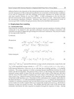
4.2 Structure and Performance Analysis of the Combined Filter
The combined filter is a 2-level filter. The characteristic to distinguish from the traditional
distributed filters is the use of information distribution to realize information share of every
sub-filter. Information fusion structure of the combined filter is shown in Fig. 4.1.
公共基准系统
子系统 1
子系统 2
子系统 N
子滤波器 1
子滤波器 2
子滤波器 N
主滤波器
时间更新
最优融合
1
1
ˆ
,
g
g
X
P
1 1
ˆ
,
X
P
1
2
ˆ
,
g
g
X
P
ˆ
,
N
N
X
P
2 2
ˆ
,
X
P
1
ˆ
,
g
N g
X
P
ˆ
,
m m
X
P
ˆ
,
g
g
X
P
ˆ
,
g
g
X
P
1
m
1
Z
2
Z
N
Z
Sub-filter 2
Sub-system 1
Sub-system N
Sub-system 2
Public reference
Sub-filter N
Sub-filter 1
Sub-filter 2
Updated time
Master Filter
Optimal fusion
Fig. 4.1 Structure Indication of the Combined Filter
From the filter structure shown in the Fig. 4.1, the fusion process for the combined filter can
be divided into the following four steps.
Step1 Given initial value and information distribution: The initial value of the global state in
the initial moment is supposed to be
0
X
, the covariance to be
0
Q , the state estimate vector
of the local filter, the system covariance matrix and the state vector covariance matrix
separately, respectively to be
ˆ
, , , 1, ,
i i i
i NX Q P
, and the corresponding master filter
to be
ˆ
, ,
m m m
X
Q P
.The information is distributed through the information distribution
factor by the following rules in the sub-filter and the master filter.
1 1 1 1 1 1 1
1 2
1 1 1 1 1 1 1
1 2
( ) ( ) ( ) ( ) ( ) ( ) ( )
( | ) ( | ) ( | ) ( | ) ( | ) ( | ) ( | )
ˆ ˆ
( | ) ( | ) 1,2, , ,
g N m i i g
g N m i i g
i g
k k k k k k k
k k k k k k k k k k k k k k
k k k k i N m
Q Q Q Q Q Q Q
P P P P P P P
X X
(4.15)
Where,
i
should meet the requirements of information conservation principles:
1 2
1 0 1
N m i
Step2 the time to update the information: The process of updating time conducted
independently, the updated time algorithm is shown as follows:
T T
ˆ ˆ
( 1| ) ( 1| ) ( | ) 1, 2, , ,
( 1| ) ( 1| ) ( | ) ( 1| ) ( 1| ) ( ) ( 1| )
i i
i i i
k k k k k k i N m
k k k k k k k k k k k k k
X Φ X
P Φ P Φ Γ Q Γ
(4.16)
Step3 Measurement update: As the master filter does not measure, there is no measurement
update in the Master Filter. The measurement update only occurs in each local sub-filter,
and can work by the following formula:
1 1 T 1
1 1 T 1
ˆ ˆ
( 1| 1) ( 1| 1) ( 1| ) ( 1| ) ( 1) ( 1) ( 1)
( 1| 1) ( 1| ) ( 1) ( 1) ( 1) 1,2, ,
i i i i i i i
i i i i i
k k k k k k k k k k k
k k k k k k k i N
P X P X H R Z
P P H R H
(4.17)
Step4 the optimal information fusion: The amount of information of the state equation and
the amount of information of the process equation can be apportioned by the information
distribution to eliminate the correlation among sub-filters. Then the core algorithm of the
combined filter can be fused to the local information of every local filter to get the state
optimal estimates.
,
1
1
,
1 1 1 1 1 1 1
1 2
1
ˆ ˆ
( | ) ( | ) ( | ) ( | )
( | ) ( ( | )) ( ( | ) ( | ) ( | ) ( | ))
N m
g g i i
i
N m
g i N m
i
k k k k k k k k
k k k k k k k k k k k k
X P P X
P P P P P P
(4.18)
It can achieve the goal to complete the workflow of the combined filter after the processes of
information distribution, the updated time, the updated measurement and information
fusion. Obviously, as the variance upper-bound technique is adopted to remove the
State Optimal Estimation for Nonstandard Multi-sensor Information Fusion System 25
1,1 1, 1,
,1 , ,
,1 , ,
T
1,1
1
1
,
,
( 1) ( 1) ( 1)
( 1) ( 1) ( 1)
( 1) ( 1) ( 1)
( ) 0 0
( 1) 0 0
( 1) 0
0 ( ) 0
0 ( 1) 0
0 0 ( )
0 0 ( )
N m
N N N N m
m m N mm
N N
N
mm
k k k
k k k
k k k
k
k
k
k
k
k
k
P P P
P P P
P P P
P
B
B
P
B
P
Φ
T
T
1
T
1
1
1
1
T
1
T
0
0 ( 1) 0
0 0 ( )
( 1) 0 0
( ) 0 0
( 1) 0 0
0 ( 1) 0
0 ( ) 0
0 ( 1) 0
0 0 ( )
0 0 ( )
0 0 ( )
N
N
N
N
m
k
k
k
k
k
k
k
k
k
k
k
B
Φ
C
Q
C
C
Q
C
Γ
Q
Γ
(4.14)
If taken the equal sign, that is, achieved the de-correlation of local estimates, on the one
hand, the global optimal fusion estimate can be realized by Theorem 4.1 , but on the other,
the initial covariance matrix and process noise covariance of the sub-filter themselves can
enlarged by
1
i
times. What’s more, the filter results of every local filter will not be
optimal.
4.2 Structure and Performance Analysis of the Combined Filter
The combined filter is a 2-level filter. The characteristic to distinguish from the traditional
distributed filters is the use of information distribution to realize information share of every
sub-filter. Information fusion structure of the combined filter is shown in Fig. 4.1.
公共基准系统
子系统 1
子系统 2
子系统 N
子滤波器 1
子滤波器 2
子滤波器 N
主滤波器
时间更新
最优融合
1
1
ˆ
,
g
g
X
P
1 1
ˆ
,
X
P
1
2
ˆ
,
g
g
X
P
ˆ
,
N
N
X
P
2 2
ˆ
,
X
P
1
ˆ
,
g
N g
X
P
ˆ
,
m m
X
P
ˆ
,
g
g
X
P
ˆ
,
g
g
X
P
1
m
1
Z
2
Z
N
Z
Sub-filter 2
Sub-system 1
Sub-system N
Sub-system 2
Public reference
Sub-filter N
Sub-filter 1
Sub-filter 2
Updated time
Master Filter
Optimal fusion
Fig. 4.1 Structure Indication of the Combined Filter
From the filter structure shown in the Fig. 4.1, the fusion process for the combined filter can
be divided into the following four steps.
Step1 Given initial value and information distribution: The initial value of the global state in
the initial moment is supposed to be
0
X
, the covariance to be
0
Q , the state estimate vector
of the local filter, the system covariance matrix and the state vector covariance matrix
separately, respectively to be
ˆ
, , , 1, ,
i i i
i NX Q P
, and the corresponding master filter
to be
ˆ
, ,
m m m
X
Q P
.The information is distributed through the information distribution
factor by the following rules in the sub-filter and the master filter.
1 1 1 1 1 1 1
1 2
1 1 1 1 1 1 1
1 2
( ) ( ) ( ) ( ) ( ) ( ) ( )
( | ) ( | ) ( | ) ( | ) ( | ) ( | ) ( | )
ˆ ˆ
( | ) ( | ) 1,2, , ,
g N m i i g
g N m i i g
i g
k k k k k k k
k k k k k k k k k k k k k k
k k k k i N m
Q Q Q Q Q Q Q
P P P P P P P
X X
(4.15)
Where,
i
should meet the requirements of information conservation principles:
1 2
1 0 1
N m i
Step2 the time to update the information: The process of updating time conducted
independently, the updated time algorithm is shown as follows:
T T
ˆ ˆ
( 1| ) ( 1| ) ( | ) 1, 2, , ,
( 1| ) ( 1| ) ( | ) ( 1| ) ( 1| ) ( ) ( 1| )
i i
i i i
k k k k k k i N m
k k k k k k k k k k k k k
X Φ X
P Φ P Φ Γ Q Γ
(4.16)
Step3 Measurement update: As the master filter does not measure, there is no measurement
update in the Master Filter. The measurement update only occurs in each local sub-filter,
and can work by the following formula:
1 1 T 1
1 1 T 1
ˆ ˆ
( 1| 1) ( 1| 1) ( 1| ) ( 1| ) ( 1) ( 1) ( 1)
( 1| 1) ( 1| ) ( 1) ( 1) ( 1) 1,2, ,
i i i i i i i
i i i i i
k k k k k k k k k k k
k k k k k k k i N
P X P X H R Z
P P H R H
(4.17)
Step4 the optimal information fusion: The amount of information of the state equation and
the amount of information of the process equation can be apportioned by the information
distribution to eliminate the correlation among sub-filters. Then the core algorithm of the
combined filter can be fused to the local information of every local filter to get the state
optimal estimates.
,
1
1
,
1 1 1 1 1 1 1
1 2
1
ˆ ˆ
( | ) ( | ) ( | ) ( | )
( | ) ( ( | )) ( ( | ) ( | ) ( | ) ( | ))
N m
g g i i
i
N m
g i N m
i
k k k k k k k k
k k k k k k k k k k k k
X P P X
P P P P P P
(4.18)
It can achieve the goal to complete the workflow of the combined filter after the processes of
information distribution, the updated time, the updated measurement and information
fusion. Obviously, as the variance upper-bound technique is adopted to remove the
Sensor Fusion and Its Applications26
correlation between sub-filters and the master filter and between the various sub-filters in
the local filter and to enlarge the initial covariance matrix and the process noise covariance
of each sub-filter by
1
i
times, the filter results of each local filter will not be optimal. But
some information lost by the variance upper-bound technique can be re-synthesized in the
final fusion process to get the global optimal solution for the equation.
In the above analysis for the structure of state fusion estimation, it is known that centralized
fusion structure is the optimal fusion estimation for the
system state in the minimum
variance. While in the combined filter, the optimal fusion algorithm is used to deal with
local filtering estimate to synthesize global state estimate. Due to the application of variance
upper-bound technique, local filtering is turned into being suboptimal, the global filter after
its synthesis becomes global optimal, i.e. the fact that the equivalence issue between the
combined filtering process and the centralized fusion filtering process. To sum up, as can be
seen from the above analysis, the algorithm of combined filtering process is greatly
simplified by the use of variance upper-bound technique. It is worth pointing out that the
use of variance upper-bound technique made local estimates suboptimum but the global
estimate after the fusion of local estimates is optimal, i.e. combined filtering model is
equivalent to centralized filtering model in the estimated accuracy.
4.3 Adaptive Determination of Information Distribution Factor
By the analysis of the estimation performance of combined filter, it is known that the
information distribution principle not only eliminates the correlation between sub-filters as
brought from public baseline information to make the filtering of every sub-filter conducted
themselves independently, but also makes global estimates of information fusion optimal.
This is also the key technology of the fusion algorithm of combined filter. Despite it is in this
case, different information distribution principles can be guaranteed to obtain different
structures and different characteristics (fault-tolerance, precision and amount of calculation)
of combined filter. Therefore, there have been many research literatures on the selection of
information distribution factor of combined filter in recent years. In the traditional structure
of the combined filter, when distributed information to the subsystem, their distribution
factors are predetermined and kept unchanged to make it difficult to reflect the dynamic
nature of subsystem for information fusion. Therefore, it will be the main objective and
research direction to find and design the principle of information distribution which will be
simple, effective and dynamic fitness, and practical. Its aim is that the overall performance
of the combined filter will keep close to the optimal performance of the local system in the
filtering process, namely, a large information distribution factors can be existed in high
precision sub-system, while smaller factors existed in lower precision sub-system to get
smaller to reduce its overall accuracy of estimated loss. Method for determining adaptive
information allocation factors can better reflect the diversification of estimation accuracy in
subsystem and reduce the impact of the subsystem failure or precision degradation but
improve the overall estimation accuracy and the adaptability and fault tolerance of the
whole system. But it held contradictory views given in Literature [28] to determine
information distribution factor formula as the above held view. It argued that global optimal
estimation accuracy had nothing to do with the information distribution factor values when
statistical characteristics of noise are known, so there is no need for adaptive determination.
Combined with above findings in the literature, on determining rules for information
distribution factor, we should consider from two aspects.
1) Under circumstances of meeting conditions required in Kalman filtering such as exact
statistical properties of noise, it is known from filter performance analysis in Section 4.2 that:
if the value of the information distribution factor can satisfy information on conservation
principles, the combined filter will be the global optimal one. In other words, the global
optimal estimation accuracy is unrelated to the value of information distribution factors,
which will influence estimation accuracy of a sub-filter yet. As is known in the information
distribution process, process information obtained from each sub-filter is
1 1
,
i g i g
Q P
,
Kalman filter can automatically use different weights according to the merits of the quality
of information: the smaller the value of
i
is, the lower process message weight will be, so
the accuracy of sub-filters is dependent on the accuracy of measuring information; on the
contrary, the accuracy of sub-filters is dependent on the accuracy of process information.
2) Under circumstances of not knowing statistical properties of noise or the failure of a
subsystem, global estimates obviously loss the optimality and degrade the accuracy, and it
is necessary to introduce the determination mode of adaptive information distribution factor.
Information distribution factor will be adaptive dynamically determined by the sub-filter
accuracy to overcome the loss of accuracy caused by fault subsystem to remain the relatively
high accuracy in global estimates. In determining adaptive information distribution factor, it
should be considered that less precision sub-filter will allocate factor with smaller
information to make the overall output of the combined filtering model had better fusion
performance, or to obtain higher estimation accuracy and fault tolerance.
In Kalman filter, the trace of error covariance matrix
P
includes the corresponding estimate
vector or its linear combination of variance. The estimated accuracy can be reflected in filter
answered to the estimate vector or its linear combination through the analysis for the trace
of
P. So there will be the following definition:
Definition 4.1: The estimation accuracy of attenuation factor of the
i
th local filter is:
T
tr( )
i i i
EDOP
P
P
(4.19)
Where, the definition of
i
E
DOP
(Estimation Dilution of Precision) is attenuation factor
estimation accuracy, meaning the measurement of estimation error covariance matrix
in
i
local filter
,
tr( )
meaning the demand for computing trace function of the matrix.
When introduced attenuation factor estimation accuracy
i
E
DOP , in fact, it is said to use
the measurement of norm characterization
i
P in
i
P
matrix: the bigger the matrix norm is,
the corresponding estimated covariance matrix will be larger, so the filtering effect is poorer;
and vice versa.
According to the definition of attenuation factor estimation accuracy, take the computing
formula of information distribution factor in the combined filtering process as follows:
1 2
i
i
N m
EDOP
E
DOP EDOP EDOP EDOP
(4.20)
State Optimal Estimation for Nonstandard Multi-sensor Information Fusion System 27
correlation between sub-filters and the master filter and between the various sub-filters in
the local filter and to enlarge the initial covariance matrix and the process noise covariance
of each sub-filter by
1
i
times, the filter results of each local filter will not be optimal. But
some information lost by the variance upper-bound technique can be re-synthesized in the
final fusion process to get the global optimal solution for the equation.
In the above analysis for the structure of state fusion estimation, it is known that centralized
fusion structure is the optimal fusion estimation for the
system state in the minimum
variance. While in the combined filter, the optimal fusion algorithm is used to deal with
local filtering estimate to synthesize global state estimate. Due to the application of variance
upper-bound technique, local filtering is turned into being suboptimal, the global filter after
its synthesis becomes global optimal, i.e. the fact that the equivalence issue between the
combined filtering process and the centralized fusion filtering process. To sum up, as can be
seen from the above analysis, the algorithm of combined filtering process is greatly
simplified by the use of variance upper-bound technique. It is worth pointing out that the
use of variance upper-bound technique made local estimates suboptimum but the global
estimate after the fusion of local estimates is optimal, i.e. combined filtering model is
equivalent to centralized filtering model in the estimated accuracy.
4.3 Adaptive Determination of Information Distribution Factor
By the analysis of the estimation performance of combined filter, it is known that the
information distribution principle not only eliminates the correlation between sub-filters as
brought from public baseline information to make the filtering of every sub-filter conducted
themselves independently, but also makes global estimates of information fusion optimal.
This is also the key technology of the fusion algorithm of combined filter. Despite it is in this
case, different information distribution principles can be guaranteed to obtain different
structures and different characteristics (fault-tolerance, precision and amount of calculation)
of combined filter. Therefore, there have been many research literatures on the selection of
information distribution factor of combined filter in recent years. In the traditional structure
of the combined filter, when distributed information to the subsystem, their distribution
factors are predetermined and kept unchanged to make it difficult to reflect the dynamic
nature of subsystem for information fusion. Therefore, it will be the main objective and
research direction to find and design the principle of information distribution which will be
simple, effective and dynamic fitness, and practical. Its aim is that the overall performance
of the combined filter will keep close to the optimal performance of the local system in the
filtering process, namely, a large information distribution factors can be existed in high
precision sub-system, while smaller factors existed in lower precision sub-system to get
smaller to reduce its overall accuracy of estimated loss. Method for determining adaptive
information allocation factors can better reflect the diversification of estimation accuracy in
subsystem and reduce the impact of the subsystem failure or precision degradation but
improve the overall estimation accuracy and the adaptability and fault tolerance of the
whole system. But it held contradictory views given in Literature [28] to determine
information distribution factor formula as the above held view. It argued that global optimal
estimation accuracy had nothing to do with the information distribution factor values when
statistical characteristics of noise are known, so there is no need for adaptive determination.
Combined with above findings in the literature, on determining rules for information
distribution factor, we should consider from two aspects.
1) Under circumstances of meeting conditions required in Kalman filtering such as exact
statistical properties of noise, it is known from filter performance analysis in Section 4.2 that:
if the value of the information distribution factor can satisfy information on conservation
principles, the combined filter will be the global optimal one. In other words, the global
optimal estimation accuracy is unrelated to the value of information distribution factors,
which will influence estimation accuracy of a sub-filter yet. As is known in the information
distribution process, process information obtained from each sub-filter is
1 1
,
i g i g
Q P
,
Kalman filter can automatically use different weights according to the merits of the quality
of information: the smaller the value of
i
is, the lower process message weight will be, so
the accuracy of sub-filters is dependent on the accuracy of measuring information; on the
contrary, the accuracy of sub-filters is dependent on the accuracy of process information.
2) Under circumstances of not knowing statistical properties of noise or the failure of a
subsystem, global estimates obviously loss the optimality and degrade the accuracy, and it
is necessary to introduce the determination mode of adaptive information distribution factor.
Information distribution factor will be adaptive dynamically determined by the sub-filter
accuracy to overcome the loss of accuracy caused by fault subsystem to remain the relatively
high accuracy in global estimates. In determining adaptive information distribution factor, it
should be considered that less precision sub-filter will allocate factor with smaller
information to make the overall output of the combined filtering model had better fusion
performance, or to obtain higher estimation accuracy and fault tolerance.
In Kalman filter, the trace of error covariance matrix
P
includes the corresponding estimate
vector or its linear combination of variance. The estimated accuracy can be reflected in filter
answered to the estimate vector or its linear combination through the analysis for the trace
of
P. So there will be the following definition:
Definition 4.1: The estimation accuracy of attenuation factor of the
i
th local filter is:
T
tr( )
i i i
EDOP
P
P
(4.19)
Where, the definition of
i
E
DOP
(Estimation Dilution of Precision) is attenuation factor
estimation accuracy, meaning the measurement of estimation error covariance matrix
in
i
local filter
,
tr( )
meaning the demand for computing trace function of the matrix.
When introduced attenuation factor estimation accuracy
i
E
DOP , in fact, it is said to use
the measurement of norm characterization
i
P in
i
P
matrix: the bigger the matrix norm is,
the corresponding estimated covariance matrix will be larger, so the filtering effect is poorer;
and vice versa.
According to the definition of attenuation factor estimation accuracy, take the computing
formula of information distribution factor in the combined filtering process as follows:
1 2
i
i
N m
EDOP
E
DOP EDOP EDOP EDOP
(4.20)
Sensor Fusion and Its Applications28
Obviously,
i
can satisfy information on conservation principles and possess a very
intuitive physical sense, namely, the line reflects the estimated performance of sub-filters to
improve the fusion performance of the global filter by adjusting the proportion of the local
estimates information in the global estimates information. Especially when the performance
degradation of a subsystem makes its local estimation error covariance matrix such a
singular huge increase that its adaptive information distribution can make the combined
filter participating of strong robustness and fault tolerance.
5. Summary
The chapter focuses on non-standard multi-sensor information fusion system with each kind
of nonlinear, uncertain and correlated factor, which is widely popular in actual application,
because of the difference of measuring principle and character of sensor as well as
measuring environment.
Aiming at the above non-standard factors, three resolution schemes based on semi-parameter
modeling, multi model fusion and self-adaptive estimation are relatively advanced, and
moreover, the corresponding fusion estimation model and algorithm are presented.
(1) By introducing semi-parameter regression analysis concept to non-standard multi-sensor
state fusion estimation theory, the relational fusion estimation model and
parameter-non-parameter solution algorithm are established; the process is to separate
model error brought by nonlinear and uncertainty factors with semi-parameter modeling
method and then weakens the influence to the state fusion estimation precision; besides, the
conclusion is proved in theory that the state estimation obtained in this algorithm is the
optimal fusion estimation.
(2) Two multi-model fusion estimation methods respectively based on multi-model adaptive
estimation and interacting multiple model fusion are researched to deal with nonlinear and
time-change factors existing in multi-sensor fusion system and moreover to realize the
optimal fusion estimation for the state.
(3) Self-adaptive fusion estimation strategy is introduced to solve local dependency and
system parameter uncertainty existed in multi-sensor dynamical system and moreover to
realize the optimal fusion estimation for the state. The fusion model for federal filter and its
optimality are researched; the fusion algorithms respectively in relevant or irrelevant for
each sub-filter are presented; the structure and algorithm scheme for federal filter are
designed; moreover, its estimation performance was also analyzed, which was influenced
by information allocation factors greatly. So the selection method of information allocation
factors was discussed, in this chapter, which was dynamically and self-adaptively
determined according to the eigenvalue square decomposition of the covariance matrix.
6. Reference
Hall L D, Llinas J. Handbook of Multisensor Data Fusion. Bcoa Raton, FL, USA: CRC Press,
2001
Bedworth M, O’Brien J. the Omnibus Model: A New Model of Data Fusion. IEEE
Transactions on Aerospace and Electronic System, 2000, 15(4): 30-36
Heintz, F., Doherty, P. A Knowledge Processing Middleware Framework and its Relation to
the JDL Data Fusion Model. Proceedings of the 7th International Conference on
Information Fusion, 2005, pp: 1592-1599
Llinas J, Waltz E. Multisensor Data Fusion. Norwood, MA: Artech House, 1990
X. R. Li, Yunmin Zhu, Chongzhao Han. Unified Optimal Linear Estimation Fusion-Part I:
Unified Models and Fusion Rules. Proc. 2000 International Conf. on Information
Fusion, July 2000
Jiongqi Wang, Haiyin Zhou, Deyong Zhao, el. State Optimal Estimation with Nonstandard
Multi-sensor Information Fusion. System Engineering and Electronics, 2008, 30(8):
1415-1420
Kennet A, Mayback P S. Multiple Model Adaptive Estimation with Filter Pawning. IEEE
Transaction on Aerospace Electron System, 2002, 38(3): 755-768
Bar-shalom, Y., Campo, L. The Effect of The Common Process Noise on the Two-sensor
Fused-track Covariance. IEEE Transaction on Aerospace and Electronic Systems,
1986, Vol.22: 803-805
Morariu, V. I, Camps, O. I. Modeling Correspondences for Multi Camera Tracking Using
Nonlinear Manifold Learning and Target Dynamics. IEEE Computer Society
Conference on Computer Vision and Pattern Recognition, June, 2006, pp: 545-552
Stephen C, Stubberud, Kathleen. A, et al. Data Association for Multisensor Types Using
Fuzzy Logic. IEEE Transaction on Instrumentation and Measurement, 2006, 55(6):
2292-2303
Hammerand, D. C. ; Oden, J. T. ; Prudhomme, S. ; Kuczma, M. S. Modeling Error and
Adaptivity in Nonlinear Continuum System, NTIS No: DE2001-780285/XAB
Crassidis. J Letal.A. Real-time Error Filter and State Estimator.AIAA-943550.1994:92-102
Flammini, A, Marioli, D. et al. Robust Estimation of Magnetic Barkhausen Noise Based on a
Numerical Approach. IEEE Transaction on Instrumentation and Measurement,
2002, 16(8): 1283-1288
Donoho D. L., Elad M. On the Stability of the Basis Pursuit in the Presence of Noise. http:
//www-stat.stanford.edu/-donoho/reports.html
Sun H Y, Wu Y. Semi-parametric Regression and Model Refining. Geospatial Information
Science, 2002, 4(5): 10-13
Green P.J., Silverman B.W. Nonparametric Regression and Generalized Linear Models.
London: CHAPMAN and HALL, 1994
Petros Maragos, FangKuo Sun. Measuring the Fractal Dimension of Signals: Morphological
Covers and Iterative Optimization. IEEE Trans. On Signal Processing, 1998(1):
108~121
G, Sugihara, R.M.May. Nonlinear Forecasting as a Way of Distinguishing Chaos From
Measurement Error in Time Series, Nature, 1990, 344: 734-741
Roy R, Paulraj A, kailath T. ESPRIT Estimation of Signal Parameters Via Rotational
Invariance Technique. IEEE Transaction Acoustics, Speech, Signal Processing, 1989,
37:984-98
Aufderheide B, Prasad V, Bequettre B W. A Compassion of Fundamental Model-based and
Multi Model Predictive Control. Proceeding of IEEE 40th Conference on Decision
and Control, 2001: 4863-4868
State Optimal Estimation for Nonstandard Multi-sensor Information Fusion System 29
Obviously,
i
can satisfy information on conservation principles and possess a very
intuitive physical sense, namely, the line reflects the estimated performance of sub-filters to
improve the fusion performance of the global filter by adjusting the proportion of the local
estimates information in the global estimates information. Especially when the performance
degradation of a subsystem makes its local estimation error covariance matrix such a
singular huge increase that its adaptive information distribution can make the combined
filter participating of strong robustness and fault tolerance.
5. Summary
The chapter focuses on non-standard multi-sensor information fusion system with each kind
of nonlinear, uncertain and correlated factor, which is widely popular in actual application,
because of the difference of measuring principle and character of sensor as well as
measuring environment.
Aiming at the above non-standard factors, three resolution schemes based on semi-parameter
modeling, multi model fusion and self-adaptive estimation are relatively advanced, and
moreover, the corresponding fusion estimation model and algorithm are presented.
(1) By introducing semi-parameter regression analysis concept to non-standard multi-sensor
state fusion estimation theory, the relational fusion estimation model and
parameter-non-parameter solution algorithm are established; the process is to separate
model error brought by nonlinear and uncertainty factors with semi-parameter modeling
method and then weakens the influence to the state fusion estimation precision; besides, the
conclusion is proved in theory that the state estimation obtained in this algorithm is the
optimal fusion estimation.
(2) Two multi-model fusion estimation methods respectively based on multi-model adaptive
estimation and interacting multiple model fusion are researched to deal with nonlinear and
time-change factors existing in multi-sensor fusion system and moreover to realize the
optimal fusion estimation for the state.
(3) Self-adaptive fusion estimation strategy is introduced to solve local dependency and
system parameter uncertainty existed in multi-sensor dynamical system and moreover to
realize the optimal fusion estimation for the state. The fusion model for federal filter and its
optimality are researched; the fusion algorithms respectively in relevant or irrelevant for
each sub-filter are presented; the structure and algorithm scheme for federal filter are
designed; moreover, its estimation performance was also analyzed, which was influenced
by information allocation factors greatly. So the selection method of information allocation
factors was discussed, in this chapter, which was dynamically and self-adaptively
determined according to the eigenvalue square decomposition of the covariance matrix.
6. Reference
Hall L D, Llinas J. Handbook of Multisensor Data Fusion. Bcoa Raton, FL, USA: CRC Press,
2001
Bedworth M, O’Brien J. the Omnibus Model: A New Model of Data Fusion. IEEE
Transactions on Aerospace and Electronic System, 2000, 15(4): 30-36
Heintz, F., Doherty, P. A Knowledge Processing Middleware Framework and its Relation to
the JDL Data Fusion Model. Proceedings of the 7th International Conference on
Information Fusion, 2005, pp: 1592-1599
Llinas J, Waltz E. Multisensor Data Fusion. Norwood, MA: Artech House, 1990
X. R. Li, Yunmin Zhu, Chongzhao Han. Unified Optimal Linear Estimation Fusion-Part I:
Unified Models and Fusion Rules. Proc. 2000 International Conf. on Information
Fusion, July 2000
Jiongqi Wang, Haiyin Zhou, Deyong Zhao, el. State Optimal Estimation with Nonstandard
Multi-sensor Information Fusion. System Engineering and Electronics, 2008, 30(8):
1415-1420
Kennet A, Mayback P S. Multiple Model Adaptive Estimation with Filter Pawning. IEEE
Transaction on Aerospace Electron System, 2002, 38(3): 755-768
Bar-shalom, Y., Campo, L. The Effect of The Common Process Noise on the Two-sensor
Fused-track Covariance. IEEE Transaction on Aerospace and Electronic Systems,
1986, Vol.22: 803-805
Morariu, V. I, Camps, O. I. Modeling Correspondences for Multi Camera Tracking Using
Nonlinear Manifold Learning and Target Dynamics. IEEE Computer Society
Conference on Computer Vision and Pattern Recognition, June, 2006, pp: 545-552
Stephen C, Stubberud, Kathleen. A, et al. Data Association for Multisensor Types Using
Fuzzy Logic. IEEE Transaction on Instrumentation and Measurement, 2006, 55(6):
2292-2303
Hammerand, D. C. ; Oden, J. T. ; Prudhomme, S. ; Kuczma, M. S. Modeling Error and
Adaptivity in Nonlinear Continuum System, NTIS No: DE2001-780285/XAB
Crassidis. J Letal.A. Real-time Error Filter and State Estimator.AIAA-943550.1994:92-102
Flammini, A, Marioli, D. et al. Robust Estimation of Magnetic Barkhausen Noise Based on a
Numerical Approach. IEEE Transaction on Instrumentation and Measurement,
2002, 16(8): 1283-1288
Donoho D. L., Elad M. On the Stability of the Basis Pursuit in the Presence of Noise. http:
//www-stat.stanford.edu/-donoho/reports.html
Sun H Y, Wu Y. Semi-parametric Regression and Model Refining. Geospatial Information
Science, 2002, 4(5): 10-13
Green P.J., Silverman B.W. Nonparametric Regression and Generalized Linear Models.
London: CHAPMAN and HALL, 1994
Petros Maragos, FangKuo Sun. Measuring the Fractal Dimension of Signals: Morphological
Covers and Iterative Optimization. IEEE Trans. On Signal Processing, 1998(1):
108~121
G, Sugihara, R.M.May. Nonlinear Forecasting as a Way of Distinguishing Chaos From
Measurement Error in Time Series, Nature, 1990, 344: 734-741
Roy R, Paulraj A, kailath T. ESPRIT Estimation of Signal Parameters Via Rotational
Invariance Technique. IEEE Transaction Acoustics, Speech, Signal Processing, 1989,
37:984-98
Aufderheide B, Prasad V, Bequettre B W. A Compassion of Fundamental Model-based and
Multi Model Predictive Control. Proceeding of IEEE 40th Conference on Decision
and Control, 2001: 4863-4868
Sensor Fusion and Its Applications30
Aufderheide B, Bequette B W. A Variably Tuned Multiple Model Predictive Controller Based
on Minimal Process Knowledge. Proceedings of the IEEE American Control
Conference, 2001, 3490-3495
X. Rong Li, Jikov, Vesselin P. A Survey of Maneuvering Target Tracking-Part V:
Multiple-Model Methods. Proceeding of SPIE Conference on Signal and Data
Proceeding of Small Targets, San Diego, CA, USA, 2003
T.M. Berg, et al. General Decentralized Kalman filters. Proceedings of the American Control
Conference, Mayland, June, 1994, pp.2273-2274
Nahin P J, Pokoski Jl. NCTR Plus Sensor Fusion of Equals IFNN. IEEE Transaction on AES,
1980, Vol. AES-16, No.3, pp.320-337
Bar-Shalom Y, Blom H A. The Interacting Multiple Model Algorithm for Systems with
Markovian Switching Coefficients. IEEE Transaction on Aut. Con, 1988, AC-33:
780-783
X.Rong Li, Vesselin P. Jilkov. A Survey of Maneuvering Target Tracking-Part I: Dynamic
Models. IEEE Transaction on Aerospace and Electronic Systems, 2003, 39(4):
1333-1361
Huimin Chen, Thiaglingam Kirubarjan, Yaakov Bar-Shalom. Track-to-track Fusion Versus
Centralized Estimation: Theory and Application. IEEE Transactions on AES, 2003,
39(2): 386-411
F.M.Ham. Observability, Eigenvalues and Kalman Filtering. IEEE Transactions on Aerospace
and Electronic Systems, 1982, 19(2): 156-164
Xianda, Zhang. Matrix Analysis and Application. Tsinghua University Press, 2004, Beijing
X. Rong Li. Information Fusion for Estimation and Decision. International Workshop on Data
Fusion in 2002, Beijing, China
Air trafc trajectories segmentation based on time-series sensor data 31
Air trafc trajectories segmentation based on time-series sensor data
José L. Guerrero, Jesús García and José M. Molina
X
Air traffic trajectories segmentation
based on time-series sensor data
José L. Guerrero, Jesús García and José M. Molina
University Carlos III of Madrid
Spain
1. Introduction
ATC is a critical area related with safety, requiring strict validation in real conditions (Kennedy
& Gardner, 1998), being this a domain where the amount of data has gone under an
exponential growth due to the increase in the number of passengers and flights. This has led to
the need of automation processes in order to help the work of human operators (Wickens et
al., 1998). These automation procedures can be basically divided into two different basic
processes: the required online tracking of the aircraft (along with the decisions required
according to this information) and the offline validation of that tracking process (which is
usually separated into two sub-processes, segmentation (Guerrero & Garcia, 2008), covering
the division of the initial data into a series of different segments, and reconstruction (Pérez et
al., 2006, García et al., 2007), which covers the approximation with different models of the
segments the trajectory was divided into). The reconstructed trajectories are used for the
analysis and evaluation processes over the online tracking results.
This validation assessment of ATC centers is done with recorded datasets (usually named
opportunity traffic), used to reconstruct the necessary reference information. The
reconstruction process transforms multi-sensor plots to a common coordinates frame and
organizes data in trajectories of an individual aircraft. Then, for each trajectory, segments of
different modes of flight (MOF) must be identified, each one corresponding to time intervals
in which the aircraft is flying in a different type of motion. These segments are a valuable
description of real data, providing information to analyze the behavior of target objects
(where uniform motion flight and maneuvers are performed, magnitudes, durations, etc).
The performance assessment of ATC multisensor/multitarget trackers require this
reconstruction analysis based on available air data, in a domain usually named opportunity
trajectory reconstruction (OTR), (Garcia et al., 2009).
OTR consists in a batch process where all the available real data from all available sensors is
used in order to obtain smoothed trajectories for all the individual aircrafts in the interest
area. It requires accurate original-to-reconstructed trajectory’s measurements association,
bias estimation and correction to align all sensor measures, and also adaptive multisensor
smoothing to obtain the final interpolated trajectory. It should be pointed out that it is an
off-line batch processing potentially quite different to the usual real time data fusion
systems used for ATC, due to the differences in the data processing order and its specific
2
Sensor Fusion and Its Applications32
processing techniques, along with different availability of information (the whole trajectory
can be used by the algorithms in order to perform the best possible reconstruction).
OTR works as a special multisensor fusion system, aiming to estimate target kinematic state,
in which we take advantage of both past and future target position reports (smoothing
problem). In ATC domain, the typical sensors providing data for reconstruction are the
following:
• Radar data, from primary (PSR), secondary (SSR), and Mode S radars (Shipley,
1971). These measurements have random errors in the order of the hundreds of
meters (with a value which increases linearly with distance to radar).
• Multilateration data from Wide Area Multilateration (WAM) sensors (Yang et al.,
2002). They have much lower errors (in the order of 5-100 m), also showing a linear
relation in its value related to the distance to the sensors positions.
• Automatic dependent surveillance (ADS-B) data (Drouilhet et al., 1996). Its quality
is dependent on aircraft equipment, with the general trend to adopt GPS/GNSS,
having errors in the order of 5-20 meters.
The complementary nature of these sensor techniques allows a number of benefits (high
degree of accuracy, extended coverage, systematic errors estimation and correction, etc), and
brings new challenges for the fusion process in order to guarantee an improvement with
respect to any of those sensor techniques used alone.
After a preprocessing phase to express all measurements in a common reference frame (the
stereographic plane used for visualization), the studied trajectories will have measurements
with the following attributes: detection time, stereographic projections of its x and y
components, covariance matrix, and real motion model (MM), (which is an attribute only
included in simulated trajectories, used for algorithm learning and validation). With these
input attributes, we will look for a domain transformation that will allow us to classify our
samples into a particular motion model with maximum accuracy, according to the model we
are applying.
The movement of an aircraft in the ATC domain can be simplified into a series of basic
MM’s. The most usually considered ones are uniform, accelerated and turn MM’s. The
general idea of the proposed algorithm in this chapter is to analyze these models
individually and exploit the available information in three consecutive different phases.
The first phase will receive the information in the common reference frame and the analyzed
model in order to obtain, as its output data, a set of synthesized attributes which will be
handled by a learning algorithm in order to obtain the classification for the different
trajectories measurements. These synthesized attributes are based on domain transformations
according to the analyzed model by means of local information analysis (their value is based
on the definition of segments of measurements from the trajectory).They are obtained for each
measurement belonging to the trajectory (in fact, this process can be seen as a data pre-
processing for the data mining techniques (Famili et al., 1997)).
The second phase applies data mining techniques (Eibe, 2005) over the synthesized
attributes from the previous phase, providing as its output an individual classification for
each measurement belonging to the analyzed trajectory. This classification identifies the
measurement according to the model introduced in the first phase (determining whether it
belongs to that model or not).
The third phase, obtaining the data mining classification as its input, refines this
classification according to the knowledge of the possible MM’s and their transitions,
correcting possible misclassifications, and provides the final classification for each of the
trajectory’s measurement. This refinement is performed by means of the application of a
filter.
Finally, segments are constructed over those classifications (by joining segments with the
same classification value). These segments are divided into two different possibilities: those
belonging to the analyzed model (which are already a final output of the algorithm) and
those which do not belong to it, having to be processed by different models. It must be
noted that the number of measurements processed by each model is reduced with each
application of this cycle (due to the segments already obtained as a final output) and thus,
more detailed models with lower complexity should be applied first. Using the introduced
division into three MM’s, the proposed order is the following: uniform, accelerated and
finally turn model. Figure 1 explains the algorithm’s approach:
Fig. 1. Overview of the algorithm’s approach
The validation of the algorithm is carried out by the generation of a set of test trajectories as
representative as possible. This implies not to use exact covariance matrixes, (but
estimations of their value), and carefully choosing the shapes of the simulated trajectories.
We have based our results on four types of simulated trajectories, each having two different
samples. Uniform, turn and accelerated trajectories are a direct validation of our three basic
MM’s. The fourth trajectory type, racetrack, is a typical situation during landing procedures.
The validation is performed, for a fixed model, with the results of its true positives rate
(TPR, the rate of measurements correctly classified among all belonging to the model) and
false positives rate (FPR, the rate of measurements incorrectly classified among all not
belonging the model). This work will show the results of the three consecutive phases using
a uniform motion model.
The different sections of this work will be divided with the following organization: the
second section will deal with the problem definition, both in general and particularized for
the chosen approach. The third section will present in detail the general algorithm, followed
Trajectoryinput
data
Firstphase:
domain
transformation
Secondphase:data
miningtechniques
Synthesizedattributes
Preliminary
classifications
Thirdphase:
resultsfiltering
Refinedclassifications
NO
Applynext
model
YES
Finalsegmentationresults
Belongs to
model?
Segment
construction
Analyzed
model
foreachoutput
segment
Air trafc trajectories segmentation based on time-series sensor data 33
processing techniques, along with different availability of information (the whole trajectory
can be used by the algorithms in order to perform the best possible reconstruction).
OTR works as a special multisensor fusion system, aiming to estimate target kinematic state,
in which we take advantage of both past and future target position reports (smoothing
problem). In ATC domain, the typical sensors providing data for reconstruction are the
following:
• Radar data, from primary (PSR), secondary (SSR), and Mode S radars (Shipley,
1971). These measurements have random errors in the order of the hundreds of
meters (with a value which increases linearly with distance to radar).
• Multilateration data from Wide Area Multilateration (WAM) sensors (Yang et al.,
2002). They have much lower errors (in the order of 5-100 m), also showing a linear
relation in its value related to the distance to the sensors positions.
• Automatic dependent surveillance (ADS-B) data (Drouilhet et al., 1996). Its quality
is dependent on aircraft equipment, with the general trend to adopt GPS/GNSS,
having errors in the order of 5-20 meters.
The complementary nature of these sensor techniques allows a number of benefits (high
degree of accuracy, extended coverage, systematic errors estimation and correction, etc), and
brings new challenges for the fusion process in order to guarantee an improvement with
respect to any of those sensor techniques used alone.
After a preprocessing phase to express all measurements in a common reference frame (the
stereographic plane used for visualization), the studied trajectories will have measurements
with the following attributes: detection time, stereographic projections of its x and y
components, covariance matrix, and real motion model (MM), (which is an attribute only
included in simulated trajectories, used for algorithm learning and validation). With these
input attributes, we will look for a domain transformation that will allow us to classify our
samples into a particular motion model with maximum accuracy, according to the model we
are applying.
The movement of an aircraft in the ATC domain can be simplified into a series of basic
MM’s. The most usually considered ones are uniform, accelerated and turn MM’s. The
general idea of the proposed algorithm in this chapter is to analyze these models
individually and exploit the available information in three consecutive different phases.
The first phase will receive the information in the common reference frame and the analyzed
model in order to obtain, as its output data, a set of synthesized attributes which will be
handled by a learning algorithm in order to obtain the classification for the different
trajectories measurements. These synthesized attributes are based on domain transformations
according to the analyzed model by means of local information analysis (their value is based
on the definition of segments of measurements from the trajectory).They are obtained for each
measurement belonging to the trajectory (in fact, this process can be seen as a data pre-
processing for the data mining techniques (Famili et al., 1997)).
The second phase applies data mining techniques (Eibe, 2005) over the synthesized
attributes from the previous phase, providing as its output an individual classification for
each measurement belonging to the analyzed trajectory. This classification identifies the
measurement according to the model introduced in the first phase (determining whether it
belongs to that model or not).
The third phase, obtaining the data mining classification as its input, refines this
classification according to the knowledge of the possible MM’s and their transitions,
correcting possible misclassifications, and provides the final classification for each of the
trajectory’s measurement. This refinement is performed by means of the application of a
filter.
Finally, segments are constructed over those classifications (by joining segments with the
same classification value). These segments are divided into two different possibilities: those
belonging to the analyzed model (which are already a final output of the algorithm) and
those which do not belong to it, having to be processed by different models. It must be
noted that the number of measurements processed by each model is reduced with each
application of this cycle (due to the segments already obtained as a final output) and thus,
more detailed models with lower complexity should be applied first. Using the introduced
division into three MM’s, the proposed order is the following: uniform, accelerated and
finally turn model. Figure 1 explains the algorithm’s approach:
Fig. 1. Overview of the algorithm’s approach
The validation of the algorithm is carried out by the generation of a set of test trajectories as
representative as possible. This implies not to use exact covariance matrixes, (but
estimations of their value), and carefully choosing the shapes of the simulated trajectories.
We have based our results on four types of simulated trajectories, each having two different
samples. Uniform, turn and accelerated trajectories are a direct validation of our three basic
MM’s. The fourth trajectory type, racetrack, is a typical situation during landing procedures.
The validation is performed, for a fixed model, with the results of its true positives rate
(TPR, the rate of measurements correctly classified among all belonging to the model) and
false positives rate (FPR, the rate of measurements incorrectly classified among all not
belonging the model). This work will show the results of the three consecutive phases using
a uniform motion model.
The different sections of this work will be divided with the following organization: the
second section will deal with the problem definition, both in general and particularized for
the chosen approach. The third section will present in detail the general algorithm, followed
Trajectoryinput
data
Firstphase:
domain
transformation
Secondphase:data
miningtechniques
Synthesizedattributes
Preliminary
classifications
Thirdphase:
resultsfiltering
Refinedclassifications
NO
Applynext
model
YES
Finalsegmentationresults
Belongs to
model?
Segment
construction
Analyzed
model
foreachoutput
segment
Sensor Fusion and Its Applications34
by three sections detailing the three phases for that algorithm when the uniform movement
model is applied: the fourth section will present the different alternatives for the domain
transformation and choose between them the ones included in the final algorithm, the fifth
will present some representative machine learning techniques to be applied to obtain the
classification results and the sixth the filtering refinement over the previous results will be
introduced, leading to the segment synthesis processes. The seventh section will cover the
results obtained over the explained phases, determining the used machine learning
technique and providing the segmentation results, both numerically and graphically, to
provide the reader with easy validation tools over the presented algorithm. Finally a
conclusions section based on the presented results is presented.
2. Problem definition
2.1 General problem definition
As we presented in the introduction section, each analyzed trajectory (
ܶ
) is composed of a
collection of sensor reports (or measurements), which are defined by the following vector:
ݔ
Ԧ
ൌ൫ݔ
ǡݕ
ǡݐ
ǡܴ
൯, ݆߳ሼͳǡǥǡܰ
ሽ
(1)
where j is the measurement number, i the trajectory number, N is the number of
measurements in a given trajectory, ݔ
ǡݕ
are the stereographic projections of the
measurement, ݐ
is the detection time and ܴ
is the covariance matrix (representing the error
introduced by the measuring device). From this problem definition our objective is to divide
our trajectory into a series of segments (
ܤ
ሻ, according to our estimated MOF. This is
performed as an off-line processing (meaning that we may use past and future information
from our trajectory). The segmentation problem can be formalized using the following
notation:
ܶ
ൌ
ڂ
ܤ
ܤ
ൌሼݔ
ሽ ݆߳ሼ݇
ǡǥǡ݇
௫
ሽ
(2)
In the general definition of this problem these segments are obtained by the comparison
with a test model applied over different windows (aggregations) of measurements coming
from our trajectory, in order to obtain a fitness value, deciding finally the segmentation
operation as a function of that fitness value (Mann et al. 2002), (Garcia et al., 2006).
We may consider the division of offline segmentation algorithms into different approaches:
a possible approach is to consider the whole data from the trajectory and the segments
obtained as the problem’s basic division unit (using a global approach), where the basic
operation of the segmentation algorithm is the division of the trajectory into those segments
(examples of this approach are the bottom-up and top-down families (Keogh et al., 2003)). In
the ATC domain, there have been approaches based on a direct adaptation of online
techniques, basically combining the results of forward application of the algorithm (the pure
online technique) with its backward application (applying the online technique reversely to
the time series according to the measurements detection time) (Garcia et al., 2006). An
alternative can be based on the consideration of obtaining a different classification value for
each of the trajectory’s measurements (along with their local information) and obtaining the
segments as a synthesized solution, built upon that classification (basically, by joining those
adjacent measures sharing the same MM into a common segment). This approach allows the
application of several refinements over the classification results before the final synthesis is
performed, and thus is the one explored in the presented solution in this chapter.
2.2 Local approach problem definition
We have presented our problem as an offline processing, meaning that we may use
information both from our past and our future. Introducing this fact into our local
representation, we will restrict that information to a certain local segment around the
measurement which we would like to classify. These intervals are centered on that
measurement, but the boundaries for them can be expressed either in number of
measurements, (3), or according to their detection time values (4).
ܤሺݔ
ሻൌሼݔ
ሽ ݆߳ሾ݉െǡǥǡ݉ǡǥǡ݉ሿ
(3)
ܤሺݔ
ሻൌሼݔ
ሽ ݐ
୨
߳൛ݐ
୫
െǡǥǡ
୫
ǡǥǡݐ
୫
ൟ
(4)
Once we have chosen a window around our current measurement, we will have to apply a
function to that segment in order to obtain its transformed value. This general classification
function F(ݔ
ఫ
ప
ሬ
ሬ
ሬ
Ԧ
ሻ, using measurement boundaries, may be represented with the following
formulation:
F(ݔ
୫
ప
ሬ
ሬ
ሬ
ሬ
ሬ
Ԧ
ሻ = F(ݔ
୫
ప
ሬ
ሬ
ሬ
ሬ
ሬ
Ԧ
ȁܶ
) ֜ F(ݔ
ప
ሬ
ሬ
ሬ
Ԧ
ȁ൫
୫
୧
൯ሻ = F
p
(ݔ
Ԧ
୫ି
, , ݔ
Ԧ
୫
, , ݔ
Ԧ
୫ା
)
(5)
From this formulation of the problem we can already see some of the choices available: how
to choose the segments (according to (3) or (4)), which classification function to apply in (5)
and how to perform the final segment synthesis. Figure 2 shows an example of the local
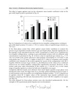
approach for trajectory segmentation.
Fig. 2. Local approach for trajectory segmentation approach overview
2,5
3
3,5
4
4,5
5
5,5
6
6,5
0,9 1,4 1,9 2,4 2,9
Ycoordinate
Xcoordinate
Segmentationissueexample
Trajectoryinputdata Analyzedsegment Analyzedmeasure
Air trafc trajectories segmentation based on time-series sensor data 35
by three sections detailing the three phases for that algorithm when the uniform movement
model is applied: the fourth section will present the different alternatives for the domain
transformation and choose between them the ones included in the final algorithm, the fifth
will present some representative machine learning techniques to be applied to obtain the
classification results and the sixth the filtering refinement over the previous results will be
introduced, leading to the segment synthesis processes. The seventh section will cover the
results obtained over the explained phases, determining the used machine learning
technique and providing the segmentation results, both numerically and graphically, to
provide the reader with easy validation tools over the presented algorithm. Finally a
conclusions section based on the presented results is presented.
2. Problem definition
2.1 General problem definition
As we presented in the introduction section, each analyzed trajectory (
ܶ
) is composed of a
collection of sensor reports (or measurements), which are defined by the following vector:
ݔ
Ԧ
ൌ൫ݔ
ǡݕ
ǡݐ
ǡܴ
൯, ݆߳ሼͳǡǥǡܰ
ሽ
(1)
where j is the measurement number, i the trajectory number, N is the number of
measurements in a given trajectory, ݔ
ǡݕ
are the stereographic projections of the
measurement, ݐ
is the detection time and ܴ
is the covariance matrix (representing the error
introduced by the measuring device). From this problem definition our objective is to divide
our trajectory into a series of segments (
ܤ
ሻ, according to our estimated MOF. This is
performed as an off-line processing (meaning that we may use past and future information
from our trajectory). The segmentation problem can be formalized using the following
notation:
ܶ
ൌ
ڂ
ܤ
ܤ
ൌሼݔ
ሽ ݆߳ሼ݇
ǡǥǡ݇
௫
ሽ
(2)
In the general definition of this problem these segments are obtained by the comparison
with a test model applied over different windows (aggregations) of measurements coming
from our trajectory, in order to obtain a fitness value, deciding finally the segmentation
operation as a function of that fitness value (Mann et al. 2002), (Garcia et al., 2006).
We may consider the division of offline segmentation algorithms into different approaches:
a possible approach is to consider the whole data from the trajectory and the segments
obtained as the problem’s basic division unit (using a global approach), where the basic
operation of the segmentation algorithm is the division of the trajectory into those segments
(examples of this approach are the bottom-up and top-down families (Keogh et al., 2003)). In
the ATC domain, there have been approaches based on a direct adaptation of online
techniques, basically combining the results of forward application of the algorithm (the pure
online technique) with its backward application (applying the online technique reversely to
the time series according to the measurements detection time) (Garcia et al., 2006). An
alternative can be based on the consideration of obtaining a different classification value for
each of the trajectory’s measurements (along with their local information) and obtaining the
segments as a synthesized solution, built upon that classification (basically, by joining those
adjacent measures sharing the same MM into a common segment). This approach allows the
application of several refinements over the classification results before the final synthesis is
performed, and thus is the one explored in the presented solution in this chapter.
2.2 Local approach problem definition
We have presented our problem as an offline processing, meaning that we may use
information both from our past and our future. Introducing this fact into our local
representation, we will restrict that information to a certain local segment around the
measurement which we would like to classify. These intervals are centered on that
measurement, but the boundaries for them can be expressed either in number of
measurements, (3), or according to their detection time values (4).
ܤሺݔ
ሻൌሼݔ
ሽ ݆߳ሾ݉െǡǥǡ݉ǡǥǡ݉ሿ
(3)
ܤሺݔ
ሻൌሼݔ
ሽ ݐ
୨
߳൛ݐ
୫
െǡǥǡ
୫
ǡǥǡݐ
୫
ൟ
(4)
Once we have chosen a window around our current measurement, we will have to apply a
function to that segment in order to obtain its transformed value. This general classification
function F(ݔ
ఫ
ప
ሬ
ሬ
ሬ
Ԧ
ሻ, using measurement boundaries, may be represented with the following
formulation:
F(ݔ
୫
ప
ሬ
ሬ
ሬ
ሬ
ሬ
Ԧ
ሻ = F(ݔ
୫
ప
ሬ
ሬ
ሬ
ሬ
ሬ
Ԧ
ȁܶ
) ֜ F(ݔ
ప
ሬ
ሬ
ሬ
Ԧ
ȁ൫
୫
୧
൯ሻ = F
p
(ݔ
Ԧ
୫ି
, , ݔ
Ԧ
୫
, , ݔ
Ԧ
୫ା
)
(5)
From this formulation of the problem we can already see some of the choices available: how
to choose the segments (according to (3) or (4)), which classification function to apply in (5)
and how to perform the final segment synthesis. Figure 2 shows an example of the local
approach for trajectory segmentation.
Fig. 2. Local approach for trajectory segmentation approach overview
2,5
3
3,5
4
4,5
5
5,5
6
6,5
0,9 1,4 1,9 2,4 2,9
Ycoordinate
Xcoordinate
Segmentationissueexample
Trajectoryinputdata Analyzedsegment Analyzedmeasure
Sensor Fusion and Its Applications36
3. General algorithm proposal
As presented in the introduction section, we will consider three basic MM’s and classify our
measurements individually according to them (Guerrero & Garcia, 2008). If a measurement
is classified as unknown, it will be included in the input data for the next model’s analysis.
This general algorithm introduces a design criterion based on the introduced concepts of
TPR and FPR, respectively equivalent to the type I and type II errors (Allchin, 2001). The
design criterion will be to keep a FPR as low as possible, understanding that those
measurements already assigned to a wrong model will not be analyzed by the following
ones (and thus will remain wrongly classified, leading to a poorer trajectory reconstruction).
The proposed order for this analysis of the MM’s is the same in which they have been
introduced, and the choice is based on how accurately we can represent each of them.
In the local approach problem definition section, the segmentation problem was divided
into two different sub-problems: the definition of the ܨ
ሺݔ
ప
ሬ
ሬ
ሬ
ሬ
ሬ
Ԧ
ሻ function (to perform
measurement classification) and a final segment synthesis over that classification.
According to the different phases presented in the introduction section, we will divide the
definition of the classification function F(ݔ
ఫ
ప
ሬ
ሬ
ሬ
Ԧ
ሻinto two different tasks: a domain
transformation Dtሺݔ
ఫ
ప
ሬ
ሬ
ሬ
Ԧ
ሻ (domain specific, which defines the first phase of our algorithm) and
a final classification Cl(Dtሺݔ
ఫ
ప
ሬ
ሬ
ሬ
Ԧ
ሻ) (based on general classification algorithms, represented by
the data mining techniques which are introduced in the second phase). The final synthesis
over the classification results includes the refinement over that classification introduced by
the filtering process and the actual construction of the output segment (third phase of the
proposed algorithm).
The introduction of the domain transformation Dtሺݔ
ఫ
ప
ሬ
ሬ
ሬ
Ԧ
ሻ from the initial data in the common
reference frame must deal with the following issues: segmentation, (which will cover the
decision of using an independent classification for each measurement or to treat segments as
an indivisible unit), definition for the boundaries of the segments, which involves segment
extension (which analyzes the definition of the segments by number of points or according
to their detection time values) and segment resolution (dealing with the choice of the length
of those segments, and how it affects our results), domain transformations (the different
possible models used in order to obtain an accurate classification in the following phases),
and threshold choosing technique (obtaining a value for a threshold in order to pre-classify
the measurements in the transformed domain).
The second phase introduces a set of machine learning techniques to try to determine
whether each of the measurements belongs to the analyzed model or not, based on the pre-
classifications obtained in the first phase. In this second phase we will have to choose a
Cl(Dtሺݔ
ఫ
ప
ሬ
ሬ
ሬ
Ԧ
ሻ) technique, along with its configuration parameters, to be included in the
algorithm proposal. The considered techniques are decision trees (C4.5, (Quinlan, 1993))
clustering (EM, (Dellaert, 2002)) neural networks (multilayer perceptron, (Gurney, 1997))
and Bayesian nets (Jensen & Graven-Nielsen, 2007) (along with the simplified naive Bayes
approach (Rish, 2001)).
Finally, the third phase (segment synthesis) will propose a filter, based on domain
knowledge, to reanalyze the trajectory classification results and correct those values which
may not follow this knowledge (essentially, based on the required smoothness in MM’s
changes). To obtain the final output for the model analysis, the isolated measurements will
be joined according to their classification in the final segments of the algorithm.
The formalization of these phases and the subsequent changes performed to the data is
presented in the following vectors, representing the input and output data for our three
processes:
Input data:
Domain transformation: Dt
F(
) F(
= {
},
= pre-classification k for measurement j, M = number of pre-classifications included
Classification process: Cl(Dt
)) = Cl({
})=
= automatic classification result for measurement j (including filtering refinement)
Final output:
= Final segments obtained by the union process
4. Domain transformation
The first phase of our algorithm covers the process where we must synthesize an attribute
from our input data to represent each of the trajectory’s measurements in a transformed
domain and choose the appropriate thresholds in that domain to effectively differentiate
those which belong to our model from those which do not do so.
The following aspects are the key parameters for this phase, presented along with the
different alternatives compared for them, (it must be noted that the possibilities compared
here are not the only possible ones, but representative examples of different possible
approaches):
Transformation function: correlation coefficient / Best linear unbiased estimator
residue
Segmentation granularity: segment study / independent study
Segment extension, time / samples, and segment resolution, length of the segment,
using the boundary units imposed by the previous decision
Threshold choosing technique, choice of a threshold to classify data in the
transformed domain.
Each of these parameters requires an individual validation in order to build the actual final
algorithm tested in the experimental section. Each of them will be analyzed in an individual
section in order to achieve this task.
4.1 Transformation function analysis
The transformation function decision is probably the most crucial one involving this first
phase of our algorithm. The comparison presented tries to determine whether there is a real
accuracy increase by introducing noise information (in the form of covariance matrixes).
This section compares a correlation coefficient (Meyer, 1970) (a general statistic with no
noise information) with a BLUE residue (Kay, 1993) (which introduces the noise in the
measuring process). This analysis was originally proposed in (Guerrero & Garcia, 2008). The
equations for the CC statistical are the following:
Air trafc trajectories segmentation based on time-series sensor data 37
3. General algorithm proposal
As presented in the introduction section, we will consider three basic MM’s and classify our
measurements individually according to them (Guerrero & Garcia, 2008). If a measurement
is classified as unknown, it will be included in the input data for the next model’s analysis.
This general algorithm introduces a design criterion based on the introduced concepts of
TPR and FPR, respectively equivalent to the type I and type II errors (Allchin, 2001). The
design criterion will be to keep a FPR as low as possible, understanding that those
measurements already assigned to a wrong model will not be analyzed by the following
ones (and thus will remain wrongly classified, leading to a poorer trajectory reconstruction).
The proposed order for this analysis of the MM’s is the same in which they have been
introduced, and the choice is based on how accurately we can represent each of them.
In the local approach problem definition section, the segmentation problem was divided
into two different sub-problems: the definition of the ܨ
ሺݔ
ప
ሬ
ሬ
ሬ
ሬ
ሬ
Ԧ
ሻ function (to perform
measurement classification) and a final segment synthesis over that classification.
According to the different phases presented in the introduction section, we will divide the
definition of the classification function F(ݔ
ఫ
ప
ሬ
ሬ
ሬ
Ԧ
ሻinto two different tasks: a domain
transformation Dtሺݔ
ఫ
ప
ሬ
ሬ
ሬ
Ԧ
ሻ (domain specific, which defines the first phase of our algorithm) and
a final classification Cl(Dtሺݔ
ఫ
ప
ሬ
ሬ
ሬ
Ԧ
ሻ) (based on general classification algorithms, represented by
the data mining techniques which are introduced in the second phase). The final synthesis
over the classification results includes the refinement over that classification introduced by
the filtering process and the actual construction of the output segment (third phase of the
proposed algorithm).
The introduction of the domain transformation Dtሺݔ
ఫ
ప
ሬ
ሬ
ሬ
Ԧ
ሻ from the initial data in the common
reference frame must deal with the following issues: segmentation, (which will cover the
decision of using an independent classification for each measurement or to treat segments as
an indivisible unit), definition for the boundaries of the segments, which involves segment
extension (which analyzes the definition of the segments by number of points or according
to their detection time values) and segment resolution (dealing with the choice of the length
of those segments, and how it affects our results), domain transformations (the different
possible models used in order to obtain an accurate classification in the following phases),
and threshold choosing technique (obtaining a value for a threshold in order to pre-classify
the measurements in the transformed domain).
The second phase introduces a set of machine learning techniques to try to determine
whether each of the measurements belongs to the analyzed model or not, based on the pre-
classifications obtained in the first phase. In this second phase we will have to choose a
Cl(Dtሺݔ
ఫ
ప
ሬ
ሬ
ሬ
Ԧ
ሻ) technique, along with its configuration parameters, to be included in the
algorithm proposal. The considered techniques are decision trees (C4.5, (Quinlan, 1993))
clustering (EM, (Dellaert, 2002)) neural networks (multilayer perceptron, (Gurney, 1997))
and Bayesian nets (Jensen & Graven-Nielsen, 2007) (along with the simplified naive Bayes
approach (Rish, 2001)).
Finally, the third phase (segment synthesis) will propose a filter, based on domain
knowledge, to reanalyze the trajectory classification results and correct those values which
may not follow this knowledge (essentially, based on the required smoothness in MM’s
changes). To obtain the final output for the model analysis, the isolated measurements will
be joined according to their classification in the final segments of the algorithm.
The formalization of these phases and the subsequent changes performed to the data is
presented in the following vectors, representing the input and output data for our three
processes:
Input data:
Domain transformation: Dt
F(
) F(
= {
},
= pre-classification k for measurement j, M = number of pre-classifications included
Classification process: Cl(Dt
)) = Cl({
})=
= automatic classification result for measurement j (including filtering refinement)
Final output:
= Final segments obtained by the union process
4. Domain transformation
The first phase of our algorithm covers the process where we must synthesize an attribute
from our input data to represent each of the trajectory’s measurements in a transformed
domain and choose the appropriate thresholds in that domain to effectively differentiate
those which belong to our model from those which do not do so.
The following aspects are the key parameters for this phase, presented along with the
different alternatives compared for them, (it must be noted that the possibilities compared
here are not the only possible ones, but representative examples of different possible
approaches):
Transformation function: correlation coefficient / Best linear unbiased estimator
residue
Segmentation granularity: segment study / independent study
Segment extension, time / samples, and segment resolution, length of the segment,
using the boundary units imposed by the previous decision
Threshold choosing technique, choice of a threshold to classify data in the
transformed domain.
Each of these parameters requires an individual validation in order to build the actual final
algorithm tested in the experimental section. Each of them will be analyzed in an individual
section in order to achieve this task.
4.1 Transformation function analysis
The transformation function decision is probably the most crucial one involving this first
phase of our algorithm. The comparison presented tries to determine whether there is a real
accuracy increase by introducing noise information (in the form of covariance matrixes).
This section compares a correlation coefficient (Meyer, 1970) (a general statistic with no
noise information) with a BLUE residue (Kay, 1993) (which introduces the noise in the
measuring process). This analysis was originally proposed in (Guerrero & Garcia, 2008). The
equations for the CC statistical are the following:
Sensor Fusion and Its Applications38
(6)
In order to use the BLUE residue we need to present a model for the uniform MM,
represented in the following equations:
(7)
(8)
With those values we may calculate the interpolated positions for our two variables and the
associated residue:
(9)
(10)
The BLUE residue is presented normalized (the residue divided by the length of the
segment in number of measurements), in order to be able to take advantage of its interesting
statistical properties, which may be used into the algorithm design, and hence allow us to
obtain more accurate results if it is used as our transformation function.
To obtain a classification value from either the CC or the BLUE residue value these values
must be compared with a certain threshold. The CC threshold must be a value close, in
absolute value, to 1, since that indicates a strong correlation between the variables. The
BLUE residue threshold must consider the approximation to a chi-squared function which
can be performed over its value (detailed in the threshold choosing technique section). In
any case, to compare their results and choose the best technique between them, the
threshold can be chosen by means of their TPR and FPR values (choosing manually a
threshold which has zero FPR value with the highest possible TPR value).
To facilitate the performance comparison between the two introduced domain
transformations, we may resort to ROC curves (Fawcett, 2006), which allow us to compare
their behavior by representing their TPR against their FPR. The result of this comparison is
shown in figure 3.
Fig. 3. Comparison between the two presented domain transformations: CC and BLUE
residue
The comparison result shows that the introduction of the sensor’s noise information is vital
for the accuracy of the domain transformation, and thus the BLUE residue is chosen for this
task.
4.2 Segmentation granularity analysis
Having chosen the BLUE residue as the domain transformation function, we intend to
compare the results obtained with two different approaches, regarding the granularity they
apply: the first approach will divide the trajectory into a series of segments of a given size
(which may be expressed, as has been presented, in number of measurements of with
detection time boundaries), obtain their synthesized value and apply that same value to
every measurement belonging to the given segment. On the other hand, we will use the
approach presented in the local definition of the problem, that, for every measurement
belonging to the trajectory, involves choosing a segment around the given measurement,
obtain its surrounding segment and find its transformed value according to that segment
(which is applied only to the central measurement of the segment, not to every point
belonging to it).
There are a number of considerations regarding this comparison: obviously, the results
achieved by the local approach obtaining a different transformed value for each
measurement will be more precise than those obtained by its alternative, but it will also
involve a greater computational complexity. Considering a segment size of s_size and a
trajectory with n measurements, the complexity of obtaining a transformed value for each of
these measurements is Ȫሺ݊כݏ̴ݏ݅ݖ݁ሻ whereas obtaining only a value and applying it to the
whole segment is Ȫሺ݊ሻ, introducing efficiency factors which we will ignore due to the offline
nature of the algorithm.
Another related issue is the restrictions which applying the same transformed value to the
whole segment introduces regarding the choice of those segments boundaries. If the
transformed value is applied only to the central measurement, we may choose longer of
Air trafc trajectories segmentation based on time-series sensor data 39
(6)
In order to use the BLUE residue we need to present a model for the uniform MM,
represented in the following equations:
(7)
(8)
With those values we may calculate the interpolated positions for our two variables and the
associated residue:
(9)
(10)
The BLUE residue is presented normalized (the residue divided by the length of the
segment in number of measurements), in order to be able to take advantage of its interesting
statistical properties, which may be used into the algorithm design, and hence allow us to
obtain more accurate results if it is used as our transformation function.
To obtain a classification value from either the CC or the BLUE residue value these values
must be compared with a certain threshold. The CC threshold must be a value close, in
absolute value, to 1, since that indicates a strong correlation between the variables. The
BLUE residue threshold must consider the approximation to a chi-squared function which
can be performed over its value (detailed in the threshold choosing technique section). In
any case, to compare their results and choose the best technique between them, the
threshold can be chosen by means of their TPR and FPR values (choosing manually a
threshold which has zero FPR value with the highest possible TPR value).
To facilitate the performance comparison between the two introduced domain
transformations, we may resort to ROC curves (Fawcett, 2006), which allow us to compare
their behavior by representing their TPR against their FPR. The result of this comparison is
shown in figure 3.
Fig. 3. Comparison between the two presented domain transformations: CC and BLUE
residue
The comparison result shows that the introduction of the sensor’s noise information is vital
for the accuracy of the domain transformation, and thus the BLUE residue is chosen for this
task.
4.2 Segmentation granularity analysis
Having chosen the BLUE residue as the domain transformation function, we intend to
compare the results obtained with two different approaches, regarding the granularity they
apply: the first approach will divide the trajectory into a series of segments of a given size
(which may be expressed, as has been presented, in number of measurements of with
detection time boundaries), obtain their synthesized value and apply that same value to
every measurement belonging to the given segment. On the other hand, we will use the
approach presented in the local definition of the problem, that, for every measurement
belonging to the trajectory, involves choosing a segment around the given measurement,
obtain its surrounding segment and find its transformed value according to that segment
(which is applied only to the central measurement of the segment, not to every point
belonging to it).
There are a number of considerations regarding this comparison: obviously, the results
achieved by the local approach obtaining a different transformed value for each
measurement will be more precise than those obtained by its alternative, but it will also
involve a greater computational complexity. Considering a segment size of s_size and a
trajectory with n measurements, the complexity of obtaining a transformed value for each of
these measurements is Ȫሺ݊כݏ̴ݏ݅ݖ݁ሻ whereas obtaining only a value and applying it to the
whole segment is Ȫሺ݊ሻ, introducing efficiency factors which we will ignore due to the offline
nature of the algorithm.
Another related issue is the restrictions which applying the same transformed value to the
whole segment introduces regarding the choice of those segments boundaries. If the
transformed value is applied only to the central measurement, we may choose longer of
Sensor Fusion and Its Applications40
shorter segments according to the transformation results (this choice will be analysed in the
following section), while applying that same transformed value to the whole segments
introduces restrictions related to the precision which that length introduces (longer
segments may be better to deal with the noise in the measurements, but, at the same time,
obtain worse results due to applying the same transformed value to a greater number of
measurements).
The ROC curve results for this comparison, using segments composed of thirty-one
measurements, are shown in figure 4.
Fig. 4. Comparison between the two presented granularity choices
Given the presented design criterion, which remarks the importance of low FPR values, we
may see that individual transformed values perform much better at that range (leftmost side
of the figure), leading us, along with the considerations previously exposed, to its choice for
the algorithm final implementation.
4.3 Segment definition analysis
The definition of the segments we will analyze involves two different factors: the boundary
units used and the length (and its effects on the results) of those segments (respectively
referred to as segment extension and segment resolution in this phase’s presentation). One
of the advantages of building domain-dependent algorithms is the use of information
belonging to that domain. In the particular case of the ATC domain, we will have
information regarding the lengths of the different possible manoeuvres performed by the
aircrafts, and will base our segments in those lengths. This information will usually come in
the form of time intervals (for example, the maximum and minimum duration of turn
manoeuvres in seconds), but may also come in the form on number of detections in a given
zone of interest. Thus, the choice of one or the other (respectively represented in the
problem definition section by equations (4) and (3)) will be based on the available
information.
With the units given by the available information, Figure 5 shows the effect of different
resolutions over a given turn trajectory, along with the results over those resolutions.
Fig. 5. Comparison of transformed domain values and pre-classification results
Air trafc trajectories segmentation based on time-series sensor data 41
shorter segments according to the transformation results (this choice will be analysed in the
following section), while applying that same transformed value to the whole segments
introduces restrictions related to the precision which that length introduces (longer
segments may be better to deal with the noise in the measurements, but, at the same time,
obtain worse results due to applying the same transformed value to a greater number of
measurements).
The ROC curve results for this comparison, using segments composed of thirty-one
measurements, are shown in figure 4.
Fig. 4. Comparison between the two presented granularity choices
Given the presented design criterion, which remarks the importance of low FPR values, we
may see that individual transformed values perform much better at that range (leftmost side
of the figure), leading us, along with the considerations previously exposed, to its choice for
the algorithm final implementation.
4.3 Segment definition analysis
The definition of the segments we will analyze involves two different factors: the boundary
units used and the length (and its effects on the results) of those segments (respectively
referred to as segment extension and segment resolution in this phase’s presentation). One
of the advantages of building domain-dependent algorithms is the use of information
belonging to that domain. In the particular case of the ATC domain, we will have
information regarding the lengths of the different possible manoeuvres performed by the
aircrafts, and will base our segments in those lengths. This information will usually come in
the form of time intervals (for example, the maximum and minimum duration of turn
manoeuvres in seconds), but may also come in the form on number of detections in a given
zone of interest. Thus, the choice of one or the other (respectively represented in the
problem definition section by equations (4) and (3)) will be based on the available
information.
With the units given by the available information, Figure 5 shows the effect of different
resolutions over a given turn trajectory, along with the results over those resolutions.
Fig. 5. Comparison of transformed domain values and pre-classification results
Sensor Fusion and Its Applications42
Observing the presented results, where the threshold has been calculated according to the
procedure explained in the following section, we may determine the resolution effects: short
segments exhibit several handicaps: on the one hand, they are more susceptible to the noise
effects, and, on the other hand, in some cases, long smooth non-uniform MM segments may
be accurately approximated with short uniform segments, causing the algorithm to bypass
them (these effects can be seen in the lower resolutions shown in figure 5). Longer segments
allow us to treat the noise effects more effectively (with resolution 31 there are already no
misclassified measurements during non-uniform segments) and make the identification of
non-uniform segments possible, avoiding the possibility of obtaining an accurate
approximation of these segments using uniform ones (as can be seen with resolution 91)
However, long segments also make the measurements close to a non-uniform MM increase
their transformed value (as their surrounding segment starts to get into the non-uniform
MM), leading to the fact that more measurements around the non-uniform segments will be
pre-classified incorrectly as non-uniform (resolution 181). A different example of the effects
of resolution in these pre-classification results may be looked up in (Guerrero et al., 2010).
There is, as we have seen, no clear choice for a single resolution value. Lower resolutions
may allow us to obtain more precise results at the beginning and end of non-uniform
segments, while higher resolution values are capital to guarantee the detection of those non-
uniform segments and the appropriate treatment of the measurements noise. Thus, for this
first phase, a multi-resolution approach will be used, feeding the second phase with the
different pre-classifications of the algorithm according to different resolution values.
4.4 Threshold choosing technique
The threshold choice involves automatically determining the boundary above which
transformed measurements will be considered as unknown. Examples of this choice may be
seen in the previous section (figure 5). According to our design criterion, we would like to
obtain a TPR as high as possible keeping our FPR ideally at a zero value. Graphically over
the examples in figure 5 (especially for the highest resolutions, where the non-uniform
maneuver can be clearly identified), that implies getting the red line as low as possible,
leaving only the central section over it (where the maneuver takes place, making its residue
value high enough to get over our threshold).
As presented in (Guerrero et al., 2010), the residue value in (10) follows a Chi-squared
probability distribution function (pdf) normalized by its degrees of freedom, n. The value of
n is given by twice the number of 2D measurements contained in the interval minus the
dimension of P (P=4 in the presented uniform model, as we are imposing 4 linear
restrictions). For a valid segment residual, “res” behaves with distribution
ଵ
ሺ
௫ିାଵ
ሻ
߯
ଶ
ሺ
௫ିାଵ
ሻ
ି
ଶ
, which has the following mean and variance:
ߤൌʹെ
ሺ
௫ିାଵ
ሻ
ߪ
ଶ
ൌ
ସ
ሺ
௫ିାଵ
ሻ
െ
ଶ
ሺ
௫ିାଵ
ሻ
మ
(11)
The residue distribution allows us to establish our criterion based on the TPR value, but not
the FPR (we have a distribution over the uniform measurements, not the unknown ones),
which is the one constrained by the design criterion. We may use the Chevychev’s
inequality (Meyer, 1970) to determine a threshold which should leave the 99% of the
measurements belonging to our model above it (TPR>=0.99), with ߤ͵ߪ value. From the
values exposed in (11) we get the following threshold value:
thres=ʹെ
ସ
ே
͵
ට
ସ
ே
െ
଼
ே
మ
ܰൌ
ሺ
݇݉ܽݔെ݇݉݅݊ͳ
ሻ
(12)
This threshold depends on the resolution of the segment, N, which also influences the
residue value in (10). It is interesting to notice that the highest threshold value is reached
with the lowest resolution. This is a logical result, since to be able to maintain the TPR value
(having fixed it with the inequality at 99%) with short segments, a high threshold value is
required, in order to counteract the noise effects (while longer segments are more resistant
to that noise and thus the threshold value may be lower).
We would like to determine how precisely our ߯
ଶ
distribution represents our normalized
residue in non-uniform trajectories with estimated covariance matrix. In the following
figures we compare the optimal result of the threshold choice (dotted lines), manually
chosen, to the results obtained with equation (12). Figure 6 shows the used trajectories for
this comparison, along with the proposed comparison between the optimal TPR and the one
obtained with (12) for increasing threshold values.
Fig. 6. Comparison of transformed domain values and pre-classification results
In the two trajectories in figure 6 we may appreciate two different distortion effects
introduced by our approximation. The turn trajectory shows an underestimation of our TPR
due to the inexactitude in the covariance matrix ܴ
. This inexactitude assumes a higher
noise than the one which is present in the trajectory, and thus will make us choose a higher
threshold than necessary in order to obtain the desired TPR margin.
In the racetrack trajectory we perceive the same underestimation at the lower values of the
threshold, but then our approximation crosses the optimal results and reaches a value over
it. This is caused by the second distortion effect, the maneuver’s edge measurements. The
measurements close to a maneuver beginning or end tend to have a higher residue value
Air trafc trajectories segmentation based on time-series sensor data 43
Observing the presented results, where the threshold has been calculated according to the
procedure explained in the following section, we may determine the resolution effects: short
segments exhibit several handicaps: on the one hand, they are more susceptible to the noise
effects, and, on the other hand, in some cases, long smooth non-uniform MM segments may
be accurately approximated with short uniform segments, causing the algorithm to bypass
them (these effects can be seen in the lower resolutions shown in figure 5). Longer segments
allow us to treat the noise effects more effectively (with resolution 31 there are already no
misclassified measurements during non-uniform segments) and make the identification of
non-uniform segments possible, avoiding the possibility of obtaining an accurate
approximation of these segments using uniform ones (as can be seen with resolution 91)
However, long segments also make the measurements close to a non-uniform MM increase
their transformed value (as their surrounding segment starts to get into the non-uniform
MM), leading to the fact that more measurements around the non-uniform segments will be
pre-classified incorrectly as non-uniform (resolution 181). A different example of the effects
of resolution in these pre-classification results may be looked up in (Guerrero et al., 2010).
There is, as we have seen, no clear choice for a single resolution value. Lower resolutions
may allow us to obtain more precise results at the beginning and end of non-uniform
segments, while higher resolution values are capital to guarantee the detection of those non-
uniform segments and the appropriate treatment of the measurements noise. Thus, for this
first phase, a multi-resolution approach will be used, feeding the second phase with the
different pre-classifications of the algorithm according to different resolution values.
4.4 Threshold choosing technique
The threshold choice involves automatically determining the boundary above which
transformed measurements will be considered as unknown. Examples of this choice may be
seen in the previous section (figure 5). According to our design criterion, we would like to
obtain a TPR as high as possible keeping our FPR ideally at a zero value. Graphically over
the examples in figure 5 (especially for the highest resolutions, where the non-uniform
maneuver can be clearly identified), that implies getting the red line as low as possible,
leaving only the central section over it (where the maneuver takes place, making its residue
value high enough to get over our threshold).
As presented in (Guerrero et al., 2010), the residue value in (10) follows a Chi-squared
probability distribution function (pdf) normalized by its degrees of freedom, n. The value of
n is given by twice the number of 2D measurements contained in the interval minus the
dimension of P (P=4 in the presented uniform model, as we are imposing 4 linear
restrictions). For a valid segment residual, “res” behaves with distribution
ଵ
ሺ
௫ିାଵ
ሻ
߯
ଶ
ሺ
௫ିାଵ
ሻ
ି
ଶ
, which has the following mean and variance:
ߤൌʹെ
ሺ
௫ିାଵ
ሻ
ߪ
ଶ
ൌ
ସ
ሺ
௫ିାଵ
ሻ
െ
ଶ
ሺ
௫ିାଵ
ሻ
మ
(11)
The residue distribution allows us to establish our criterion based on the TPR value, but not
the FPR (we have a distribution over the uniform measurements, not the unknown ones),
which is the one constrained by the design criterion. We may use the Chevychev’s
inequality (Meyer, 1970) to determine a threshold which should leave the 99% of the
measurements belonging to our model above it (TPR>=0.99), with ߤ͵ߪ value. From the
values exposed in (11) we get the following threshold value:
thres=ʹെ
ସ
ே
͵
ට
ସ
ே
െ
଼
ே
మ
ܰൌ
ሺ
݇݉ܽݔെ݇݉݅݊ͳ
ሻ
(12)
This threshold depends on the resolution of the segment, N, which also influences the
residue value in (10). It is interesting to notice that the highest threshold value is reached
with the lowest resolution. This is a logical result, since to be able to maintain the TPR value
(having fixed it with the inequality at 99%) with short segments, a high threshold value is
required, in order to counteract the noise effects (while longer segments are more resistant
to that noise and thus the threshold value may be lower).
We would like to determine how precisely our ߯
ଶ
distribution represents our normalized
residue in non-uniform trajectories with estimated covariance matrix. In the following
figures we compare the optimal result of the threshold choice (dotted lines), manually
chosen, to the results obtained with equation (12). Figure 6 shows the used trajectories for
this comparison, along with the proposed comparison between the optimal TPR and the one
obtained with (12) for increasing threshold values.
Fig. 6. Comparison of transformed domain values and pre-classification results
In the two trajectories in figure 6 we may appreciate two different distortion effects
introduced by our approximation. The turn trajectory shows an underestimation of our TPR
due to the inexactitude in the covariance matrix ܴ
. This inexactitude assumes a higher
noise than the one which is present in the trajectory, and thus will make us choose a higher
threshold than necessary in order to obtain the desired TPR margin.
In the racetrack trajectory we perceive the same underestimation at the lower values of the
threshold, but then our approximation crosses the optimal results and reaches a value over
it. This is caused by the second distortion effect, the maneuver’s edge measurements. The
measurements close to a maneuver beginning or end tend to have a higher residue value
Sensor Fusion and Its Applications44
than the theoretical one for a uniform trajectory (due to their proximity to the non-uniform
segments), making us increase the threshold value to classify them correctly (which causes
the optimal result to show a lower TPR in the figure). These two effects show that a heuristic
tuning may be required in our ߯
ଶ
distribution in order to adapt it to these distortion effects.
5. Machine learning techniques application
The algorithm’s first phase, as has been detailed, ended with a set of pre-classification
values based on the application of the domain transformation with different resolutions to
every measurement in the trajectory. The objective of this second phase is to obtain a
classification according to the analyzed model for each of these measurements, to be able to
build the resulting segments from this data.
There are countless variants of machine learning techniques, so the choice of the ones
presented here was not a trivial one. There was not a particular family of them more
promising a-priori, so the decision tried to cover several objectives: they should be easy to
replicate, general and, at the same time, cover different approaches in order to give the
algorithm the chance to include the best alternative from a wide set of choices. This led to
the choice of Weka®
1
as the integrated tool for these tests, trying to use the algorithms with
their default parameters whenever possible (it will be indicated otherwise if necessary),
even though the fine tuning of them gives us a very slight better performance, and the
choice of representative well tested algorithms from different important families in machine
learning: decision trees (C4.5) clustering (EM) neural networks (multilayer perceptron) and
Bayesian networks, along with the simplified naive Bayes approach. We will describe each
of these techniques briefly.
Decision trees are predictive models based on a set of “attribute-value” pairs and the
entropy heuristic. The C 4.5 algorithm (Quinlan, 1993) allows continuous values for its
variables.
Clustering techniques have the objective of grouping together examples with similar
characteristics and obtain a series of models for them that, even though they may not cover
all the characteristics of their represented members, can be representative enough of their
sets as a whole (this definition adapts very well to the case in this chapter, since we want to
obtain a representative set of common characteristics for measurements following our
analyzed model). The EM algorithm (Dellaert, 2002) is based on a statistical model which
represents the input data basing itself on the existence of k Gaussian probability distribution
functions, each of them representing a different cluster. These functions are based on
maximum likelihood hypothesis. It is important to realize that this is an unsupervised
technique which does not classify our data, only groups it. In our problem, we will have to
select the classification label afterwards for each cluster. In this algorithm, as well, we will
introduce a non standard parameter for the number of clusters. The default configuration
allows Weka to automatically determine this number, but, in our case, we only want two
different clusters: one representing those measurements following the analyzed model and a
different one for those unknown, so we will introduce this fact in the algorithm’s
configuration.
1
Available online at
Bayesian networks (Jensen & Graven-Nielsen, 2007) are directed acyclic graphs whose nodes
represent variables, and whose missing edges encode conditional independencies between
the variables. Nodes can represent any kind of variable, be it a measured parameter, a latent
variable or a hypothesis. Special simplifications of these networks are Naive Bayes networks
(Rish, 2001), where the variables are considered independent. This supposition, even though
it may be considered a very strong one, usually introduces a faster learning when the
number of training samples is low, and in practice achieves very good results.
Artificial neural networks are computational models based on biological neural networks,
consisting of an interconnected group of artificial neurons, which process information using
a connectionist approach to computation. Multilayer Perceptron (MP), (Gurney, 1997), are
feed-forward neural networks having an input layer, an undetermined number of hidden
layers and an output layer, with nonlinear activation functions. MP’s are universal function
approximators, and thus they are able to distinguish non-linearly separable data. One of the
handicaps of their approach is the configuration difficulties which they exhibit (dealing
mainly with the number of neurons and hidden layers required for the given problem). The
Weka tool is able to determine these values automatically.
6. Classification refinement and segment construction
The algorithm’s final phase must refine the results from the machine learning techniques
and build the appropriate segments from the individual measurements classification. To
perform this refinement, we will use the continuity in the movement of the aircrafts,
meaning that no abrupt MM changes can be performed (every MM has to be sustained for a
certain time-length). This means that situations where a certain measurement shows a
classification value different to its surrounding values can be corrected assigning to it the
one shared by its neighbours.
This correction will be performed systematically by means of a voting system, assigning the
most repeated classification in its segment to the central measurement. This processing is
similar to the one performed by median filters (Yin et al., 1996) widely used in image
processing (Baxes, 1994).
The widow size for this voting system has to be determined. In the segment definition
section the importance of the available information regarding the length of the possible non-
uniform MM’s was pointed out, in order to determine the resolution of the domain
transformation, which is used as well for this window size definition. Choosing a too high
value for our window size might cause the algorithm to incorrectly reclassify non-uniform
measurements as uniform (if its value exceeds the length of the non-uniform segment they
belong to) leading to an important increase in the FPR value (while the design criterion tries
to avoid this fact during the three phases presented). Thus, the window size will have the
value of the shortest possible non-uniform MM.
It also important to determine which measurements must be treated with this filtering
process. Through the different previous phases the avoidance of FPR has been highlighted
(by means of multi-resolution domain transformation and the proper election of the used
machine learning technique), even at the cost of slightly decreasing the TPR value. Those
considerations are followed in this final phase by the application of this filtering process
only to measurements classified as non-uniform, due to their possible misclassification
Air trafc trajectories segmentation based on time-series sensor data 45
than the theoretical one for a uniform trajectory (due to their proximity to the non-uniform
segments), making us increase the threshold value to classify them correctly (which causes
the optimal result to show a lower TPR in the figure). These two effects show that a heuristic
tuning may be required in our ߯
ଶ
distribution in order to adapt it to these distortion effects.
5. Machine learning techniques application
The algorithm’s first phase, as has been detailed, ended with a set of pre-classification
values based on the application of the domain transformation with different resolutions to
every measurement in the trajectory. The objective of this second phase is to obtain a
classification according to the analyzed model for each of these measurements, to be able to
build the resulting segments from this data.
There are countless variants of machine learning techniques, so the choice of the ones
presented here was not a trivial one. There was not a particular family of them more
promising a-priori, so the decision tried to cover several objectives: they should be easy to
replicate, general and, at the same time, cover different approaches in order to give the
algorithm the chance to include the best alternative from a wide set of choices. This led to
the choice of Weka®
1
as the integrated tool for these tests, trying to use the algorithms with
their default parameters whenever possible (it will be indicated otherwise if necessary),
even though the fine tuning of them gives us a very slight better performance, and the
choice of representative well tested algorithms from different important families in machine
learning: decision trees (C4.5) clustering (EM) neural networks (multilayer perceptron) and
Bayesian networks, along with the simplified naive Bayes approach. We will describe each
of these techniques briefly.
Decision trees are predictive models based on a set of “attribute-value” pairs and the
entropy heuristic. The C 4.5 algorithm (Quinlan, 1993) allows continuous values for its
variables.
Clustering techniques have the objective of grouping together examples with similar
characteristics and obtain a series of models for them that, even though they may not cover
all the characteristics of their represented members, can be representative enough of their
sets as a whole (this definition adapts very well to the case in this chapter, since we want to
obtain a representative set of common characteristics for measurements following our
analyzed model). The EM algorithm (Dellaert, 2002) is based on a statistical model which
represents the input data basing itself on the existence of k Gaussian probability distribution
functions, each of them representing a different cluster. These functions are based on
maximum likelihood hypothesis. It is important to realize that this is an unsupervised
technique which does not classify our data, only groups it. In our problem, we will have to
select the classification label afterwards for each cluster. In this algorithm, as well, we will
introduce a non standard parameter for the number of clusters. The default configuration
allows Weka to automatically determine this number, but, in our case, we only want two
different clusters: one representing those measurements following the analyzed model and a
different one for those unknown, so we will introduce this fact in the algorithm’s
configuration.
1
Available online at
Bayesian networks (Jensen & Graven-Nielsen, 2007) are directed acyclic graphs whose nodes
represent variables, and whose missing edges encode conditional independencies between
the variables. Nodes can represent any kind of variable, be it a measured parameter, a latent
variable or a hypothesis. Special simplifications of these networks are Naive Bayes networks
(Rish, 2001), where the variables are considered independent. This supposition, even though
it may be considered a very strong one, usually introduces a faster learning when the
number of training samples is low, and in practice achieves very good results.
Artificial neural networks are computational models based on biological neural networks,
consisting of an interconnected group of artificial neurons, which process information using
a connectionist approach to computation. Multilayer Perceptron (MP), (Gurney, 1997), are
feed-forward neural networks having an input layer, an undetermined number of hidden
layers and an output layer, with nonlinear activation functions. MP’s are universal function
approximators, and thus they are able to distinguish non-linearly separable data. One of the
handicaps of their approach is the configuration difficulties which they exhibit (dealing
mainly with the number of neurons and hidden layers required for the given problem). The
Weka tool is able to determine these values automatically.
6. Classification refinement and segment construction
The algorithm’s final phase must refine the results from the machine learning techniques
and build the appropriate segments from the individual measurements classification. To
perform this refinement, we will use the continuity in the movement of the aircrafts,
meaning that no abrupt MM changes can be performed (every MM has to be sustained for a
certain time-length). This means that situations where a certain measurement shows a
classification value different to its surrounding values can be corrected assigning to it the
one shared by its neighbours.
This correction will be performed systematically by means of a voting system, assigning the
most repeated classification in its segment to the central measurement. This processing is
similar to the one performed by median filters (Yin et al., 1996) widely used in image
processing (Baxes, 1994).
The widow size for this voting system has to be determined. In the segment definition
section the importance of the available information regarding the length of the possible non-
uniform MM’s was pointed out, in order to determine the resolution of the domain
transformation, which is used as well for this window size definition. Choosing a too high
value for our window size might cause the algorithm to incorrectly reclassify non-uniform
measurements as uniform (if its value exceeds the length of the non-uniform segment they
belong to) leading to an important increase in the FPR value (while the design criterion tries
to avoid this fact during the three phases presented). Thus, the window size will have the
value of the shortest possible non-uniform MM.
It also important to determine which measurements must be treated with this filtering
process. Through the different previous phases the avoidance of FPR has been highlighted
(by means of multi-resolution domain transformation and the proper election of the used
machine learning technique), even at the cost of slightly decreasing the TPR value. Those
considerations are followed in this final phase by the application of this filtering process
only to measurements classified as non-uniform, due to their possible misclassification
Sensor Fusion and Its Applications46
caused by their surrounding noise. Figure 7 shows the results of this filtering process
applied to an accelerated trajectory
Fig. 7. Example filtering process applied to an accelerated trajectory
In figure 7, the lowest values (0.8 for post-filtered results, 0.9 for pre-filtered ones and 1 for
the real classification) indicate that the measurement is classified as uniform, whereas their
respective higher ones (1+ its lowest value) indicate that the measurement is classified as
non-uniform. This figure shows that some measurements previously misclassified as non-
uniform are corrected.
The importance of this filtering phase is not usually reflected in the TPR, bearing in mind
that the number of measurements affected by it may be very small, but the number of
output segments can vary its value significantly. In the example in figure 7, the pre-filtered
classification would have output nine different segments, whereas the post-filtered
classification outputs only three segments. This change highlights the importance of this
filtering process.
The method to obtain the output segments is extremely simple after this median filter
application: starting from the first detected measurement, one segment is built according to
that measurement classification, until another measurement i with a different classification
value is found. At that point, the first segment is defined with boundaries [1, i-1] and the
process is restarted at measurement i, repeating this cycle until the end of the trajectory is
reached.
7. Experimental validation
The division of the algorithm into different consecutive phases introduces validation
difficulties, as the results are mutually dependant. In this whole work, we have tried to
show those validations along with the techniques explanation when it was unavoidable (as
occurred in the first phase, due to the influence of the choices in its different parameters)
and postpone the rest of the cases for a final validation over a well defined test set (second
and third phases, along with the overall algorithm performance).
This validation process is carried out by the generation of a set of test trajectories as
representative as possible, implying not to use exact covariance matrixes, (but estimations of
their value), and carefully choosing the shapes of the simulated trajectories. We have based
our results on four kind of simulated trajectories, each having two different samples.
Uniform, turn and accelerated trajectories are a direct validation of our three basic MM’s
identified, while the fourth trajectory type, racetrack, is a typical situation during landing
procedures.
This validation will be divided into three different steps: the first one will use the whole
data from these trajectories, obtain the transformed multi-resolution values for each
measurement and apply the different presented machine learning techniques, analyzing the
obtained results and choosing a particular technique to be included in the algorithm as a
consequence of those results.
Having determined the used technique, the second step will apply the described refinement
process to those classifications, obtaining the final classification results (along with their TPR
and FPR values). Finally the segmentations obtained for each trajectory are shown along
with the real classification of each trajectory, to allow the reader to perform a graphical
validation of the final results.
7.1 Machine learning techniques validation
The validation method for the machine learning techniques still has to be determined. The
chosen method is cross-validation (Picard and Cook, 1984) with 10 folds. This method
ensures robustness in the percentages shown. The results output format for any of these
techniques in Weka provides us with the number of correctly and incorrectly classified
measurements, along with the confusion matrix, detailing the different class assignations. In
order to use these values into our algorithm’s framework, they have to be transformed into
TPR and FPR values. They can be obtained from the confusion matrix, as shown in the
following example:
Weka’s raw output:
Correctly Classified Instances 10619 96.03 %
Incorrectly Classified Instances 439 3.97 %
=== Confusion Matrix ===
a b < classified as
345 37 | a = uniform_model
0 270 | b = unknown_model
Algorithm parameters:
TPR = 345/37 = 0,903141361 FPR = 0/270 = 0
The selection criterion from these values must consider the design criterion of keeping a FPR
value as low as possible, trying to obtain, at the same time, the highest possible TPR value.
Also, we have introduced as their input only six transformed values for each measurement,
corresponding to resolutions 11, 31, 51, 71, 91 and 111 (all of them expressed in number of
measurements) The results presentation shown in table 1 provides the individual results for
each trajectory, along with the results when the whole dataset is used as its input. The
individual results do not include the completely uniform trajectories (due to their lack of
FPR, having no non-uniform measurements). Figure 8 shows the graphical comparison of
the different algorithms with the whole dataset according to their TPR and FPR values
Air trafc trajectories segmentation based on time-series sensor data 47
caused by their surrounding noise. Figure 7 shows the results of this filtering process
applied to an accelerated trajectory
Fig. 7. Example filtering process applied to an accelerated trajectory
In figure 7, the lowest values (0.8 for post-filtered results, 0.9 for pre-filtered ones and 1 for
the real classification) indicate that the measurement is classified as uniform, whereas their
respective higher ones (1+ its lowest value) indicate that the measurement is classified as
non-uniform. This figure shows that some measurements previously misclassified as non-
uniform are corrected.
The importance of this filtering phase is not usually reflected in the TPR, bearing in mind
that the number of measurements affected by it may be very small, but the number of
output segments can vary its value significantly. In the example in figure 7, the pre-filtered
classification would have output nine different segments, whereas the post-filtered
classification outputs only three segments. This change highlights the importance of this
filtering process.
The method to obtain the output segments is extremely simple after this median filter
application: starting from the first detected measurement, one segment is built according to
that measurement classification, until another measurement i with a different classification
value is found. At that point, the first segment is defined with boundaries [1, i-1] and the
process is restarted at measurement i, repeating this cycle until the end of the trajectory is
reached.
7. Experimental validation
The division of the algorithm into different consecutive phases introduces validation
difficulties, as the results are mutually dependant. In this whole work, we have tried to
show those validations along with the techniques explanation when it was unavoidable (as
occurred in the first phase, due to the influence of the choices in its different parameters)
and postpone the rest of the cases for a final validation over a well defined test set (second
and third phases, along with the overall algorithm performance).
This validation process is carried out by the generation of a set of test trajectories as
representative as possible, implying not to use exact covariance matrixes, (but estimations of
their value), and carefully choosing the shapes of the simulated trajectories. We have based
our results on four kind of simulated trajectories, each having two different samples.
Uniform, turn and accelerated trajectories are a direct validation of our three basic MM’s
identified, while the fourth trajectory type, racetrack, is a typical situation during landing
procedures.
This validation will be divided into three different steps: the first one will use the whole
data from these trajectories, obtain the transformed multi-resolution values for each
measurement and apply the different presented machine learning techniques, analyzing the
obtained results and choosing a particular technique to be included in the algorithm as a
consequence of those results.
Having determined the used technique, the second step will apply the described refinement
process to those classifications, obtaining the final classification results (along with their TPR
and FPR values). Finally the segmentations obtained for each trajectory are shown along
with the real classification of each trajectory, to allow the reader to perform a graphical
validation of the final results.
7.1 Machine learning techniques validation
The validation method for the machine learning techniques still has to be determined. The
chosen method is cross-validation (Picard and Cook, 1984) with 10 folds. This method
ensures robustness in the percentages shown. The results output format for any of these
techniques in Weka provides us with the number of correctly and incorrectly classified
measurements, along with the confusion matrix, detailing the different class assignations. In
order to use these values into our algorithm’s framework, they have to be transformed into
TPR and FPR values. They can be obtained from the confusion matrix, as shown in the
following example:
Weka’s raw output:
Correctly Classified Instances 10619 96.03 %
Incorrectly Classified Instances 439 3.97 %
=== Confusion Matrix ===
a b < classified as
345 37 | a = uniform_model
0 270 | b = unknown_model
Algorithm parameters:
TPR = 345/37 = 0,903141361 FPR = 0/270 = 0
The selection criterion from these values must consider the design criterion of keeping a FPR
value as low as possible, trying to obtain, at the same time, the highest possible TPR value.
Also, we have introduced as their input only six transformed values for each measurement,
corresponding to resolutions 11, 31, 51, 71, 91 and 111 (all of them expressed in number of
measurements) The results presentation shown in table 1 provides the individual results for
each trajectory, along with the results when the whole dataset is used as its input. The
individual results do not include the completely uniform trajectories (due to their lack of
FPR, having no non-uniform measurements). Figure 8 shows the graphical comparison of
the different algorithms with the whole dataset according to their TPR and FPR values