Sensor Fusion and its Applications Part 13 ppt

Sensor Fusion and Its Applications354

2 2
0 0
d d
and
 
 
 
 
(7)
Line parameters can be determined by the following


2 2
2 2
2 ( )( )
tan(2 )
[( ) ( ) ]
2 ( )( )
0.5 tan 2
[( ) ( ) ]
m i m i
m i m i
m i m i
m i m i
y y x x
y y x x
y y x x
a

y y x x


  

  
 
  

 
 
  
 




(8)

if we assume that the Centroid is on the line then

can be computed using equation 4 as:


cos( ) sin( )
m m
x y

 
  (9)

where

1
1
m i
m i
x
x
N
and
y
y
N




(10)

are (
m
x
,
m
y
) are Cartesian coordinates of the Centroid, and N is the number of points in the
sector scan we wish to fit line parameter to.

Fig. 7. Fitting lines to a laser scan. A line has more than four sample points.

During the line fitting process, further splitting positions within a cluster are determined by
computing perpendicular distance of each point to the fitted line. As shown by figure 6. A
point where the perpendicular distance is greater than the tolerance value is marked as a
candidate splitting position. The process is iteratively done until the whole cluster scan is
made up of linear sections as depicted by figure 7 above. The next procedure is collection of
endpoints, which is joining points of lines closest to each other. This is how corner positions
are determined from split and merge algorithm. The figure below shows extracted corners
defined at positions where two line meet. These positions (corners) are marked in pink.


Fig. 8. Splitting position taken as corners (pink marks) viewed from successive robot
positions. The first and second extraction shows 5 corners. Interestingly, in the second
extraction a corner is noted at a new position, In SLAM, the map has total of 6 landmarks in
the state vector instead of 5. The association algorithm will not associate the corners; hence a
new feature is mapped corrupting the map.

The split and merge corner detector brings up many possible corners locations. This has a
high probability of corrupting the map because some corners are ‘ghosts’. There is also the
issue of computation burden brought about by the number of landmarks in the map. The
standard EKF-SLAM requires time quadratic in the number of features in the map (Thrun, S
et al. 2002).This computational burden restricts EKF-SLAM to medium sized environments
with no more than a few hundred features.

Feature extraction: techniques for landmark based navigation system 355

2 2
0 0
d d

and
 
 


 
(7)
Line parameters can be determined by the following


2 2
2 2
2 ( )( )
tan(2 )
[( ) ( ) ]
2 ( )( )
0.5 tan 2
[( ) ( ) ]
m i m i
m i m i
m i m i
m i m i
y y x x
y y x x
y y x x
a
y y x x


  


  
 
  

 
 
  
 




(8)

if we assume that the Centroid is on the line then

can be computed using equation 4 as:


cos( ) sin( )
m m
x y

 

 (9)
where

1

1
m i
m i
x
x
N
and
y
y
N




(10)

are (
m
x
,
m
y
) are Cartesian coordinates of the Centroid, and N is the number of points in the
sector scan we wish to fit line parameter to.



Fig. 7. Fitting lines to a laser scan. A line has more than four sample points.

During the line fitting process, further splitting positions within a cluster are determined by

computing perpendicular distance of each point to the fitted line. As shown by figure 6. A
point where the perpendicular distance is greater than the tolerance value is marked as a
candidate splitting position. The process is iteratively done until the whole cluster scan is
made up of linear sections as depicted by figure 7 above. The next procedure is collection of
endpoints, which is joining points of lines closest to each other. This is how corner positions
are determined from split and merge algorithm. The figure below shows extracted corners
defined at positions where two line meet. These positions (corners) are marked in pink.


Fig. 8. Splitting position taken as corners (pink marks) viewed from successive robot
positions. The first and second extraction shows 5 corners. Interestingly, in the second
extraction a corner is noted at a new position, In SLAM, the map has total of 6 landmarks in
the state vector instead of 5. The association algorithm will not associate the corners; hence a
new feature is mapped corrupting the map.

The split and merge corner detector brings up many possible corners locations. This has a
high probability of corrupting the map because some corners are ‘ghosts’. There is also the
issue of computation burden brought about by the number of landmarks in the map. The
standard EKF-SLAM requires time quadratic in the number of features in the map (Thrun, S
et al. 2002).This computational burden restricts EKF-SLAM to medium sized environments
with no more than a few hundred features.

Sensor Fusion and Its Applications356
2.1.3 Proposed Method
We propose an extension to the sliding window technique, to solve the computational cost
problem and improve the robustness of the algorithm. We start by defining the limiting
bounds for both angle

and the opposite distance c. The first assumption we make is that a
corner is determined by angles between 70° to 110°. To determine the corresponding lower

and upper bound of the opposite distance c we use the minus cosine rule. Following an
explanation in section 2.1.1, lengths vectors of are determined by taking the modulus of
vi
and vj such that
i
a v and
j
b v . Using the cosine rule, which is basically an
extension of the Pythagoras rule as the angle increases/ decreases from the critical angle
(90), the minus cosine function is derived as:


2 2 2
2 2 2
2 ( )
( )
( )
2
c a b abf
where
c a b
f
ab


  
 

(11)
where

( )
f

is minus cosine

. The limits of operating bounds for c can be inferred from
the output of ( )
f

at corresponding bound angles. That is,

is directly proportion to
distance c. Acute angles give negative results because the square of
c is less than the sum of
squares of
a
and
b
. The figure 9 below shows the angle-to-sides association as well as the
corresponding
( )
f

results as the angle grows from acuteness to obtuseness.

Fig. 9. The relation of the side lengths of a triangle as the angle increases. Using minus
cosine function, an indirect relationship is deduced as the angle is increased from acute to
obtuse.

The

( )
f

function indirectly has information about the minimum and maximum
allowable opposite distance. From experiment this was found to be within [-0.3436 0.3515].
That is, any output within this region was considered a corner. For example, at 90
angle
2 2 2
c a b  , outputting zero for ( )
f

function. As the angle

increases,
acuteness ends and obtuseness starts, the relation between
2
c
and
2 2
a b

is reversed.

The main aim of this algorithm is to distinguish between legitimate corners and those that
are not (outliers). Corner algorithms using sliding window technique are susceptible to
mapping outlier as corners. This can be shown pictorial by the figure below
Feature extraction: techniques for landmark based navigation system 357
2.1.3 Proposed Method
We propose an extension to the sliding window technique, to solve the computational cost
problem and improve the robustness of the algorithm. We start by defining the limiting

bounds for both angle

and the opposite distance c. The first assumption we make is that a
corner is determined by angles between 70° to 110°. To determine the corresponding lower
and upper bound of the opposite distance c we use the minus cosine rule. Following an
explanation in section 2.1.1, lengths vectors of are determined by taking the modulus of
vi
and vj such that
i
a v and
j
b v . Using the cosine rule, which is basically an
extension of the Pythagoras rule as the angle increases/ decreases from the critical angle
(90), the minus cosine function is derived as:


2 2 2
2 2 2
2 ( )
( )
( )
2
c a b abf
where
c a b
f
ab


  

 

(11)
where
( )
f

is minus cosine

. The limits of operating bounds for c can be inferred from
the output of ( )
f

at corresponding bound angles. That is,

is directly proportion to
distance c. Acute angles give negative results because the square of
c is less than the sum of
squares of
a
and
b
. The figure 9 below shows the angle-to-sides association as well as the
corresponding
( )
f

results as the angle grows from acuteness to obtuseness.

Fig. 9. The relation of the side lengths of a triangle as the angle increases. Using minus

cosine function, an indirect relationship is deduced as the angle is increased from acute to
obtuse.

The
( )
f

function indirectly has information about the minimum and maximum
allowable opposite distance. From experiment this was found to be within [-0.3436 0.3515].
That is, any output within this region was considered a corner. For example, at 90
angle
2 2 2
c a b  , outputting zero for ( )
f

function. As the angle

increases,
acuteness ends and obtuseness starts, the relation between
2
c
and
2 2
a b
is reversed.

The main aim of this algorithm is to distinguish between legitimate corners and those that
are not (outliers). Corner algorithms using sliding window technique are susceptible to
mapping outlier as corners. This can be shown pictorial by the figure below
Sensor Fusion and Its Applications358

Fig. 10. Outlier corner mapping

where

 is the change in angle as the algorithm checks consecutively for a corner angle
between points. That is, if there are 15 points in the window and corner conditions are met,
corner check process will be done. The procedure checks for corner condition violation/
acceptance between the 2
nd
& 14
th
, 3
rd
& 13
th
, and lastly between the 4
th
& 12
th
data points as
portrayed in figure 10 above. If


does not violate the pre-set condition, i.e. (corner angles
 120) then a corner is noted. c

is the opposite distance between checking points.
Because this parameter is set to very small values, almost all outlier corner angle checks will
pass the condition. This is because the distances are normally larger than the set tolerance,

hence meeting the condition.
The algorithm we propose uses a simple and effect check, it shifts the midpoint and checks
for the preset conditions. Figure 11 below shows how this is implemented


Fig. 11. Shifting the mid-point to a next sample point (e.g. the 7
th
position for a 11 sample
size window) within the window

As depicted by figure 11 above,

and


angles are almost equal, because the angular
resolution of the laser sensor is almost negligible. Hence, shifting the Mid-point will almost
give the same corner angles, i.e.


will fall with the ( )
f

bounds. Likewise, if a Mid-
point coincides with the outlier position, and corner conditions are met, i.e.

and c
(or
( )
f


conditions) are satisfies evoking the check procedure. Shifting a midpoint gives a
results depicted by figure 12 below.


Fig. 12. If a Mid-point is shifted to the next consecutive position, the point will almost
certainly be in-line with other point forming an obtuse triangle.

Evidently, the corner check procedure depicted above will violate the corner conditions. We
expect

 angle to be close to 180 and the output of ( )
f

function to be almost 1, which
is outside the bounds set. Hence we disregard the corner findings at the Mid-point as ghost,
i.e. the Mid-point coincide with an outlier point. The figure below shows an EKF SLAM
process which uses the standard corner method, and mapping an outlier as corner.


Fig. 13. Mapping outliers as corners largely due to the limiting bounds set. Most angle and
opposite distances pass the corner test bounds.
Feature extraction: techniques for landmark based navigation system 359

Fig. 10. Outlier corner mapping

where

 is the change in angle as the algorithm checks consecutively for a corner angle
between points. That is, if there are 15 points in the window and corner conditions are met,

corner check process will be done. The procedure checks for corner condition violation/
acceptance between the 2
nd
& 14
th
, 3
rd
& 13
th
, and lastly between the 4
th
& 12
th
data points as
portrayed in figure 10 above. If


does not violate the pre-set condition, i.e. (corner angles
 120) then a corner is noted. c

is the opposite distance between checking points.
Because this parameter is set to very small values, almost all outlier corner angle checks will
pass the condition. This is because the distances are normally larger than the set tolerance,
hence meeting the condition.
The algorithm we propose uses a simple and effect check, it shifts the midpoint and checks
for the preset conditions. Figure 11 below shows how this is implemented


Fig. 11. Shifting the mid-point to a next sample point (e.g. the 7
th

position for a 11 sample
size window) within the window

As depicted by figure 11 above,

and


angles are almost equal, because the angular
resolution of the laser sensor is almost negligible. Hence, shifting the Mid-point will almost
give the same corner angles, i.e.


will fall with the ( )
f

bounds. Likewise, if a Mid-
point coincides with the outlier position, and corner conditions are met, i.e.

and c
(or
( )
f

conditions) are satisfies evoking the check procedure. Shifting a midpoint gives a
results depicted by figure 12 below.


Fig. 12. If a Mid-point is shifted to the next consecutive position, the point will almost
certainly be in-line with other point forming an obtuse triangle.

Evidently, the corner check procedure depicted above will violate the corner conditions. We
expect

 angle to be close to 180 and the output of ( )
f

function to be almost 1, which
is outside the bounds set. Hence we disregard the corner findings at the Mid-point as ghost,
i.e. the Mid-point coincide with an outlier point. The figure below shows an EKF SLAM
process which uses the standard corner method, and mapping an outlier as corner.


Fig. 13. Mapping outliers as corners largely due to the limiting bounds set. Most angle and
opposite distances pass the corner test bounds.
Sensor Fusion and Its Applications360

Fig. 14. A pseudo code for the proposed corner extractor.
A pseudo code in the figure is able to distinguish outlier from legitimate corner positions.
This is has a significant implication in real time implementation especially when one maps
large environments. EKF-SLAM’s complexity is quadratic the number of landmarks in the
map. If there are outliers mapped, not only will they distort the map but increase the
computational complexity. Using the proposed algorithm, outliers are identified and
discarded as ghost corners. The figure below shows a mapping result when the two
algorithms are used to map the same area

Fig. 15. Comparison between the two algorithms (mapping the same area)

3. EKF-SLAM
The algorithm developed in the previous chapter form part of the EKF-SLAM algorithms. In

this section we discuss the main parts of this process. The EKF-SLAM process consists of a
recursive, three-stage procedure comprising prediction, observation and update steps. The
EKF estimates the pose of the robot made up of the position
( , )
r r
x
y and orientation
r

,
together with the estimates of the positions of the
N environmental features
,
f
i
x

where 1i N  , using observations from a sensor onboard the robot (Williams, S.B et al.
2001).
SLAM considers that all landmarks are stationary; hence the state transition model for the
th
i
feature is given by:

, , ,
( ) ( 1)
f
i f i f i
k k


 
x
x x
(12)

It is important to note that the evolution model for features does have any uncertainty since
the features are considered static.

3.1 Process Model
Implementation of EKF-SLAM requires that the underlying state and measurement models
to be developed. This section describes the process models necessary for this purpose.

3.1.1 Dead-Reckoned Odometry Measurements
Sometimes a navigation system will be given a dead reckoned odometry position as input
without recourse to the control signals that were involved. The dead reckoned positions can
Feature extraction: techniques for landmark based navigation system 361

Fig. 14. A pseudo code for the proposed corner extractor.
A pseudo code in the figure is able to distinguish outlier from legitimate corner positions.
This is has a significant implication in real time implementation especially when one maps
large environments. EKF-SLAM’s complexity is quadratic the number of landmarks in the
map. If there are outliers mapped, not only will they distort the map but increase the
computational complexity. Using the proposed algorithm, outliers are identified and
discarded as ghost corners. The figure below shows a mapping result when the two
algorithms are used to map the same area

Fig. 15. Comparison between the two algorithms (mapping the same area)

3. EKF-SLAM
The algorithm developed in the previous chapter form part of the EKF-SLAM algorithms. In

this section we discuss the main parts of this process. The EKF-SLAM process consists of a
recursive, three-stage procedure comprising prediction, observation and update steps. The
EKF estimates the pose of the robot made up of the position
( , )
r r
x
y and orientation
r

,
together with the estimates of the positions of the
N environmental features
,
f
i
x

where 1i N  , using observations from a sensor onboard the robot (Williams, S.B et al.
2001).
SLAM considers that all landmarks are stationary; hence the state transition model for the
th
i
feature is given by:

, , ,
( ) ( 1)
f
i f i f i
k k  
x

x x
(12)

It is important to note that the evolution model for features does have any uncertainty since
the features are considered static.

3.1 Process Model
Implementation of EKF-SLAM requires that the underlying state and measurement models
to be developed. This section describes the process models necessary for this purpose.

3.1.1 Dead-Reckoned Odometry Measurements
Sometimes a navigation system will be given a dead reckoned odometry position as input
without recourse to the control signals that were involved. The dead reckoned positions can
Sensor Fusion and Its Applications362
be converted into a control input for use in the core navigation system. It would be a bad
idea to simply use a dead-reckoned odometry estimate as a direct measurement of state in a
Kalman Filter (Newman, P, 2006).


Fig. 16. Odometry alone is not ideal for position estimation because of accumulation of
errors. The top left figure shows an ever increasing 2

bound around the robot’s position.

Given a sequence
0 0 0 0
(1), (2), (3), ( )kx x x x of dead reckoned positions, we need to
figure out a way in which these positions could be used to form a control input into a
navigation system. This is given by:

( ) ( 1) ( )
o o o
k k k

  u x x
(13)
This is equivalent to going back along
0
( 1)k x and forward along
0
( )kx . This gives a
small control vector
0
( )ku derived from two successive dead reckoned poses. Equation 13
subtracts out the common dead-reckoned gross error (Newman, P, 2006). The plant model
for a robot using a dead reckoned position as a control input is thus given by:


( ) ( ( 1), ( ))
r r
k k k X f X u
(14)

( ) ( 1) ( )
r r o
k k k  X X u
(15)
 and  are composition transformations which allows us to express robot pose
described in one coordinate frame, in another alternative coordinate frame. These
composition transformations are given below:

1 2 1 2 1
1 2 1 2 1 2 1
1 2
cos sin
sin cos
x x y
y x y




 
 
 
 
   
 
 

 
x x
(16)


1 1 1 1
1 1 1 1 1
1
cos sin
sin cos

x y
x y





 
 
 
  
 
 

 
x
(17)

3.2 Measurement Model
This section describes a sensor model used together with the above process models for the
implementation of EKF-SLAM. Assume that the robot is equipped with an external sensor
capable of measuring the range and bearing to static features in the environment. The
measurement model is thus given by:

( )
( ) ( ( ), , ) ( )
( )
i
r i i h
i

r k
k k x y k
k



  




z h X

(18)

   
2 2
i i r i r
r x x y y   
(19)

r
ri
ri
i
xx
yy












1
tan
(20)

( , )
i i
x
y are the coordinates of the
th
i feature in the environment. ( )
r
kX is the ( , )
x
y
position of the robot at time
k . ( )
h
k

is the sensor noise assumed to be temporally
uncorrelated, zero mean and Gaussian with standard deviation


. ( )
i
r k and ( )
i
k

are
the range and bearing respectively to the
th
i feature in the environment relative to the
vehicle pose.

( )
r
h
k











(21)
The strength (covariance) of the observation noise is denoted
R

.




2 2
r
diag



R
(22)

3.3 EKF-SLAM Steps
This section presents the three-stage recursive EKF-SLAM process comprising prediction,
observation and update steps. Figure 17 below summarises the EKF - SLAM process
described here.











Feature extraction: techniques for landmark based navigation system 363

be converted into a control input for use in the core navigation system. It would be a bad
idea to simply use a dead-reckoned odometry estimate as a direct measurement of state in a
Kalman Filter (Newman, P, 2006).


Fig. 16. Odometry alone is not ideal for position estimation because of accumulation of
errors. The top left figure shows an ever increasing 2

bound around the robot’s position.

Given a sequence
0 0 0 0
(1), (2), (3), ( )kx x x x of dead reckoned positions, we need to
figure out a way in which these positions could be used to form a control input into a
navigation system. This is given by:

( ) ( 1) ( )
o o o
k k k

  u x x
(13)
This is equivalent to going back along
0
( 1)k

x and forward along
0
( )kx . This gives a
small control vector

0
( )ku derived from two successive dead reckoned poses. Equation 13
subtracts out the common dead-reckoned gross error (Newman, P, 2006). The plant model
for a robot using a dead reckoned position as a control input is thus given by:


( ) ( ( 1), ( ))
r r
k k k

X f X u
(14)

( ) ( 1) ( )
r r o
k k k

 X X u
(15)
 and  are composition transformations which allows us to express robot pose
described in one coordinate frame, in another alternative coordinate frame. These
composition transformations are given below:

1 2 1 2 1
1 2 1 2 1 2 1
1 2
cos sin
sin cos
x x y
y x y





 
 




   







x x
(16)


1 1 1 1
1 1 1 1 1
1
cos sin
sin cos
x y
x y






 




  







x
(17)

3.2 Measurement Model
This section describes a sensor model used together with the above process models for the
implementation of EKF-SLAM. Assume that the robot is equipped with an external sensor
capable of measuring the range and bearing to static features in the environment. The
measurement model is thus given by:

( )
( ) ( ( ), , ) ( )
( )
i

r i i h
i
r k
k k x y k
k

 
  
 
 
z h X

(18)

   
2 2
i i r i r
r x x y y   
(19)

r
ri
ri
i
xx
yy












1
tan
(20)

( , )
i i
x
y are the coordinates of the
th
i feature in the environment. ( )
r
kX is the ( , )
x
y
position of the robot at time
k . ( )
h
k

is the sensor noise assumed to be temporally
uncorrelated, zero mean and Gaussian with standard deviation

. ( )

i
r k and ( )
i
k

are
the range and bearing respectively to the
th
i feature in the environment relative to the
vehicle pose.

( )
r
h
k



 

 
 

(21)
The strength (covariance) of the observation noise is denoted
R
.





2 2
r
diag



R
(22)

3.3 EKF-SLAM Steps
This section presents the three-stage recursive EKF-SLAM process comprising prediction,
observation and update steps. Figure 17 below summarises the EKF - SLAM process
described here.











Sensor Fusion and Its Applications364
0|0 0|0
0; 0 x P
Map initialization
0 0

[ , ]z R GetLaserSensorMeasuremet

If (
0
z ! =0)
0|0 0|0 0|0 0|0 0 0
( ; , , )AugmentMap
 

 
x , P x P z R
End

For k = 1: NumberSteps (=N)
, 1R kk k
GetOdometryMeasurement

 

 
x ,Q

| 1 | 1 1| 1 1| 1 | 1
_ Pr ( ; , )
k k k k k k k k Rk k
EKF edict
      
 

 

x , P x P x


[ , ]
k k
z R GetLaserSensorMeasuremet
| 1 | 1
( , , )
k k k k k k k
H DoDataAssociation R
 
 x , P z

| | | 1 | 1
_ ( ; , , , )
k k k k k k k k k k k
EKF Update R H
 
 

 
x ,P x P z
{If a feature exists in the map}
| | | 1 | 1
( ; , , , )
k k k k k k k k k k k
AugmentMap R H
 
 


 
x ,P x P z
{If it’s a new feature}
If (
k
z = =0)
| |k k k k
 
 
x
, P =
| 1 | 1k k k k 
 
 
x , P

end
end
Fig. 17. EKF- SLAM pseudo code

3.3.1 Map Initialization
The selection of a base reference
B
to initialise the stochastic map at time step 0 is
important. One way is to select as base reference the robot’s position at step 0. The
advantage in choosing this base reference is that it permits initialising the map with perfect
knowledge of the base location (Castellanos, J.A et al. 2006).


0

0
B B
r
 X X
(23)


0
0
B B
r
 P P
(24)

This avoids future states of the vehicle’s uncertainty reaching values below its initial
settings, since negative values make no sense. If at any time there is a need to compute the
vehicle location or the map feature with respect to any other reference, the appropriate
transformations can be applied. At any time, the map can also be transformed to use a
feature as base reference, again using the appropriate transformations (Castellanos, J.A et al.
2006).

3.3.2 Prediction using Dead-Reckoned Odometry Measurement as inputs
The prediction stage is achieved by a composition transformation of the last estimate with a
small control vector calculated from two successive dead reckoned poses.


( | 1) ( 1| 1) ( )
r r o
k k k k k


   X X u
(25)

The state error covariance of the robot state ( | 1)
r
k k

P is computed as follows:


1 1 2 1
( | 1) ( , ) ( 1| 1) ( , ) ( , ) ( ) ( , )
T T
r r o r r o r o O r o
k k k k k    
P
J X u P J X u J X u U J X u
(26)

1
( , )
r o
J X u is the Jacobian of equation (16) with respect to the robot pose,
r
X
and
2
( , )
r o
J X u is the Jacobian of equation (16) with respect to the control input,

o
u . Based on
equations (12), the above Jacobians are calculated as follows:


 


1 2
1 1 2
1
,
 


x x
J x x
x
(27)

 
2 1 2 1
1 1 2 2 1 2 1
1 0 sin cos
, 0 1 cos sin
0 0 1
x y
x y





 




  






J x x
(28)

 


1 2
2 1 2
2
,
 


x x
J x x
x

(29)

 
1 1
2 1 2 1 1
cos sin 0
, sin cos 0
0 0 1
J
 
 












x x
(30)

3.3.3 Observation
Assume that at a certain time k an onboard sensor makes measurements (range and
bearing) to m features in the environment. This can be represented as:

1
( ) [ . . ]
m m
k

z
z z (31)

Feature extraction: techniques for landmark based navigation system 365
0|0 0|0
0; 0 x P
Map initialization
0 0
[ , ]z R GetLaserSensorMeasuremet

If (
0
z ! =0)
0|0 0|0 0|0 0|0 0 0
( ; , , )AugmentMap
 

 
x , P x P z R
End

For k = 1: NumberSteps (=N)
, 1R kk k
GetOdometryMeasurement


 

 
x ,Q

| 1 | 1 1| 1 1| 1 | 1
_ Pr ( ; , )
k k k k k k k k Rk k
EKF edict
      
 

 
x , P x P x


[ , ]
k k
z R GetLaserSensorMeasuremet
| 1 | 1
( , , )
k k k k k k k
H DoDataAssociation R
 
 x , P z

| | | 1 | 1
_ ( ; , , , )
k k k k k k k k k k k

EKF Update R H
 
 

 
x ,P x P z
{If a feature exists in the map}
| | | 1 | 1
( ; , , , )
k k k k k k k k k k k
AugmentMap R H
 
 

 
x ,P x P z
{If it’s a new feature}
If (
k
z = =0)
| |k k k k




x
, P =
| 1 | 1k k k k 





x , P

end
end
Fig. 17. EKF- SLAM pseudo code

3.3.1 Map Initialization
The selection of a base reference
B
to initialise the stochastic map at time step 0 is
important. One way is to select as base reference the robot’s position at step 0. The
advantage in choosing this base reference is that it permits initialising the map with perfect
knowledge of the base location (Castellanos, J.A et al. 2006).


0
0
B B
r

X X
(23)


0
0
B B
r


P P
(24)

This avoids future states of the vehicle’s uncertainty reaching values below its initial
settings, since negative values make no sense. If at any time there is a need to compute the
vehicle location or the map feature with respect to any other reference, the appropriate
transformations can be applied. At any time, the map can also be transformed to use a
feature as base reference, again using the appropriate transformations (Castellanos, J.A et al.
2006).

3.3.2 Prediction using Dead-Reckoned Odometry Measurement as inputs
The prediction stage is achieved by a composition transformation of the last estimate with a
small control vector calculated from two successive dead reckoned poses.


( | 1) ( 1| 1) ( )
r r o
k k k k k    X X u
(25)

The state error covariance of the robot state ( | 1)
r
k k P is computed as follows:


1 1 2 1
( | 1) ( , ) ( 1| 1) ( , ) ( , ) ( ) ( , )
T T
r r o r r o r o O r o

k k k k k    
P
J X u P J X u J X u U J X u
(26)

1
( , )
r o
J X u is the Jacobian of equation (16) with respect to the robot pose,
r
X
and
2
( , )
r o
J X u is the Jacobian of equation (16) with respect to the control input,
o
u . Based on
equations (12), the above Jacobians are calculated as follows:


 


1 2
1 1 2
1
,
 



x x
J x x
x
(27)

 
2 1 2 1
1 1 2 2 1 2 1
1 0 sin cos
, 0 1 cos sin
0 0 1
x y
x y
 


 
 
 
  
 
 
 
J x x
(28)

 



1 2
2 1 2
2
,
 


x x
J x x
x
(29)

 
1 1
2 1 2 1 1
cos sin 0
, sin cos 0
0 0 1
J
 
 

 
 

 
 
 
x x
(30)

3.3.3 Observation
Assume that at a certain time k an onboard sensor makes measurements (range and
bearing) to m features in the environment. This can be represented as:


1
( ) [ . . ]
m m
k 
z
z z (31)

Sensor Fusion and Its Applications366
3.3.4 Update
The update process is carried out iteratively every
th
k step of the filter. If at a given time
step no observations are available then the best estimate at time
k is simply the
prediction
( | 1)k k

X . If an observation is made of an existing feature in the map, the
state estimate can now be updated using the optimal gain matrix
( )kW . This gain matrix
provides a weighted sum of the prediction and observation. It is computed using the
innovation covariance
( )kS , the state error covariance ( | 1)k k


P and the Jacobians of
the observation model (equation 18), ( )kH .


1
( ) ( | 1) ( ) ( )k k k k k

 W P H S
, (32)
where ( )kS is given by:

( ) ( ) ( | 1) ( ) ( )
T
k k k k k k  S H P H R
(33)

( )kR is the observation covariance.
This information is then used to compute the state update
( | )k kX as well as the updated
state error covariance
( | )k kP .

( | ) ( | 1) ( ) ( )k k k k k k

  X X W
(34)


( | ) ( | 1) ( ) ( ) ( )
T

k k k k k k k  P P W S W
(35)

The innovation, ( )kv is the discrepancy between the actual observation, ( )k
z
and the
predicted observation,
( | 1)k k

z .

( ) ( ) ( | 1)k k k k

 v z z , (36)

where ( | 1)k k z is given as:




( | 1) ( | 1), ,
r i i
k k k k  
z
h X x
y
(37)
)1|( kkX
r
is the predicted pose of the robot and ),(

ii
yx is the position of the observed
map feature.

3.4 Incorporating new features
Under SLAM the system detects new features at the beginning of the mission and when
exploring new areas. Once these features become reliable and stable they are incorporated
into the map becoming part of the state vector. A feature initialisation function
y
is used
for this purpose. It takes the old state vector, ( | )k kX and the observation to the new
feature, ( )kz as arguments and returns a new, longer state vector with the new feature at
its end (Newman 2006).




*
( | ) ( | ), ( )k k k k kX y X z (338)


*
( | )
( | ) cos( )
sin( )
r r
r r
k k
k k x r
y r

 
 




  




 


X
X
(39)

Where the coordinates of the new feature are given by the function
g :


1
2
cos( )
sin( )
r r
r r
x
r g

y
r g
 
 
 

  
 

  
 

  
g (40)
r
and

are the range and bearing to the new feature respectively. ),(
rr
yx and
r

are the
estimated position and orientation of the robot at time
k .
The augmented state vector containing both the state of the vehicle and the state of all
feature locations is denoted:


*

,1 ,
( | ) [ ( ) . . ]
T T T
r f f N
k k kX X x x (41)


We also need to transform the covariance matrix
P
when adding a new feature. The
gradient for the new feature transformation is used for this purpose:


1
2
cos( )
sin( )
r r
r r
x
r g
y
r g
 
 
 

  
 


  
 

  
g
(42)
The complete augmented state covariance matrix is then given by:


*
, ,
( | )
( | )
T
x
z x z
k k
k k







P 0
P
Y Y
0 R
, (43)

where
.
x
z
Y is given by:


2
,
[ ( )]
r
nxn nx
x z
x
z
zeros nstates n








I 0
Y
G G
(44)

Feature extraction: techniques for landmark based navigation system 367

3.3.4 Update
The update process is carried out iteratively every
th
k step of the filter. If at a given time
step no observations are available then the best estimate at time
k is simply the
prediction
( | 1)k k

X . If an observation is made of an existing feature in the map, the
state estimate can now be updated using the optimal gain matrix
( )kW . This gain matrix
provides a weighted sum of the prediction and observation. It is computed using the
innovation covariance
( )kS , the state error covariance ( | 1)k k

P and the Jacobians of
the observation model (equation 18), ( )kH .


1
( ) ( | 1) ( ) ( )k k k k k

 W P H S
, (32)
where ( )kS is given by:

( ) ( ) ( | 1) ( ) ( )
T
k k k k k k  S H P H R

(33)

( )kR is the observation covariance.
This information is then used to compute the state update
( | )k kX as well as the updated
state error covariance
( | )k kP .

( | ) ( | 1) ( ) ( )k k k k k k

  X X W
(34)


( | ) ( | 1) ( ) ( ) ( )
T
k k k k k k k  P P W S W
(35)

The innovation, ( )kv is the discrepancy between the actual observation, ( )k
z
and the
predicted observation,
( | 1)k k

z .

( ) ( ) ( | 1)k k k k

 v z z , (36)

where ( | 1)k k z is given as:




( | 1) ( | 1), ,
r i i
k k k k  
z
h X x
y
(37)
)1|( kkX
r
is the predicted pose of the robot and ),(
ii
yx is the position of the observed
map feature.

3.4 Incorporating new features
Under SLAM the system detects new features at the beginning of the mission and when
exploring new areas. Once these features become reliable and stable they are incorporated
into the map becoming part of the state vector. A feature initialisation function
y
is used
for this purpose. It takes the old state vector, ( | )k kX and the observation to the new
feature, ( )kz as arguments and returns a new, longer state vector with the new feature at
its end (Newman 2006).



*
( | ) ( | ), ( )k k k k kX y X z (338)


*
( | )
( | ) cos( )
sin( )
r r
r r
k k
k k x r
y r
 
 
 
 
  
 
 
 
 
X
X
(39)

Where the coordinates of the new feature are given by the function

g :


1
2
cos( )
sin( )
r r
r r
x
r g
y
r g
 
 
 
   
 
   
 
   
g (40)
r
and

are the range and bearing to the new feature respectively. ),(
rr
yx and
r


are the
estimated position and orientation of the robot at time
k .
The augmented state vector containing both the state of the vehicle and the state of all
feature locations is denoted:


*
,1 ,
( | ) [ ( ) . . ]
T T T
r f f N
k k kX X x x (41)


We also need to transform the covariance matrix
P
when adding a new feature. The
gradient for the new feature transformation is used for this purpose:


1
2
cos( )
sin( )
r r
r r
x
r g
y

r g
 
 
 
   
 
   
 
   
g
(42)
The complete augmented state covariance matrix is then given by:


*
, ,
( | )
( | )
T
x
z x z
k k
k k
 

 
 
P 0
P
Y Y

0 R
, (43)
where
.
x
z
Y is given by:


2
,
[ ( )]
r
nxn nx
x z
x
z
zeros nstates n
 

 

 
I 0
Y
G G
(44)

Sensor Fusion and Its Applications368
where nstates and n are the lengths of the state and robot state vectors respectively.

r
X
r
g
X



G
(45)


1 1 1
2 2 2
r
r r r
X
r r r
g g g
x y
g g g
x y


  
 
 
  

 

  
 
 
  
 
G









)cos(10
)sin(01
r
r
r
r


(46)


z
g

z



G (47)


1 1
2 2
z
g g
r
g g
r


 
 
 
 

 
 
 
 
 
 
G










)cos()sin(
)sin()cos(
rr
rr
r
r


(48)

3.5 Data association
In practice, features have similar properties which make them good landmarks but often
make them difficult to distinguish one from the other. When this happen the problem of
data association has to be addressed. Assume that at time k , an onboard sensor obtains a set
of measurements
( )
i
kz of
m
environment features ( 1, , )
i
i mE . Data Association
consists of determining the origin of each measurement, in terms of map features

., ,1,
njF
j
 The results is a hypothesis:




1 2 3

k m
j
j j jH
, (49)

matching each measurement ( )
i
kz with its corresponding map feature. )0( 
iji
jF
indicates that the measurement ( )
i
kz does not come from any feature in the map. Figure 2
below summarises the data association process described here. Several techniques have
been proposed to address this issue and more information on some these techniques can be
found in (Castellanos, J.A et al. 2006) and (Cooper, A.J, 2005).
Of interest in this chapter is the simple data association problem of finding the
correspondence of each measurement to a map feature. Hence the Individual Compatibility
Nearest Neighbour Method will be described.

3.5.1 Individual Compatibility
The IC considers individual compatibility between a measurement and map feature. This
idea is based on a prediction of the measurement that we would expect each map feature to
generate, and a measure of the discrepancy between a predicted measurement and an actual
measurement made by the sensor. The predicted measurement is then given by:


( | 1) ( ( | 1), , )
j r j j
k k k k x y

 z h X
(50)

The discrepancy between the observation
( )
i
kz and the predicted measurement
( | 1)
j
k k z
is given by the innovation term
( )
ij
kv
:

( ) ( ) ( | 1)
ij i j
k k k k


 

z z
(51)

The covariance of the innovation term is then given as:


( ) ( ) ( | 1) ( ) ( )
T
ij
k k k k k k  S H P H R
(52)

( )kH is made up of
r
H
, which is the Jacobian of the observation model with respect to
the robot states and
Fj
H
, the gradient Jacobian of the observation model with respect to the
observed map feature.


( ) 0 0 0 0 0 0
r Fj
k






H H H
(53)

Zeros in equation (53) above represents un-observed map features.

To deduce a correspondence between a measurement and a map feature, Mahalanobis
distance is used to determine compatibility, and it is given by:


2 1
( ) ( ) ( ) ( )
T
ij ij ij ij
D k k k k

 v S v (54)

The measurement and a map feature can be considered compatible if the Mahalanobis
distance satisfies:


2
1,
2
)(





dij
kD
(55)

Where )dim(
ij
vd  and


1 is the desired level of confidence usually taken to be %95 .
The result of this exercise is a subset of map features that are compatible with a particular
measurement. This is the basis of a popular data association algorithm termed Individual
Feature extraction: techniques for landmark based navigation system 369
where nstates and n are the lengths of the state and robot state vectors respectively.


r
X
r
g
X



G
(45)

1 1 1
2 2 2
r
r r r
X
r r r
g g g
x y
g g g
x y


  




  



  




  



G









)cos(10
)sin(01
r
r
r
r


(46)


z
g
z



G (47)

1 1
2 2
z
g g
r
g g
r


 




 



 




 


G










)cos()sin(
)sin()cos(
rr
rr
r
r


(48)

3.5 Data association
In practice, features have similar properties which make them good landmarks but often
make them difficult to distinguish one from the other. When this happen the problem of
data association has to be addressed. Assume that at time k , an onboard sensor obtains a set
of measurements
( )
i
kz of
m
environment features ( 1, , )
i
i m

E . Data Association

consists of determining the origin of each measurement, in terms of map features
., ,1,
njF
j
 The results is a hypothesis:




1 2 3

k m
j
j j jH
, (49)

matching each measurement ( )
i
kz with its corresponding map feature. )0( 
iji
jF
indicates that the measurement ( )
i
kz does not come from any feature in the map. Figure 2
below summarises the data association process described here. Several techniques have
been proposed to address this issue and more information on some these techniques can be
found in (Castellanos, J.A et al. 2006) and (Cooper, A.J, 2005).
Of interest in this chapter is the simple data association problem of finding the
correspondence of each measurement to a map feature. Hence the Individual Compatibility
Nearest Neighbour Method will be described.

3.5.1 Individual Compatibility
The IC considers individual compatibility between a measurement and map feature. This
idea is based on a prediction of the measurement that we would expect each map feature to
generate, and a measure of the discrepancy between a predicted measurement and an actual
measurement made by the sensor. The predicted measurement is then given by:


( | 1) ( ( | 1), , )
j r j j
k k k k x y  z h X
(50)

The discrepancy between the observation
( )
i
kz and the predicted measurement
( | 1)
j
k k z
is given by the innovation term
( )
ij
kv
:

( ) ( ) ( | 1)
ij i j
k k k k  


z z
(51)

The covariance of the innovation term is then given as:


( ) ( ) ( | 1) ( ) ( )
T
ij
k k k k k k  S H P H R
(52)

( )kH is made up of
r
H
, which is the Jacobian of the observation model with respect to
the robot states and
Fj
H
, the gradient Jacobian of the observation model with respect to the
observed map feature.


( ) 0 0 0 0 0 0
r Fj
k
 

 
H H H

(53)

Zeros in equation (53) above represents un-observed map features.

To deduce a correspondence between a measurement and a map feature, Mahalanobis
distance is used to determine compatibility, and it is given by:


2 1
( ) ( ) ( ) ( )
T
ij ij ij ij
D k k k k

 v S v (54)

The measurement and a map feature can be considered compatible if the Mahalanobis
distance satisfies:


2
1,
2
)(




dij
kD

(55)

Where )dim(
ij
vd  and

1 is the desired level of confidence usually taken to be %95 .
The result of this exercise is a subset of map features that are compatible with a particular
measurement. This is the basis of a popular data association algorithm termed Individual
Sensor Fusion and Its Applications370
Compatibility Nearest Neighbour. Of the map features that satisfy IC, ICNN chooses one
with the smallest Mahalanobis distance (Castellanos, J.A et al. 2006).

3.6 Consistency of EKF-SLAM
EKF-SLAM consistency or lack of was discussed in (Castellanos, J.A et al. 2006), (Newman,
P.M. (1999), (Cooper, A.J, 2005), and (Castellanos, J.A et al. 2006), It is a non-linear problem
hence it is necessary to check if it is consistent or not. This can be done by analysing the
errors. The filter is said to be unbiased if the Expectation of the actual state estimation error,
( )k

X satisfies the following equation:

[ ] 0E X 

(56)

  
( ) ( ) ( | 1)
T
E k k k k

 
 
 
 
 
X X P (57)
where the actual state estimation error is given by:


( ) ( ) ( | 1)k k k k  

X X X
(58)

( | 1)k k P is the state error covariance. Equation (57) means that the actual mean square
error matches the state covariance. When the ground truth solution for the state variables is
available, a chi-squared test can be applied on the normalised estimation error squared to
check for filter consistency.




 


1
( ) ( | 1) ( )
T
k k k k



 
X P X
2
,1
d



 (59)

where DOF is equal to the state dimension


)(dim kxd  and

1 is the desired confidence
level. In most cases ground truth is not available, and consistency of the estimation is
checked using only measurements that satisfy the innovation test:


1 2
,1
( ) ( )
T
ij ij ij d
k k





v S v
(60)
Since the innovation term depends on the data association hypothesis, this process becomes
critical in maintaining a consistent estimation of the environment map.

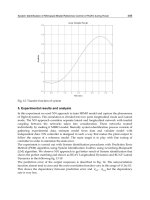
4. Result and Analysis
Figure 19 below shows offline EKF SLAM results using data logged by a robot. The
experiment was conducted inside a room of 900 cm x 720cm dimension with a few obstacles.
Using an EKF-SLAM algorithm which takes data information (corners locations &
odometry); a map of the room was developed. Corner features were extracted from the laser
data. To initialize the mapping process, the robot’s starting position was taken reference. In
figure 19 below, the top left corner is a map drawn using odometry; predictably the map is
skewed because of accumulation of errors. The top middle picture is an environment drawn
using EKF SLAM map (corners locations). The corners were extracted using an algorithm
we proposed, aimed at solving the possibility of mapping false corners. When a corner is re-
observed a Kalman filter update is done. This improves the overall position estimates of the
robot as well as the landmark. Consequently, this causes the confidence ellipse drawn
around the map (robot position and corners) to reduce in size (bottom left picture).


Fig. 18. In figure 8, two consecutive corner extraction process from the split and merge
algorithm maps one corner wrongly, while in contrast our corner extraction algorithm picks
out the same two corners and correctly associates them.


Fig. 19. EKF-SLAM simulation results showing map reconstruction (top right) of an office
space drawn from sensor data logged by the Meer Cat. When a corner is detected, its
position is mapped and a 2


confidence ellipse is drawn around the feature position. As
the number of observation of the same feature increase the confidence ellipse collapses (top
right). The bottom right picture depict x coordinate estimation error (blue) between 2


bounds (red). Perceptual inference

Expectedly, as the robot revisits its previous position, there is a major decrease in the ellipse,
indicating robot’s high perceptual inference of its position. The far top right picture shows a
reduction in ellipses around robot position. The estimation error is with the 2

, indicating
consistent results, bottom right picture. During the experiment, an extra laser sensor was
Feature extraction: techniques for landmark based navigation system 371
Compatibility Nearest Neighbour. Of the map features that satisfy IC, ICNN chooses one
with the smallest Mahalanobis distance (Castellanos, J.A et al. 2006).

3.6 Consistency of EKF-SLAM
EKF-SLAM consistency or lack of was discussed in (Castellanos, J.A et al. 2006), (Newman,
P.M. (1999), (Cooper, A.J, 2005), and (Castellanos, J.A et al. 2006), It is a non-linear problem
hence it is necessary to check if it is consistent or not. This can be done by analysing the
errors. The filter is said to be unbiased if the Expectation of the actual state estimation error,
( )k

X satisfies the following equation:

[ ] 0E X


(56)

  
( ) ( ) ( | 1)
T
E k k k k
 


 
 
 
X X P (57)
where the actual state estimation error is given by:


( ) ( ) ( | 1)k k k k

 

X X X
(58)

( | 1)k k P is the state error covariance. Equation (57) means that the actual mean square
error matches the state covariance. When the ground truth solution for the state variables is
available, a chi-squared test can be applied on the normalised estimation error squared to
check for filter consistency.





 


1
( ) ( | 1) ( )
T
k k k k


 
X P X
2
,1
d



 (59)

where DOF is equal to the state dimension


)(dim kxd

and


1 is the desired confidence
level. In most cases ground truth is not available, and consistency of the estimation is
checked using only measurements that satisfy the innovation test:

1 2
,1
( ) ( )
T
ij ij ij d
k k




v S v
(60)
Since the innovation term depends on the data association hypothesis, this process becomes
critical in maintaining a consistent estimation of the environment map.

4. Result and Analysis
Figure 19 below shows offline EKF SLAM results using data logged by a robot. The
experiment was conducted inside a room of 900 cm x 720cm dimension with a few obstacles.
Using an EKF-SLAM algorithm which takes data information (corners locations &
odometry); a map of the room was developed. Corner features were extracted from the laser
data. To initialize the mapping process, the robot’s starting position was taken reference. In
figure 19 below, the top left corner is a map drawn using odometry; predictably the map is
skewed because of accumulation of errors. The top middle picture is an environment drawn
using EKF SLAM map (corners locations). The corners were extracted using an algorithm
we proposed, aimed at solving the possibility of mapping false corners. When a corner is re-
observed a Kalman filter update is done. This improves the overall position estimates of the
robot as well as the landmark. Consequently, this causes the confidence ellipse drawn
around the map (robot position and corners) to reduce in size (bottom left picture).

Fig. 18. In figure 8, two consecutive corner extraction process from the split and merge
algorithm maps one corner wrongly, while in contrast our corner extraction algorithm picks
out the same two corners and correctly associates them.


Fig. 19. EKF-SLAM simulation results showing map reconstruction (top right) of an office
space drawn from sensor data logged by the Meer Cat. When a corner is detected, its
position is mapped and a 2

confidence ellipse is drawn around the feature position. As
the number of observation of the same feature increase the confidence ellipse collapses (top
right). The bottom right picture depict x coordinate estimation error (blue) between 2


bounds (red). Perceptual inference

Expectedly, as the robot revisits its previous position, there is a major decrease in the ellipse,
indicating robot’s high perceptual inference of its position. The far top right picture shows a
reduction in ellipses around robot position. The estimation error is with the 2

, indicating
consistent results, bottom right picture. During the experiment, an extra laser sensor was
Sensor Fusion and Its Applications372
user to track the robot position, this provided absolute robot position. An initial scan of the
environment (background) was taken prior by the external sensor. A simple matching is
then carried out to determine the pose of the robot in the background after exploration.
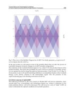
Figure 7 below shows that as the robot close the loop, the estimated path and the true are
almost identical, improving the whole map in the process.

-4 -3 -2 -1 0 1 2 3
-1
0
1
2
3
4
5
SLAM vs Abolute Position
[m]
[m]
SLAM
Abolute Position
termination position
start

Fig. 20. The figure depicts that as the robot revisits its previous explored regions; its
positional perception is high. This means improved localization and mapping, i.e. improved
SLAM output.

5. Conclusion and future work
In this paper we discussed the results of an EKF SLAM using real data logged and
computed offline. One of the most important parts of the SLAM process is to accurately map
the environment the robot is exploring and localize in it. To achieve this however, is
depended on the precise acquirement of features extracted from the external sensor. We
looked at corner detection methods and we proposed an improved version of the method
discussed in section 2.1.1. It transpired that methods found in the literature suffer from high
computational cost. Additionally, there are susceptible to mapping ‘ghost corners’ because
of underlying techniques, which allows many computations to pass as corners. This has a

major implication on the solution of SLAM; it can lead to corrupted map and increase
computational cost. This is because EKF-SLAM’s computational complexity is quadratic the
number of landmarks in the map, this increased computational burden can preclude real-
time operation. The corner detector we developed reduces the chance of mapping dummy
corners and has improved computation cost. This offline simulation with real data has
allowed us to test and validate our algorithms. The next step will be to test algorithm
performance in a real time. For large indoor environments, one would employ a try a
regression method to fit line to scan data. This is because corridors will have numerous
possible corners while it will take a few lines to describe the same space.

6. Reference
Bailey, T and Durrant-Whyte, H. (2006), Simultaneous Localisation and Mapping (SLAM):
Part II State of the Art. Tim. Robotics and Automation Magazine, September.
Castellanos, J.A., Neira, J., and Tard´os, J.D. (2004) Limits to the consistency of EKF-based
SLAM. In IFAC Symposium on Intelligent Autonomous Vehicles.
Castellanos, J.A.; Neira, J.; Tardos, J.D. (2006). Map Building and SLAM Algorithms,
Autonomous Mobile Robots: Sensing, Control, Decision Making and Applications, Lewis,
F.L. & Ge, S.S. (eds), 1st edn, pp 335-371, CRC, 0-8493-3748-8, New York, USA
Collier, J, Ramirez-Serrano, A (2009)., "Environment Classification for Indoor/Outdoor
Robotic Mapping," crv, Canadian Conference on Computer and Robot Vision , pp.276-
283.
Cooper, A.J. (2005). A Comparison of Data Association Techniques for Simultaneous
Localisation and Mapping, Masters Thesis, Massachusets Institute of Technology
Crowley, J. (1989). World modeling and position estimation for a mobile robot using
ultrasound ranging. In Proc. of the IEEE Int. Conf. on Robotics & Automation (ICRA).
Duda, R. O. and Hart, P. E. (1972) "Use of the Hough Transformation to Detect Lines and
Curves in Pictures," Comm. ACM, Vol. 15, pp. 11–15 ,January.
Durrant-Whyte, H and Bailey, T. (2006). Simultaneous Localization and Mapping (SLAM): Part I
The Essential Algorithms, Robotics and Automation Magazine.
Einsele, T. (2001) "Localization in indoor environments using a panoramic laser range

finder," Ph.D. dissertation, Technical University of München, September.
Hough ,P.V.C., Machine Analysis of Bubble Chamber Pictures. (1959). Proc. Int. Conf. High
Energy Accelerators and Instrumentation.
Li, X. R. and Jilkov, V. P. (2003). Survey of Maneuvering Target Tracking.Part I: Dynamic
Models. IEEE Trans. Aerospace and Electronic Systems, AES-39(4):1333.1364, October.
Lu, F. and Milios, E.E (1994). Robot pose estimation in unknown environments by matching
2D range scans. In Proc. of the IEEE Computer Society Conf. on Computer Vision and
Pattern Recognition (CVPR), pages 935–938.
Mathpages, “Perpendicular regression of a line”
(2010-04-23)
Mendes, A., and Nunes, U. (2004)"Situation-based multi-target detection and tracking with
laser scanner in outdoor semi-structured environment", IEEE/RSJ Int. Conf. on
Systems and Robotics, pp. 88-93.
Moutarlier, P. and Chatila, R. (1989a). An experimental system for incremental environment
modelling by an autonomous mobile robot. In ISER.
Moutarlier, P. and Chatila, R. (1989b). Stochastic multisensory data fusion for mobile robot
location and environment modelling. In ISRR ).
Feature extraction: techniques for landmark based navigation system 373
user to track the robot position, this provided absolute robot position. An initial scan of the
environment (background) was taken prior by the external sensor. A simple matching is
then carried out to determine the pose of the robot in the background after exploration.
Figure 7 below shows that as the robot close the loop, the estimated path and the true are
almost identical, improving the whole map in the process.

-4 -3 -2 -1 0 1 2 3
-1
0
1
2
3

4
5
SLAM vs Abolute Position
[m]
[m]
SLAM
Abolute Position
termination position
start

Fig. 20. The figure depicts that as the robot revisits its previous explored regions; its
positional perception is high. This means improved localization and mapping, i.e. improved
SLAM output.

5. Conclusion and future work
In this paper we discussed the results of an EKF SLAM using real data logged and
computed offline. One of the most important parts of the SLAM process is to accurately map
the environment the robot is exploring and localize in it. To achieve this however, is
depended on the precise acquirement of features extracted from the external sensor. We
looked at corner detection methods and we proposed an improved version of the method
discussed in section 2.1.1. It transpired that methods found in the literature suffer from high
computational cost. Additionally, there are susceptible to mapping ‘ghost corners’ because
of underlying techniques, which allows many computations to pass as corners. This has a
major implication on the solution of SLAM; it can lead to corrupted map and increase
computational cost. This is because EKF-SLAM’s computational complexity is quadratic the
number of landmarks in the map, this increased computational burden can preclude real-
time operation. The corner detector we developed reduces the chance of mapping dummy
corners and has improved computation cost. This offline simulation with real data has
allowed us to test and validate our algorithms. The next step will be to test algorithm
performance in a real time. For large indoor environments, one would employ a try a

regression method to fit line to scan data. This is because corridors will have numerous
possible corners while it will take a few lines to describe the same space.

6. Reference
Bailey, T and Durrant-Whyte, H. (2006), Simultaneous Localisation and Mapping (SLAM):
Part II State of the Art. Tim. Robotics and Automation Magazine, September.
Castellanos, J.A., Neira, J., and Tard´os, J.D. (2004) Limits to the consistency of EKF-based
SLAM. In IFAC Symposium on Intelligent Autonomous Vehicles.
Castellanos, J.A.; Neira, J.; Tardos, J.D. (2006). Map Building and SLAM Algorithms,
Autonomous Mobile Robots: Sensing, Control, Decision Making and Applications, Lewis,
F.L. & Ge, S.S. (eds), 1st edn, pp 335-371, CRC, 0-8493-3748-8, New York, USA
Collier, J, Ramirez-Serrano, A (2009)., "Environment Classification for Indoor/Outdoor
Robotic Mapping," crv, Canadian Conference on Computer and Robot Vision , pp.276-
283.
Cooper, A.J. (2005). A Comparison of Data Association Techniques for Simultaneous
Localisation and Mapping, Masters Thesis, Massachusets Institute of Technology
Crowley, J. (1989). World modeling and position estimation for a mobile robot using
ultrasound ranging. In Proc. of the IEEE Int. Conf. on Robotics & Automation (ICRA).
Duda, R. O. and Hart, P. E. (1972) "Use of the Hough Transformation to Detect Lines and
Curves in Pictures," Comm. ACM, Vol. 15, pp. 11–15 ,January.
Durrant-Whyte, H and Bailey, T. (2006). Simultaneous Localization and Mapping (SLAM): Part I
The Essential Algorithms, Robotics and Automation Magazine.
Einsele, T. (2001) "Localization in indoor environments using a panoramic laser range
finder," Ph.D. dissertation, Technical University of München, September.
Hough ,P.V.C., Machine Analysis of Bubble Chamber Pictures. (1959). Proc. Int. Conf. High
Energy Accelerators and Instrumentation.
Li, X. R. and Jilkov, V. P. (2003). Survey of Maneuvering Target Tracking.Part I: Dynamic
Models. IEEE Trans. Aerospace and Electronic Systems, AES-39(4):1333.1364, October.
Lu, F. and Milios, E.E (1994). Robot pose estimation in unknown environments by matching
2D range scans. In Proc. of the IEEE Computer Society Conf. on Computer Vision and

Pattern Recognition (CVPR), pages 935–938.
Mathpages, “Perpendicular regression of a line”
/>. (2010-04-23)
Mendes, A., and Nunes, U. (2004)"Situation-based multi-target detection and tracking with
laser scanner in outdoor semi-structured environment", IEEE/RSJ Int. Conf. on
Systems and Robotics, pp. 88-93.
Moutarlier, P. and Chatila, R. (1989a). An experimental system for incremental environment
modelling by an autonomous mobile robot. In ISER.
Moutarlier, P. and Chatila, R. (1989b). Stochastic multisensory data fusion for mobile robot
location and environment modelling. In ISRR ).
Sensor Fusion and Its Applications374
Newman, P.M. (1999). On the structure and solution of the simultaneous localization and
mapping problem. PhD Thesis, University of Sydney.
Newman, P. (2006) EKF Based Navigation and SLAM, SLAM Summer School.
Pfister, S.T., Roumeliotis, S.I., and Burdick, J.W. (2003). Weighted line fitting algorithms for
mobile robot map building and efficient data representation. In Proc. of the IEEE Int.
Conf. on Robotics & Automation (ICRA).
Roumeliotis S.I. and Bekey G.A. (2000). SEGMENTS: A Layered, Dual-Kalman filter
Algorithm for Indoor Feature Extraction. In Proc. IEEE/RSJ International Conference
on Intelligent Robots and Systems, Takamatsu, Japan, Oct. 30 - Nov. 5, pp.454-461.
Smith, R., Self, M. & Cheesman, P. (1985). On the representation and estimation of spatial
uncertainty. SRI TR 4760 & 7239.
Smith, R., Self, M. & Cheesman, P. (1986). Estimating uncertain spatial relationships in
robotics, Proceedings of the 2nd Annual Conference on Uncertainty in Artificial
Intelligence, (UAI-86), pp. 435–461, Elsevier Science Publishing Company, Inc., New
York, NY.
Spinello, L. (2007). Corner extractor, Institute of Robotics and Intelligent Systems, Autonomous
Systems Lab,
/>,
ETH Zürich

Thorpe, C. and Durrant-Whyte, H. (2001). Field robots. In ISRR’.
Thrun, S., Koller, D., Ghahmarani, Z., and Durrant-Whyte, H. (2002) Slam updates require
constant time. Tech. rep., School of Computer Science, Carnegie Mellon University
Williams S.B., Newman P., Dissanayake, M.W.M.G., and Durrant-Whyte, H. (2000.).
Autonomous underwater simultaneous localisation and map building. Proceedings
of IEEE International Conference on Robotics and Automation, San Francisco, USA, pp.
1143-1150,
Williams, S.B.; Newman, P.; Rosenblatt, J.; Dissanayake, G. & Durrant-Whyte, H. (2001).
Autonomous underwater navigation and control, Robotica, vol. 19, no. 5, pp. 481-
496.
Sensor Data Fusion for Road Obstacle Detection: A Validation Framework 375
Sensor Data Fusion for Road Obstacle Detection: A Validation Framework
Raphaël Labayrade, Mathias Perrollaz, Dominique Gruyer and Didier Aubert
X

Sensor Data Fusion for Road
Obstacle Detection: A Validation Framework

Raphaël Labayrade
1
, Mathias Perrollaz
2
,
Dominique Gruyer
2
and Didier Aubert
2

1
ENTPE (University of Lyon)

France
2
LIVIC (INRETS-LCPC)
France

1. Introduction
Obstacle detection is an essential task for autonomous robots. In particular, in the context of
Intelligent Transportation Systems (ITS), vehicles (cars, trucks, buses, etc.) can be considered
as robots; the development of Advance Driving Assistance Systems (ADAS), such as
collision mitigation, collision avoidance, pre-crash or Automatic Cruise Control, requires
that reliable road obstacle detection systems are available. To perform obstacle detection,
various approaches have been proposed, depending on the sensor involved: telemeters like
radar (Skutek et al., 2003) or laser scanner (Labayrade et al., 2005; Mendes et al., 2004),
cooperative detection systems (Griffiths et al., 2001; Von Arnim et al., 2007), or vision
systems. In this particular field, monocular vision generally exploits the detection of specific
features like edges, symmetry (Bertozzi et al., 2000), color (Betke & Nguyen, 1998)
(Yamaguchi et al., 2006) or even saliency maps (Michalke et al., 2007). Anyway, most
monocular approaches suppose recognition of specific objects, like vehicles or pedestrians,
and are therefore not generic. Stereovision is particularly suitable for obstacle detection
(Bertozzi & Broggi, 1998; Labayrade et al., 2002; Nedevschi et al., 2004; Williamson, 1998),
because it provides a tri-dimensional representation of the road scene. A critical point about
obstacle detection for the aimed automotive applications is reliability: the detection rate
must be high, while the false detection rate must remain extremely low. So far, experiments
and assessments of already developed systems show that using a single sensor is not
enough to meet these requirements: due to the high complexity of road scenes, no single
sensor system can currently reach the expected 100% detection rate with no false positives.
Thus, multi-sensor approaches and fusion of data from various sensors must be considered,
in order to improve the performances. Various fusion strategies can be imagined, such as
merging heterogeneous data from various sensors (Steux et al., 2002). More specifically,
many authors proposed cooperation between an active sensor and a vision system, for

instance a radar with mono-vision (Sugimoto et al., 2004), a laser scanner with a camera
(Kaempchen et al., 2005), a stereovision rig (Labayrade et al., 2005), etc. Cooperation
between mono and stereovision has also been investigated (Toulminet et al., 2006).
16
Sensor Fusion and Its Applications376

Our experiments in the automotive context showed that using specifically a sensor to
validate the detections provided by another sensor is an efficient scheme that can lead to a
very low false detection rate, while maintaining a high detection rate. The principle consists
to tune the first sensor in order to provide overabundant detections (and not to miss any
plausible obstacles), and to perform a post-process using the second sensor to confirm the
existence of the previously detected obstacles. In this chapter, such a validation-based
sensor data fusion strategy is proposed, illustrated and assessed.

The chapter is organized as follows: the validation framework is presented in Section 2. The
next sections show how this framework can be implemented in the case of two specific
sensors, i.e. a laser scanner aimed at providing hypothesis of detections, and a stereovision
rig aimed at validating these detections. Section 3 deals with the laser scanner raw data
processing: 1) clustering of lasers points into targets; and 2) tracking algorithm to estimate
the dynamic state of the objects and to monitor their appearance and disappearance. Section
4 is dedicated to the presentation of the stereovision sensor and of the validation criteria. An
experimental evaluation of the system is given. Eventually, section 5 shows how this
framework can be implemented with other kinds of sensors; experimental results are also
presented. Section 6 concludes.

2. Overview of the validation framework
Multi-sensor combination can be an efficient way to perform robust obstacle detection. The
strategy proposed in this chapter is a collaborative approach illustrated in Fig. 1. A first
sensor is supposed to provide hypotheses of detection, denoted ‘targets’ in the reminder of
the chapter. The sensor is tuned to perform overabundant detection and to avoid missing

plausible obstacles. Then a post process, based on a second sensor, is performed to confirm
the existence of these targets. This second step is aimed at ensuring the reliability of the
system by discarding false alarms, through a strict validation paradigm.











Fig. 1. Overview of the validation framework: a first sensor outputs hypothesis of detection.
A second sensor validates those hypothesis.

The successive steps of the validation framework are as follows. First, a volume of interest
(VOI) surrounding the targets is built in the 3D space in front of the equipped vehicle, for
each target provided by the first sensor. Then, the second sensor focuses on each VOI, and
evaluates criteria to validate the existence of the targets. The only requirement for the first

sensor is to provide localized targets with respect to the second sensor, so that VOI can be
computed.
In the next two sections, we will show how this framework can be implemented for two
specific sensors, i.e. a laser scanner, and a stereovision rig; section 5 will study the case of an
optical identification sensor as first sensor, along with a stereovision rig as second sensor. It
is convenient to assume that all the sensors involved in the fusion scheme are rigidly linked
to the vehicle frame, so that, after calibration, they can all refer to a common coordinate
system. For instance, Fig. 2 presents the various sensors taken into account in this chapter,

referring to the same coordinate system.
















Fig. 2. The different sensors used located in the same coordinate system R
a
.

3. Hypotheses of detection obtained from the first sensor: case of a 2D laser
scanner
The laser scanner taken into account in this chapter is supposed to be mounted at the front
of the equipped vehicle so that it can detect obstacles on its trajectory. This laser scanner
provides a set of laser points on the scanned plane: each laser point is characterized by an
incidence angle and a distance which corresponds to the distance of the nearest object in this
direction. Fig. 4. shows a (X, -Y) projection of the laser points into the coordinate system
linked to the laser scanner and illustrated in Fig. 2.

3.1 Dynamic clustering
From the raw data captured with the laser scanner, a set of clusters must be built, each
cluster corresponding to an object in the observed scene (a so-called ‘target’). Initially, the
first laser point defines the first cluster. For all other laser points, the goal is to know
whether they are a member of the existent cluster or whether they belong to a new cluster.
In the literature, a large set of distance functions can be found for this purpose.



Sensor Data Fusion for Road Obstacle Detection: A Validation Framework 377

Our experiments in the automotive context showed that using specifically a sensor to
validate the detections provided by another sensor is an efficient scheme that can lead to a
very low false detection rate, while maintaining a high detection rate. The principle consists
to tune the first sensor in order to provide overabundant detections (and not to miss any
plausible obstacles), and to perform a post-process using the second sensor to confirm the
existence of the previously detected obstacles. In this chapter, such a validation-based
sensor data fusion strategy is proposed, illustrated and assessed.

The chapter is organized as follows: the validation framework is presented in Section 2. The
next sections show how this framework can be implemented in the case of two specific
sensors, i.e. a laser scanner aimed at providing hypothesis of detections, and a stereovision
rig aimed at validating these detections. Section 3 deals with the laser scanner raw data
processing: 1) clustering of lasers points into targets; and 2) tracking algorithm to estimate
the dynamic state of the objects and to monitor their appearance and disappearance. Section
4 is dedicated to the presentation of the stereovision sensor and of the validation criteria. An
experimental evaluation of the system is given. Eventually, section 5 shows how this
framework can be implemented with other kinds of sensors; experimental results are also
presented. Section 6 concludes.

2. Overview of the validation framework
Multi-sensor combination can be an efficient way to perform robust obstacle detection. The
strategy proposed in this chapter is a collaborative approach illustrated in Fig. 1. A first
sensor is supposed to provide hypotheses of detection, denoted ‘targets’ in the reminder of
the chapter. The sensor is tuned to perform overabundant detection and to avoid missing
plausible obstacles. Then a post process, based on a second sensor, is performed to confirm
the existence of these targets. This second step is aimed at ensuring the reliability of the
system by discarding false alarms, through a strict validation paradigm.











Fig. 1. Overview of the validation framework: a first sensor outputs hypothesis of detection.
A second sensor validates those hypothesis.

The successive steps of the validation framework are as follows. First, a volume of interest
(VOI) surrounding the targets is built in the 3D space in front of the equipped vehicle, for
each target provided by the first sensor. Then, the second sensor focuses on each VOI, and
evaluates criteria to validate the existence of the targets. The only requirement for the first

sensor is to provide localized targets with respect to the second sensor, so that VOI can be
computed.
In the next two sections, we will show how this framework can be implemented for two

specific sensors, i.e. a laser scanner, and a stereovision rig; section 5 will study the case of an
optical identification sensor as first sensor, along with a stereovision rig as second sensor. It
is convenient to assume that all the sensors involved in the fusion scheme are rigidly linked
to the vehicle frame, so that, after calibration, they can all refer to a common coordinate
system. For instance, Fig. 2 presents the various sensors taken into account in this chapter,
referring to the same coordinate system.
















Fig. 2. The different sensors used located in the same coordinate system R
a
.

3. Hypotheses of detection obtained from the first sensor: case of a 2D laser
scanner
The laser scanner taken into account in this chapter is supposed to be mounted at the front
of the equipped vehicle so that it can detect obstacles on its trajectory. This laser scanner

provides a set of laser points on the scanned plane: each laser point is characterized by an
incidence angle and a distance which corresponds to the distance of the nearest object in this
direction. Fig. 4. shows a (X, -Y) projection of the laser points into the coordinate system
linked to the laser scanner and illustrated in Fig. 2.

3.1 Dynamic clustering
From the raw data captured with the laser scanner, a set of clusters must be built, each
cluster corresponding to an object in the observed scene (a so-called ‘target’). Initially, the
first laser point defines the first cluster. For all other laser points, the goal is to know
whether they are a member of the existent cluster or whether they belong to a new cluster.
In the literature, a large set of distance functions can be found for this purpose.