Wind Power Impact on Power System Dynamic Part 15 doc
Bạn đang xem bản rút gọn của tài liệu. Xem và tải ngay bản đầy đủ của tài liệu tại đây (2 MB, 35 trang )
Power Characteristics of Compound Microgrid Composed from PEFC and Wind Power Generation
473
period of step input of 6 kW and 8 kW for 3.9 seconds. If a wind power generator is
connected to the micro-grid, many fluctuations in the system response characteristics will
occur in a short period. If the power produced by wind power generation is supplied to the
micro-grid, the dynamic characteristics of power of the micro-grid will be influenced. Figure
8 (b) shows the analysis result of the response error corresponding to Figure 8 (a). If wind
power generator is connected to the grid, the response error will become large as the load of
the grid becomes small. It is expected that the power range of the fluctuation of the micro-
grid will increase as the output of the wind power generation grows. Therefore, when the
load of a micro-grid is small compared with the output of wind power generator, the power
supply of the independent micro-grid becomes unstable.
5.2 Load response characteristics of cold region houses
Figure 9 (a) shows the power demand pattern of a micro-grid formed from ten individual
houses in Sapporo in Japan, and assumes a representative day in February (Narita, 1996).
This power demand pattern is the average value of each hour, and the sampling time of
analyses and the assumption time are written together on the horizontal axis. As a base load
of the power demand pattern shown in Fig. 9 (a), F/C (0) is considered as operation of 2.5
kW constant load. Figure 9 (b) and (c) are the power demand patterns when adding load
fluctuations (±1 kW and ±3 kW) to Fig. 9 (a) at random. The variation of the load was
decided at random within the limits of the range of fluctuation for every sampling time.
Fig. 9. 480s demand model for 10 houses in February in Sapporo
Wind Power
474
Figure 10 shows the response results of F/C (0) to F/C (6) when wind power generation is
connected to the micro-grid and the power load has ±1 kW fluctuations. F/C (0) assumed
operation with 2.5 kW constant output, with the result that the response of F/C (0) is much
less than 2.5 kW in less than the sampling time of 100 s as shown in Figure 10 (a). This
reason is because F/C (0) was less than 2.5 kW with the power of wind power generation.
Although the micro-grid assumed in this paper controlled the number of operations of F/C
(1) to F/C (7) depending on the magnitude of the load, since the power supply of wind
power generation existed, there was no operating time of F/C (7).
Fig. 10. Response results of each fuel cell
5.3 Power generation efficiency
Figure 11 shows the analysis results of the average power generation efficiency of fuel cell
systems for every sampling time. The average efficiency of a fuel cell system is the value
averaging the efficiency of F/C (0) to F/C (7) operated at each sampling time. However, the
fuel cell system to stop is not included in average power generation efficiency. The average
power generation efficiency of Figure 11 (a) is 13.4%, and Figure 10 (b) shows 14.3%. The
difference in average efficiency occurs in the operating point of a fuel cell system shifting to
the efficient side, when load fluctuations are added to the micro-grid. Thus, if load
fluctuations are added to the micro-grid, compared with no load fluctuations, the load factor
of the fuel cell system shown in Figure 4 will increase.
Power Characteristics of Compound Microgrid Composed from PEFC and Wind Power Generation
475
Fig. 11. Results of micro-grid average efficiency
Fig. 12. Results of efficiency for each fuel cell
Wind Power
476
Figure 12 shows the power generation efficiency of each fuel cell in the case of connecting
wind power generation to the micro-grid of ±1.0kW of load fluctuation. F/C (0) operated
corresponding to a base load has maximum power generation efficiency at all sampling
times. Since the number of operations of a fuel cell is controlled by the magnitude of the
load added to the micro-grid, the operating time falls in the order of F/C (1) to F/C (6).
Moreover, there is no time to operate F/C (7) in this operating condition.
The relation between the range of fluctuation of the power load and the existence of wind
power generation, and the amount of electricity demand of a representative day is shown
Fig. 13. When the load fluctuation of the power is large, although the power demand
amount of the micro-grid on a representative day increases slightly, it is less than 2%.
Moreover, when installing wind power generation, the power demand amount of the micro-
grid of a representative day decreases compared with the case of not installing. This
decrement is almost equal to the value that integrated the power (average of 0.75 kW)
supplied to a grid by the wind power generation of Fig. 4 (b).
Fig. 13. Amount of 480s demand model with power fluctuation and wind power generation
Figure 14 shows the range of fluctuation of power load and the existence of wind power
generation, and the relation to city gas consumption on a representative day of the micro-
grid. If the range of fluctuation of the power load becomes large, city gas consumption will
decrease. This is because electric power supply cannot follow the load fluctuations of the
micro-grid if the range of fluctuation of the power load is large. Moreover, in ±3 kW of load
fluctuation, some loads become zero (it sees from 20s to 100s of sampling times) and city gas
consumption lowers. In ±3 kW of load fluctuation of the power, it is expected that the power
of a micro-grid is unstable and introduction to a real system is not suitable.
Power Characteristics of Compound Microgrid Composed from PEFC and Wind Power Generation
477
Fig. 14. Analysis result of town gas consumption for 480s demand model with power
fluctuation and wind power generation
6. Conclusions
A 2.5 kW fuel cell was installed in a house linked to a micro-grid, operation corresponding
to a base load was conducted, and the dynamic characteristics of the grid when installing a 1
kW fuel cell system in seven houses were investigated by numerical analysis. A wind power
generator outputted to a micro-grid at random within 1.5 kW was installed, and the
following conclusions were obtained.
1. Although the settling time (time to converge on ±5% of the target output) of the micro-
grid differs with the magnitude of the load, and the parameters of the controller, it is
about 4 seconds.
2. When connecting a wind power generator to the micro-grid, the instability of the power
of the grid due to supply-and-demand difference is an issue. This issue is remarkable
when the load of an independent micro-grid is small compared to the production of
electricity of unstable wind power generation.
3. When wind power equipment is connected to the micro-grid with load fluctuation, the
operating point of the fuel cell system may shift and power generation efficiency may
improve.
7. Acknowledgements
This work was partially supported by a Grant-in-Aid for Scientific Research(C) from the
JSPS.KAKENHI (17510078).
8. Nomenclature
Act : ‘’ If “ action
Wind Power
478
Act_FC : Each fuel cell operation
F /C : Fuel cell
h
: Capacity of generation W
I
: Integral parameter
P
: Proportionality parameter
PI : Proportion integration control
u
: Power load of a micro-grid W
ν
: Power output W
9. References
Abu-Sharkh, S.; Arnold, R. J.; Kohler, J.; Li, R.; Markvart, T.; Ross, J. N.; Steemers, K.; Wilson,
P. & Yao, R. (2006). Can microgrids make a major contribution to UK energy
supply?. Renewable and Sustainable Energy Reviews, Vol. 10, No. 2, pp. 78-127.
Carlos, A. & Hernandez, A. (2005). Fuel consumption minimization of a microgrid. IEEE
Transactions on Industry Applications, Vol. 41, No. 3, pp. 673- 681.
Ibe, S.; Shinke, N.; Takami, S.; Yasuda, Y.; Asatsu, H. & Echigo, M. (2002). Development of
Fuel Processor for Residential Fuel Cell Cogeneration System, Proc. 21
th
Annual
Meeting of Japan Society of Energy and Resources, pp. 493-496, Osaka, June 12-13, ed.,
Abe, K. (in Japanese)
Kyoto Denkiki Co., Ltd. A system connection inverter catalog and an examination data sheet, 2001.
Lindstrom, B. & Petterson, L. (2003). Development of a methanol fuelled reformer for fuel
cell applications, J. Power Source, Vol. 118, pp. 71-78.
Nagano, S. (2002). Plate-Type Methanol Steam Reformer Using New Catalytic Combustion
for a Fuel Cell. Proceedings of SAE Technical Paper Series, Automotive Eng. pp. 10.
Narita, K. (1996). The Research on Unused Energy of the Cold Region City and Utilization
for the District Heat and Cooling. Ph.D. thesis, Hokkaido University, Sapporo. (in
Japanese)
Obara, S. & Kudo, K. (2005). Installation Planning of Small-Scale Fuel Cell Cogeneration in
Consideration of Load Response Characteristics (Load Response Characteristics of
Electric Power Output). Transactions of the Japan Society of Mechanical Engineers,
Series B; Vol. 71, No.706, pp. 1678-1685. (in Japanese)
Obara, S. & Kudo, K. (2005). Study on Small-Scale Fuel Cell Cogeneration System with
Methanol Steam Reforming Considering Partial Load and Load Fluctuation.
Transactions of the ASME, Journal of Energy Resources Technology, Vol. 127, pp. 265-
271.
Oda, K.; Sakamoto, S.; Ueda, M.; Fuji, A. & Ouki, T. (1999). A Small-Scale Reformer for Fuel
Cell Application. Sanyo Technical Review, Vol. 31, No. 2, pp. 99-106, Sanyo Electric
Co., Ltd., Tokyo, Japan. (in Japanese)
Robert, H. (2004). Microgrid: A conceptual solution. Proceedings of the 35th Annual IEEE
Power Electronics Specialists Conference, Vol. 6, pp. 4285-4290.
Takeda, Y.; Iwasaki, Y.; Imada, N. & Miyata, T. (2004). Development of Fuel Processor for
Rapid Start-up, Proc. 20
th
Energy System Economic and Environment Conference,
Tokyo, January 29-30, ed., K. Kimura, pp. 343-344. (in Japanese)
21
Large Scale Integration of Wind Power
in Thermal Power Systems
Lisa Göransson and Filip Johnsson
Chalmers University of Technology
Sweden
1. Introduction
This chapter discusses and compares different modifications of wind-thermal electricity
generation systems, which have been suggested for the purpose of handling variations in
wind power generation. Wind power is integrated into our electricity generation systems to
decrease the amount of carbon dioxide emissions associated with the generation of
electricity as well as to enhance security of supply. However, the electricity generated by
wind varies over time whereas thermal units are most efficient if run continuously at rated
power. Thus, depending on the characteristics of the wind-thermal system, part of the
decrease in emissions realized by wind power is offset by a reduced efficiency in operation
of the thermal units as a result of the variations in generation from wind. This chapter
discusses the extent to which it is possible to improve the ability of a wind-thermal system
to manage such variations.
The first part of the chapter deals with the nature of the variations present in a wind-thermal
power system, i.e. variations in load and wind power generation, and the impact of these
variations on the thermal units in the system. The second part of the chapter investigates
and evaluates options to moderate variations from wind power by integrating different
types of storage such as pumped hydro power, compressed air energy storage, flow
batteries and sodium sulphur batteries. In addition, the option of interconnecting power
systems in a so called “supergrid” is discussed as well as to moderate wind power
variations by managing the load on the thermal units through charging and discharging of
plug-in hybrid electric vehicles.
Data from the power system of western Denmark is used to illustrate various aspects
influencing the ability of a power system to accommodate wind power. Western Denmark
was chosen primarily due to its current high wind power grid penetration level (24% in 2005
(Ravn 2001; Eltra 2005)) and that data from western Denmark is easily accessible through
Energinet (2006).
2. Impact of wind power variations on thermal plants
The power output of a single wind turbine can vary rapidly between zero and full
production. However, since the power generated by one turbine is small relative to the
capacity of a thermal unit, such fluctuations have negligible impact on the generation
pattern of the thermal units in the overall system. With several wind farms in a power
Wind Power
480
system, the total possible variation in power output can add up to capacities corresponding
to the thermal units and influence the overall generation pattern. At times of low wind
speeds, some thermal unit might for example need to be started. The power output of the
aggregated wind power is, however, quite different from the power output of a single
turbine. Wind speeds depend on weather patterns as well as the landscape around the wind
turbines (i.e. roughness of the ground, sea breeze etc.). Thus, the greater the difference in
weather patterns and environmental conditions between the locations of the wind turbines,
the lower the risk of correlation in power output. In a power system with geographically
dispersed wind farms, the effect of local environmental conditions on power output will be
reduced. Since it takes some time for a weather front to pass a region, the effect of weather
patterns will be delayed from one farm to another, and the alteration in aggregated power
output thus takes place over a couple of hours rather than instantaneously. This effect is
referred to as power smoothing (Manwell et al. 2005). Western Denmark is a typical
example of a region with dispersed wind power generation. The aggregated wind power
output for this region during one week in January can be found in Figure 1. As seen in
Figure 1, variations in the range of the capacity of thermal units do occur (e.g. between 90
hours and 100 hours the wind power generation decreases with 1 000MW), but the increase
or decrease in power over such range takes at least some hours (e.g. approximately 10 hours
for the referred to example ).
2.1 Variations in load and wind power generation
Figure 2 illustrates the variations in total load (electricity consumption) in western Denmark
during the same week as shown in Figure 1. As seen, the amplitude of the wind power
variations at current wind power grid penetration (i.e. 24%) and the variations in load are
not much different. However, there are two aspects of wind power variations which make
these more complicated to manage than fluctuations in load; the unpredictability and the
irregularity. Since the total load variations are predictable, it is possible to plan the
scheduling of the thermal units to compensate for the load variations. The unpredictability
of wind power makes it difficult to accurately schedule units with long start-up times.
Variations in a system dominated by base load units create a need for what is here referred
to as moderator which is a unit in the power system with the ability to reallocate power in
time, such as a storage unit or import/export capacity. Since the total load variations are
regular, to manage these a moderator would only need to have “storage” capacity which
can displace one such variation at a time (i.e. absorb power for a maximum of 12 hours and
then deliver this power to the system). Due to the irregularity of wind power variations
“storage” capacities of a moderator for this application need to be more extensive than if
variations were regular.
For the thermal units it is obviously the aggregated impact of the wind power and the total
load which is of importance. The load on the thermal units (i.e. the total load reduced by the
wind power generation) will become both less predictable and less regular as wind power is
introduced to the system. In the Nordic countries, there is some correlation between wind
speeds and electric load in the summer, but no correlation of significance in winter time
(Holttinen 2005). However, a decrease/increase in wind power output might obviously
coincide with an increase/decrease in demand at any time of the year, resulting in large
variations in load on the thermal units. At times when wind power output is high and
demand is low, systems with wind power in the range of 20% grid penetration or higher
Large Scale Integration of Wind Power in Thermal Power Systems
481
might face situations where power generation exceeds demand (although this obviously
depends on the extent of the variations in load). Without a moderator in the system, which
can displace the excess power in time, some of the wind power generated will have to be
curtailed in such situations. With base load capacity in the system which has to run
continuously, situations where curtailment cannot be avoided will arise more frequently
1
.
0
500
1000
1500
2000
2500
0 20 40 60 80 100 120 140 160 180
Time of the week [hours]
Wind power generation [MW]
Fig. 1. Wind power generation in western Denmark during the first week in January 2005.
Source (Energinet 2006)
1500
2000
2500
3000
3500
4000
0 20 40 60 80 100 120 140 160 180
Time of the week [hours]
Total load [MW]
Fig. 2. Total load in western Denmark the first week in January 2005. Source (Energinet 2006)
2.2 Response to variations in wind power generation and electricity consumption
Variations in load in a wind-thermal power system that uses no active strategy for variation
management can be managed in three different ways;
• by part load operation of thermal units,
• by starting/stopping thermal units or
• by curtailing wind power.
The choice of variation management strategy depends on the properties of the thermal units
which are available for management (e.g. in order to choose to stop a unit it obviously has to
1
It should be pointed out that the Nordic system (Nordpool electricity market) of which
western Denmark is part, is special in the context of wind power integration, since
variations in wind power can, to a certain extent, be managed by hydropower (with large
reservoirs).
Wind Power
482
be running) and the duration of the variation. In a power system where cost is minimized,
the variation management strategy associated with the lowest cost is obviously chosen. If,
for example, the output of wind power and some large base load unit exceeds demand for
an hour, curtailment of wind power (or possibly some curtailment in combination with part
load of the thermal unit) might be the solution associated with the lowest total system cost.
If the same situation lasts for half a day, stopping the thermal unit might be preferable from
a cost minimizing perspective. To be able to take variation management decisions into
account in the dispatch of units, knowledge of the start-up and part load properties of the
thermal units is necessary.
Two aspects of the start-up of thermal units will have an immediate impact on the
scheduling of the units; the start-up time and the start-up cost. The start-up time is either
measured as the time it takes to warm up a unit before it reaches such a state that electricity
can be delivered to the grid (time for synchronization) or as the time before it delivers at
rated power (time until full production). In both cases, the start-up time ultimately depends
on the capacity of the unit, the power plant technology and the time during which the unit
has been idle. Small gas turbines have relatively short start-up times, in the range of 15
minutes, and large steam turbines have long start-up times, in the range of several hours. If
a large unit has been idle for a few hours, materials might still be warm and the start-up
time can be reduced. Table 1 presents the required start-up times of units in the Danish
power system.
The costs associated with starting a thermal unit are a result of the cost of the fuel required
during the warm-up phase and the accelerated component aging due to the stresses on the
plant from temperature changes. Lefton et al. (1995) have shown that the combined effect of
creep, due to base load operation, and fatigue, due to cycling (start-up/shutdown and load
following operation), can significantly reduce the lifetime of materials commonly used in
fossil fuel power plants in comparison to creep alone. They estimate the cycling costs (the
cost to stop and then restart a unit) of a conventional fossil power plant to $1 500-$500 000
per cycle (around EUR 1 170-400 000) with the range corresponding to differences in cycling
ability of different technologies and the duration of the stop. These costs include the cost of
increased maintenance, as well as an increase in total system costs due to lower availability
of cycled units, and an increase in engineering costs to adapt units to the new situation (i.e.
improve the cycling ability).
Table 1. Maximum allowed starting time for power plants in the Danish power system with
nominal maximum power above 25 MW. Source: (Energinet 2007).
One alternative to shutting down and restarting a thermal unit is to reduce the load in one
or several units. The load reduction in each unit is restricted by the maximum load turn-
down ratio. The minimum load level of a thermal unit depends on the power plant
technology and the fuel used in combustion units. The minimum load level on the Danish
Large Scale Integration of Wind Power in Thermal Power Systems
483
units range from 20% of rated power for gas- and oil-fired steam power plants to 70% of
rated power for waste power plants (Energinet 2007). Minimum load level of coal fired
power plants range from 35% to 50% of rated power depending on technology (Energinet
2007).
Running thermal units at part load is associated with an increase in costs and emissions per
unit of energy generated (i.e. per MWh), since the efficiency decreases with the load level.
The rate of the decrease in efficiency depends on the power plant technology and the level
to which the load is reduced. Figure 3 illustrates the relation between efficiency and load
level for three different thermal units. As shown in Figure 3, the rate of decrease in
efficiency is lower at high load levels than at low load levels. It is also shown that the rate of
decrease in efficiency is higher in the combined cycle plant (CC) than in the steam plant
(since gas turbines are sensitive to part load operation).
Fig. 3. Typical electric efficiency versus load level curves of different power plants. Source:
(Carraretto 2006)
Work with models of the power system of western Denmark suggests that wind power
variations introduce aspects that influence the competitiveness of the thermal units in the
power system relative to one another (Göransson & Johnsson 2009a). In general, simulations
show that an increase in the amount of wind power reduces the periods of constant
production and the duration of these periods. The capacity factor of units with low start-up
and turn down performance and high minimum load level (i.e. base load units) will
decrease more than the capacity factor of units with high start-up and turn down
performance and/or low minimum load level. This result might seem trivial. However, low
start-up and turn down performance and high minimum load levels are common properties
of units with low running costs designed for base load production. Thus, low running costs
compete against flexibility and in a system with significant wind power capacity, the unit
with the lowest running costs is not necessarily the unit which is run the most.
Figure 4 shows the capacity factors of the thermal units in the power system of western
Denmark at three different levels of wind power capacity (‘‘without wind’’, ‘‘current wind’’
corresponding to around 20% wind power grid penetration and ‘‘34% wind’’ with 34% wind
power grid penetration) from simulations of three weeks in July 2005 (Göransson &
Johnsson 2009a). As can be seen in Figure 4, the dominating trend is a decrease in import
and an increase in export as the wind power capacity in the system increases.
Wind Power
484
Start-up / turn down performance and minimum load level included
0
10
20
30
40
50
60
70
Enstedverket
Fynsver
ket
1
Fynsverket 2
N
o
rdj
yl
la
n
dsve
r
k
e
t
1
Nordjyllandsverket 2
Skerbe
ve
rket
St
u
dstr
u
p
ve
rket
1
St
u
dstrup
v
erket 2
Esbjergverket
Her
n
ing
e
verket
i
m
port
f
rom Sweden
i
mpor
t
f
rom
N
or
wa
y
import from Germany
export
to Swe
d
en
e
xpo
rt to
N
or
wa
y
e
xpor
t
to
G
er
ma
ny
wi
n
d
Capacity factor [%]
no wind
current wind
150% wind
Fig. 4. Simulated impact of variations in wind power generation on the capacity factor of
thermal units in western Denmark. For further details see (Göransson & Johnsson 2009a).
Enstedtsvaerket B3 also experiences a significant decrease in its capacity factor with
increased wind power capacity. Enstedtsvaerket is the least flexible unit in the system (most
expensive start-up and highest minimum load level), and it has a lower capacity factor than
several other units in the current wind and 34% wind case despite that it has the lowest
running costs of the system. The variations in wind power production have thus altered the
dispatch order of the units in these two cases, favouring units with more flexible properties
to the unit with the lowest running costs.
The effect of a shift from base load generation to generation in more flexible units on total
system emissions depends on the specific technologies in question. A small increase in
magnitude of the variations may boost the capacity factors of units with low emissions (e.g.
gas-fired peak load units), whereas a large increase in magnitude of the variations may be
followed by an increase in capacity factor of units with high emissions (e.g. oil-fired back-up
units). The impact of the change in capacity factors on system emissions thus depends both
on the power system configuration and the amount of wind power which is integrated.
3. Moderation strategies
The purpose of a moderation strategy is to improve the efficiency of the wind-thermal
system by reducing the variations in the load on the thermal units, thus avoiding thermal
plant cycling and part load operation. Moderation strategies reduce variations either by
displacing power over time or by displacing load over time. Traditional storage forms
displace power in time. A grid solution, where power is imported to and exported from a
system, works according to the same principle from a power generation perspective.
Strategies where the load is displaced over time are generally referred to as demand side
management strategies. As an example, the charging of plug-in hybrid electric vehicles can
be used for demand side management.
Large Scale Integration of Wind Power in Thermal Power Systems
485
3.1 Storage technologies and grid strategies
Thermal units run at maximum efficiency if they generate power continuously at or near
rated power whereas the demand for electricity varies in time. To avoid inefficient operation
of the thermal units, the variations in load on the power system are conventionally managed
by some unit which consumes some of the excess power generated (i.e. to keep the thermal
units at rated power) at times of low load, to return this power to the system at times of high
load levels. Storage technologies, such as pumped hydro storage and compressed air energy
storage (CAES) operate in this manner. Pumped hydro has been applied for decades, while
CAES is hardly a commercial alternative under present conditions. Nourai (2002) gives a
thorough evaluation of storage technologies for energy management. Different types of
storage technologies all have the same effect on the system, i.e. they shift some of the
generated power in time. Using the grid and connections to other regions, where power is
exported at times of low load and imported at times of high load levels, has the same impact
on the thermal units in the system.
Shifting power in time is obviously useful also when managing wind power. The storage
would then consume some of the excess wind power generated at times of high wind power
generation levels and return this power to the system at times of low wind power
generation levels. Literature presents thorough evaluations on the interaction between wind
power (i.e. a wind farm) and one storage unit. Particularly well covered is the interaction
between wind power and a (pumped) hydro power plant (Castronuovo & Lopes 2004;
Jaramillo et al. 2004) and the interaction between wind power and a CAES unit (Cavallo
2007; Greenblatt et al. 2007). In such studies, the wind farm is combined with storage so that
the total output resembles a conventional power plant, i.e. closer to base load (Jaramillo et
al., 2004; Greenblatt et al., 2007) or maximizes return according to a given price signal
(Castronuovo and Lopes, 2004). If instead the storage is a common resource which manages
the total power generation level in the system, i.e. the sum of generation in thermal units
and wind power plants, variations in wind power generation are allowed to compensate for
variations in electric load on the power system and the benefit of the storage for the thermal
units is maximized. Storage as a common resource to the system is the focus of this chapter.
3.1.1 Impact on a wind-thermal system
As the storage or transmission capacity is introduced to the power system the system
emissions can be influenced in four different ways; start-up emissions decrease, part load
emissions decrease, wind power curtailment decrease and the capacity factors of typical
base load units increase. An example of the impact of a general moderator (i.e. a lossless
storage or lossless transmission capacity) on power system emissions and wind power
curtailment is illustrated in Figures 5a-c. The power system used as an example here is an
isolated system containing the thermal units of western Denmark and two levels of wind
power (2 374 MW, generating 20% of the total electricity demand, and 4 748 MW, generating
40% of the total electricity demand if no wind is curtailed). Details are given by Göransson
and Johnsson (2009b). The ability of a general moderator to displace power in time depends
on the power rating and the storage capacity of the moderator. In figures 5a-c, emissions
and wind power curtailment are investigated at five different moderator power ratings (0,
500, 1000, 1500, 2000 MW) and at two different storage capacities; daily and weekly, where
the charging and discharging of the storage is balanced on a daily and weekly basis,
respectively.
Wind Power
486
0
2
4
6
8
10
12
14
16
0 500 1000 1500 2000
Total CO2 emissions [Mtonnes/year]
Moderator capacity [MW]
2374MW WP daily
2374MW WP weekly
4748MW WP daily
4748MW WP weekly
0
0.5
1
1.5
2
2.5
0 500 1000 1500 2000
Start-up and part load emissions
[Mtonnes/year]
Moderating capacity [MW]
2374MW daily
2374MW weekly
4748MW daily
4748MW weekly
0
200
400
600
800
1000
1200
0 500 1000 1500 2000
Curtailed wind power [GWh/year]
Moderating capacity [MW]
2374MW WP daily
2374MW WP weekly
4748MW WP daily
4748MW WP weekly
Fig. 5. Impact of moderator power rating and capacity on a: total system emissions, b: start-
up and part load emissions and c: wind power curtailment. Source: (Göransson & Johnsson
2009b).
Large Scale Integration of Wind Power in Thermal Power Systems
487
A weekly balanced moderator is obviously at least as qualified at reducing emissions as a
daily balanced moderator (since the weekly balanced unit can also be balanced over each
day). Figure 5a shows that the advantage of a weekly balanced moderator, compared to a
daily balanced moderator, is more significant in the power system with 4 748 MW wind
than in the power system with 2 374 MW wind. With a weekly balanced moderator
emissions are reduced as the power rating of the moderator increases, whereas the emission
reduction from applying 500 MW moderator capacity is just as large as the emission
reduction from applying 2 000 MW moderator capacity if it is daily balanced. The largest
emission reduction is attained in the wind-thermal power system with 4 748 MW wind, in
which a 2 000 MW moderator capacity that is balanced on a weekly basis can reduce
emissions with 11% (Göransson & Johnsson 2009b).
Figure 5b shows the start-up and part load emissions of the power systems. The start-up
and part load emissions are higher in the system with 4 748 MW wind power capacity than
in the system with 2 374 MW wind power capacity due to the greater system variations in
the 4 748 MW wind system compared to the 2 374 MW wind system. The major part of the
reduction is realised by the first 500 MW of moderating capacity and is mainly due to load
variation management. Since variations in load occur with a daily frequency, the storage
capacity of a daily balanced moderator is sufficient to manage the variations. Thus, for the
start-up and part load emissions of the system, it is of little or no importance whether the
moderating capacity is daily or weekly balanced.
Figure 5c displays the relation between wind power curtailment and moderator power
rating. By shifting the wind power generation in time so that the correlation between load
and wind power generation is improved, the moderator enables a shift from thermal power
to wind power. Avoiding 1 000 GWh of wind curtailment per year corresponds to a
decrease in system emissions with 0.60 Mtonnes/year
2
. A decrease of this magnitude is
realised in the 4 748 MW wind system by a 2 000 MW weekly balanced moderator. In this
case the avoidance of wind power curtailment is the most important factor which
contributes to reduction in emissions. The daily balanced moderator does not provide the
same possibility to avoid wind power curtailment as a weekly balanced moderator.
3.1.2 The choice of variation moderator
There are many technologies for storing power. Figure 6 illustrates how different storage
technologies are suitable for different applications. The focus of this chapter is to discuss the
ability of a moderator to allow thermal units to run continuously, despite variations in wind
power generation and load. This requires significant power ratings and charge/discharge
times in the scale of hours, i.e. technologies for energy management. As shown in Figure 6
pumped hydro power, compressed air energy storage (CAES), flow batteries and sodium
sulphur (NaS) batteries are moderators suitable for such a purpose.
From Figure 5 the following choice of moderator properties seem sensible for the system
investigated; a daily balanced moderator (3 GWh storage) of 500 MW for wind-thermal
systems with around 20% wind power grid penetration, and a weekly balanced moderator
(33 GWh storage) of 2 000 MW for wind-thermal systems with around 40% wind power grid
penetration. From Figure 6 it can be seen that pumped hydro stations, CAES units, flow
batteries and NaS batteries have discharge times in the range of hours and are thus all
2
The average emissions of the thermal units are approximately 600kg CO
2
/MWh.
Wind Power
488
Fig. 6. Typical power ratings and discharge times of storage technologies. Source:
(ElectricityStorageAssociation).
candidates to serve as daily moderation. While there are pumped hydro stations fulfilling
the requirements stated (the Dinorwig pumped hydro power station in Wales has for
example a power rating of 1 700 MW and is able to store 8 GWh of energy) and CAES units
of this magnitude are under consideration (for example the project concerning a 2 700 MW
CAES in Norton, Ohio), flow batteries and sodium sulphur batteries have only been
evaluated on a smaller scale. Pumped hydro is the only technology which has been applied
to storage schemes anywhere near the range required for the weekly balanced moderation
of this work (the Guangzhou pumped hydro station, China, has a capacity of 2 400 MW and
can store 14.4 GWh energy). Reaching a power rating of 2 000 MW with CAES or battery
solutions should not pose a problem since it is merely a matter of adding a sufficient
number of identical units. The problem lies in the ability to store the volumes required when
reallocating power from one week to another. When it comes to the CAES technology,
storage capacities are restricted by the volume of the cavern and the maximum pressure that
can be applied to the air without loosing too much energy as heat. As mentioned previously,
an additional alternative to moderate variations is to displace power through import and
export over the system boundary. This is the main way in which western Denmark manages
its variations today and the possibility to use this method on European scale is being
discussed (sometimes referred to as “supergrid”). Trade over transmission lines could of
course be balanced both on a daily and a weekly basis.
Figure 7 compares the reduction in emissions and costs due to the introduction of a weekly
balanced moderator in the system with 40% wind power and the total LCA costs and
emissions of possible moderators. Applying existing moderator technology, a net reduction
in emissions of 7.5 to 10.3% is possible (Göransson & Johnsson 2009b). However, if assuming
a cost of 20 EUR for emitting one tonne of carbon dioxide (corresponding to the solid line in
Figure 7), overhead transmission lines is the only moderator which can lower the system
Large Scale Integration of Wind Power in Thermal Power Systems
489
0
0.2
0.4
0.6
0.8
1
1.2
1.4
transmission
pumped
hydro
CAES
flow battery
NaS battery
Moderator emissions and emission savings
[Mtonnes/year]
moderator emissions
net emission savings
0
20
40
60
80
100
120
140
160
180
transmission
pumped
hydro
CAES
flow battery
NaS battery
Moderator savings and costs
[MEUR/year]
min moderation costs
cost savings
a. b.
Fig. 7. Costs for different moderators and their emissions (weekly balanced moderator as
example). a) Cost savings (solid line) compared with costs for moderation (bars). b)
Emission savings reduced by emissions associated with moderation. Sources: (Rydh 1999;
Nourai 2002; EC 2003; Denholm & Holloway 2005; IEA 2005; Kuntz 2005; Rydh & Sandén
2005; Ravenmark & Normark 2006; Göransson & Johnsson 2009b).
costs. With overhead lines, system costs can be decreased if the imported power can be
bought at prices which do not exceed the yield from exported power by more than about 4
EUR/MWh. However, as noted earlier, using transmission as moderator requires either
transmission lines to a region with excess flexible capacity or to a region sufficiently far
away to make wind speeds and/or demand uncorrelated. Transmission lines to such a
region would in many cases have to cover some distance and pass several other regions. The
profitability and acceptance of building such transmission lines would improve if all regions
within some large geographical scope share a system of lines for cooperative variation
management. Also, the risk of correlated variations is generally smaller (i.e. the moderation
of variations is more efficient) over a wider geographical scope. A system of transmission
lines of such a kind, often referred to as a “supergrid”, has been proposed (Airtricity 2007)
to handle wind power variations in Europe. The results from the work by Göransson and
Johnsson (2009b) indicate that investments in transmission lines is generally attractive since
costs and emissions associated with transmission lines are lower than those of other
moderator options (cf. Figure 7). This, provided that it is sufficient for each country to invest
in 1 000 km of line (i.e. the distance assumed necessary to provide moderation in the
calculations presented here). However, since the reduction in system costs from moderation
only just compensates for the cost to install overhead lines (Figures 7a), the cost for
underground lines and cables at sea (which are likely to make up a significant part of a
“supergrid”) will probably not be compensated for at a cost of 20 EUR per tonne of carbon
dioxide emitted.
Although more expensive than overhead lines, underground cables are associated with a
cost lower than the other moderator technologies in Figure 7 (Göransson & Johnsson 2009b).
Thus, transmission in general seems to be a good option with regard to both costs and
emissions compared to alternative moderation. However, at the moment construction of
Wind Power
490
local storage seems to be closer to implementation than transmission lines for variation
management. There are at least two factors which steer development in this direction. To
start with, the EU renewable energy targets are translated into national goals, stimulating
national rather than international solutions. Using transmission as wind power moderator,
part of the green electricity is exported and there may be uncertainties regarding how this
should be accounted for until the system of guarantees of origin is properly in place. See
European Commission (2008) for details regarding such a system. Thus, even though the
reduction in emissions would be maximized on an EU level with transmission as moderator,
storage technologies might be favoured since they retain the green electricity within the
national boundaries. Another factor counteracting the supergrid is the desire to protect the
local power market.
Finally, it should be noted that when comparing different moderator technologies, the order
of preference of moderator technologies depends on the average emissions of the power
system in which the moderator will be integrated. This is also exemplified in the work with
the western Denmark model. In the system with up to 20% wind power, average emissions
are still higher than emissions from generating electricity from the combustion of natural
gas. In this situation the CAES technology is the storage solution which reduces emissions
the most amongst the energy management technologies in Figure 7 (Göransson & Johnsson
2009b). For a system with up to 40% wind power, and lower average emissions associated
with the power generation, the CAES technology is less efficient at reducing emissions than
the other alternatives (see Figure 7). Since major rearrangements of present power systems
are under consideration, it is important to take future development of the system into
account when choosing moderator technology.
3.2 Demand side management
Another way to keep the generation in thermal units constant at desired level is to displace
some of the load, rather than some of the generated power. This strategy is referred to as
demand side management. Demand side management can be exercised by any load which
can be allocated to any point in time. Demand for electricity for heating purposes is suitable
for demand side management since heat is relatively easy to store. One example of this is
given by Stadler (2008), who shows how storage heaters have decreased the variations in
electric load in Germany. Stadler further suggests a joint strategy combining CHP systems
and heat pumps to improve the system ability to integrate renewable generation. This
strategy, where heat pumps generate heat while consuming electricity at times of excess
electricity generation and the CHP unit generates heat and power at times when the system
experiences electricity shortage, is also suggested by Blarke and Lund (2007). However,
there are many ways in which heat can be produced resulting in lower losses with regard to
exergy (waste heat, CHP, solar collectors). Demand side management strategies where
electricity is difficult to replace or where electricity replaces more emissive alternatives
should obviously be prioritised to minimize overall system emissions. Stadler (2008) give
several examples of loads where electricity is difficult to replace; ventilation systems,
refrigeration and pumps in hot water heating systems to mention a few. An example where
electricity could potentially replace more emissive fuels is the electrification of the
transportation sector. Below follows an example of how demand side management could be
exercised by means of choosing appropriate charging strategies for Plug-in Hybrid Electric
Vehicles (PHEV).
Large Scale Integration of Wind Power in Thermal Power Systems
491
PHEV:s have the potential to reduce the effects of variations in demand and wind power
generation (i.e. to reduce the variations in load on the thermal units in the case of a wind-
thermal system) through two different mechanisms, here referred to as the correlation
mechanism and the flexibility mechanism. The correlation mechanism is a result of the
change in load profile, which arises as soon as the non-PHEV load (dominated by the
electricity consumption of households and industry) is not perfectly correlated with the
demand for electricity to charge the vehicles. The flexibility mechanism is due to some
active control (built-in intelligence) of charging and discharging of the PHEV:s which offers
the possibility to adjust the charging and discharging of the PHEV:s to fit the generation and
load pattern. Obviously, vehicles will typically be charged when the non-PHEV load is low
or when wind power generation is high in order to minimize changes in load on the thermal
units in the system. With a flexible load in the system, reserve requirements can be relaxed
since variations in generation or non-PHEV load partly can be managed by
starting/stopping charging of the vehicles.
Both the correlation mechanism and the flexibility mechanism reduce variations in the total
load. A difference between the mechanisms is that the flexibility mechanism can manage
irregular variations whereas the correlation mechanism only manages regular trends. The
flexibility mechanism can thus manage variations in intermittent generation (such as wind
power generation) and reduces the need of reserve capacity of the system whereas the
correlation mechanism will not directly benefit the system with respect to influence from
intermittent generation.
Kempton and Tomic (2005) propose the use of large parts of the light vehicle fleet as
operational back-up and storage of wind power. They have calculated that if 50% of the US
electricity would be provided by wind power, some 34% of the light vehicle fleet can
provide the back-up and storage required if operated as PHEV:s under a V2G contract.
Kempton and Dhanju (2006) have looked further into the ability to handle wind power
variations with PHEV:s and conclude that if the light vehicle fleet was entirely made up of
PHEV:s, the power rating of the batteries in the vehicles if connected at 15kW, would
significantly exceed the average national load on the power system in most OECD countries.
Göransson et al. (2009) found that if the electricity consumption of PHEV:s correspond to
some 12 % of the electricity consumption, wind power curtailment in a system with 20%
wind power can be completely avoided.
3.2.1 Impact on a wind-thermal system
The load managing ability of the PHEV:s depends on the PHEV share of total electricity
consumption as well as limitations under which the power system is free to allocate the
PHEV load. Denholm and Short (2006) found that if charging of the PHEV:s is optimally
dispatched from a power system perspective, the PHEV:s will decrease the cycling of the
power plants and increase the load factor of the base load plants. Hadley and Tsvetkova
(2008) on the other hand found that, with a fixed PHEV load starting at 5 p.m., the evening
peak in load will be augmented and the use of peak load units increase. A comparison of the
PHEV impact on power system emissions at four different integration strategies is presented
in Figure 8, taken from Göransson et al. (2009). The example in Figure 8 is a wind-thermal
system (thermal units and total wind power generation from western Denmark in 2005) to
which PHEV:s have been integrated at three implementation levels (3%, 12% and 20% of the
total electricity consumption). The four integration strategies have the following
characteristics;
Wind Power
492
- S-DIR where the charging time of the PHEV:s occurs immediately after driving and the
PHEV:s are charged as soon as they return home (it is assumed that the PHEV:s will
always be recharged due to the relatively low cost of driving on electricity compared to
gasoline).
- S-DELAY where the charging time of the PHEV:s is delayed (i.e. with a timer) to
minimize average correlations with demand,
- S-FLEX where the charging of PHEV:s can take place when it is most favourable from a
power system perspective, but the entire PHEV fleet has to be charged during the night
and a part of it during the workday,
- S-V2G where the power system is free to dispatch the PHEV load and to discharge
PHEV:s as desired. However, charging and discharging is restricted to the PHEV
capacity available to the grid and the power level of the batteries. The power level of
the batteries depends on charging and discharging history and the daily driving pattern
for which electricity could have been used.
As shown in Figure 8, the lowest emissions are obtained for the S-V2G strategy at 20%
PHEV share of the total electricity consumption and a 4.7% reduction in power system
emissions is obtained. On the other hand, when the charging time of the PHEV:s occurs
immediately after driving and the PHEV:s are charged as soon as they return home (S-DIR)
there is a clear increase in CO2-emissions from the power system as the share of PHEV
electricity consumption increase. The other integration strategies produce emissions
between the S-V2G and the S-DIR cases. As seen in Figure 8, strategies where the flexibility
mechanism is present (S-FLEX, S-V2G) have lower emissions than the strategies which are
limited to the correlation mechanism at high PHEV shares of consumption (i.e. 20%).
95%
96%
97%
98%
99%
100%
101%
102%
103%
104%
105%
0% 2% 4% 6% 8% 10% 12% 14% 16% 18% 20%
Average system CO2-emissions [%]
PHEV share of the total electricity consumption [%]
S-DIR
S-DELAY
S-FLEX
S-V2G
Fig. 8. Impact on CO2-emissions due to PHEV integration as obtained from the simulations
of an isolated wind-thermal power system (vehicle emissions not included). Average system
emissions in the system without PHEV:s are 649kgCO2/MWh, thus, in the plot 1% is
equivalent to 6.49kg/MWh Source: (Göransson et al. 2009)
Large Scale Integration of Wind Power in Thermal Power Systems
493
Which are the mechanisms behind the increase/decrease in emissions under the four
different integration strategies? Figure 9 shows a weekly time series of the total
consumption of electricity divided into consumption of household and industry (white) and
a.
b.
Fig. 9. Total electricity consumption in the system modelled by Göransson et al. (2009)
divided into consumption of household and industry (white) and consumption of vehicles
(black). The example shown is for 12% PHEV share of electricity consumption. a: S-DIR
integration strategy where consumption of households and industry is strongly correlated
with the consumption of vehicles. b: S-DELAY strategy where a shift in charging start time
decreases the correlation and evens out overall electricity consumption. This smoothening of
electricity consumption through a decrease in correlation is, in this work, referred to as the
correlation mechanism. Source: (Göransson et al. 2009)
Wind Power
494
consumption of PHEV vehicles (black). Data of the household and industry consumption
was obtained from Energinet (Energinet 2006) and PHEV consumption was taken from
(Göransson et al. 2009). In Figure 9, the PHEV consumption is 12% of the total electricity
consumption, and the household and industry consumption is scaled down to 88%. As can
be seen from Figure 9a, in the S-DIR strategy (i.e. vehicles are charged as soon as they return
home), the PHEV integration in the system does not imply a smoothening of the total load,
but rather an accentuation of the peaks. As PHEV:s are integrated under the S-DIR strategy,
there is a decrease in the amount of thermal units which can run continuously and most
units also have to cover peak load. The result is an increase in emissions from the power
generation system compared to the reference case without PHEV:s (cf. Figure 8).
Applying the S-DELAY strategy (i.e. where vehicle charging is delayed with a timer), the
PHEV consumption is shifted so that it occurs at times of low non-PHEV load, and the
overall load is evened out as shown in Figure 9b. This simple adjustment proves to be an
efficient way to smoothen the overall load, and the integration of PHEV:s will reduce
average system emissions under this strategy (cf. Figure 8). However, a large PHEV share of
consumption would create new peaks in the total load at times when the PHEV load is at
maximum. These new peaks would increase part load emissions of the system and the total
reduction in system emissions is counteracted (cf. Figure 8 at a 20% PHEV share).
Under the S-FLEX strategy a moderate PHEV share (i.e. 12%) is sufficient to avoid situations
where wind power generation competes with the generation in base load units with low
running costs and high start-up costs. Start-up emissions and wind power curtailment are
thus minimized already at a moderate level of integration. If the PHEV share increases, the
capacity which has to be charged is of such magnitude that it creates new variations.
However, due to the flexible distribution of the charging, these new variations can be
allocated so that they can be met by units which are already running. Changes in capacity
factors of these units cause a decrease in emissions (cf. Figure 9).
Under the S-V2G strategy the system ability to accommodate variations of both short and
long duration increases with the PHEV load share, since charging is optional at all times and
any increase in PHEV capacity in the system thus improves the system flexibility. However,
wind power curtailment is lowest at a 12% PHEV share. This is due to the car-owners’ great
willingness to pay for the electricity in this example. In a system where the willingness to
pay for PHEV charging is small, vehicles would always be charged so that the load would
suit the generation under the V2G strategy. However, when the willingness to pay for
charging is great, as in the system considered in Figure 8, vehicles are charged as much as
the battery capacity and availability allows and the load variations due to PHEV charging
will increase. In such situations, a higher PHEV share of consumption does not imply a
greater ability of the system to accommodate wind power.
3.2.2 The choice of integration strategy
The choice of PHEV integration strategy obviously depends on the cost to implement the
strategies. If the majority of the charging of the vehicles takes place at home, there is an
implementation cost associated with each vehicle. The implementation cost then simply
corresponds to the cost of the device for connecting and controlling PHEV:s at the charging
point (e.g. the garage). There is a significant difference in implementation cost between the
strategies, where the cost for sophisticated controlling (i.e. S-V2G) is particularly high.
However, under a sophisticated controlling mechanism, the fleet of PHEV:s is able to
improve the power system efficiency (and thus reduce costs) more than under a less
Large Scale Integration of Wind Power in Thermal Power Systems
495
sophisticated controlling mechanism. Table 2 compares the costs of implementing PHEV:s
with the change in cost to supply the electricity generation system with power as PHEV:s
are integrated for the western Denmark example. As shown in Table 2, the reduction in costs
is always smaller than the implementation cost for the S-V2G strategy, whereas the
implementation costs of the S-FLEX and S-DELAY strategies are compensated for at a 3%
and 12% PHEV share.
Thus, from a maximum CO2 reduction perspective, the S-V2G strategy is the preferable
integration alternative. However, as indicated above (the rightmost column in Table 2) the
implementation cost of the S-V2G strategy is higher than the implementation cost of the
other strategies. Also, it might be difficult to reach agreement for a strategy for which the
transmission system operator has full control of the charging and discharging of the vehicle
and the car owner has no say in the state in which he/she will find the car
(charged/discharged). Under the S-FLEX and S-DELAY strategies, the car owner will
always find the car charged at a specified/contracted time, so these strategies would
probably be more convenient to implement in reality.
[EUR/vehicle and year]
Reduction
in cost 20%
PHEV
Reduction
in cost 12%
PHEV
Reduction in
cost 3% PHEV
Implemen-
tation cost
3
S-DIR
(fixed load –no control)
-17.16 -11.58 -4.00 0
S-DELAY
(fixed load -timer)
1.54 11.23 20.85 4
S-FLEX
(free load distribution)
6.29 15.25 28.76 14
S-V2G
(free load, V2G allowed)
12.57 19.39 32.07 52
Table 2. Reduction in total system costs (as compared to the case without PHEV integration)
per vehicle compared with implementation cost (rightmost column) under different PHEV
integration strategies and implementation levels. Negative numbers imply an increase in
system costs due to PHEV integration. From Göransson et al. (2009).
4. Summary
Emission savings due to wind power integration in a thermal power system are partly offset
by an increase in emissions due to inefficiencies in operation of the thermal units caused by
the variations in wind power generation. To reduce the variations a moderator or some
demand side management strategy, i.e. a fleet of PHEV:s, can be integrated in the wind-
thermal system. A reduction in variations (in load and/or wind power generation) will be
3
(Capital costs*r/(1-(1+r)^-lifetime))
10 years’ life time assumed. r =0.05 as in one of the IEA cases IEA (2005). Projected Costs of
Generating Electricity, OECD/IEA Costs for S-FLEX US$150 and S-V2G US$550 from
Tomic and Kempton (2007) Cost for S-DELAY 298SEK at standard hardware store. 2007
average exchange rate from the Swedish central bank.
Wind Power
496
reflected in the generation pattern of the electricity generating units in the system in one or
several of the following ways:
• Reduction in number of start-ups
• Reduction in part load operation hours
• Reduction in wind power curtailment
• Shift from peak load to base load generation
All of the above alterations in production pattern will decrease the system generation costs.
The first three effects also imply a decrease in system emissions and an improvement of
system efficiency, whereas the consequences of the fourth effect depend on the specific peak
load and base load technologies. By using the moderator or the fleet of PHEV:s as a common
resource of the system (i.e. managing the aggregated variations of load and wind power
generation), the operation of the thermal units will be more efficient after the
implementation of variation management than prior the wind power integration.
Examples from results from a simulation model of the power system of western Denmark in
isolation shows that a daily balanced moderator with modest power rating (i.e. 500 MW) is
sufficient to reduce a significant share of the emissions due to start-ups and part load
operation, whereas higher power ratings and storage capacities are required to avoid wind
power curtailment. In a wind-thermal system with up to 20% wind power (i.e. 2 374 MW),
wind power curtailment is modest and the advantage of a weekly balanced moderator with
high power rating (i.e. 2 000 MW) compared to a daily balanced moderator with low power
rating (i.e. 500 MW) are small. In a system with up to 40% wind power (i.e. 4 748 MW),
however, wind power curtailment is substantial and the avoidance of curtailment is the
heaviest post in the reduction of emissions through moderation. A comparison between the
costs and emission savings due to moderation to the costs and emissions associated with
five available moderation technologies (transmission, pumped hydro, compressed air
energy storage, sodium sulphur batteries and flow batteries) indicate that all these
moderators are able to decrease system emissions but only transmission lines can decrease
the total system costs at a cost of 20EUR/tonne for emitting CO2 (i.e. higher CO2 prices are
required to make the other moderators profitable for the system exemplified).
The chapter looks closer at Plug-in Hybrid Electric Vehicles as moderating wind power and
it is shown that the ability of a fleet of PHEV:s to reduce emissions depend on integration
strategy and the PHEV share of the total electricity consumption. An active integration
strategy (rather than charging vehicles as they return home in the evening) is desirable
already at moderate shares of consumption (i.e. 12%). An integration strategy which gives
the power system full flexibility in the distribution of the charging (i.e. S-V2G) is particularly
desirable at high PHEV shares (i.e. 20%). However, such a strategy is perceived as difficult
to implement for two reasons; the high implementation cost relative to the system savings
from moderation and the uncertainty of the car owner with respect to the state in which
he/she will find the battery.
Finally, there is obviously no difference from a wind power integration perspective if
variations are managed by shifting power in time compared to if they are met by shifting
load in time. This, since the objective is to match load with power generation. Yet, what
seems to be of importance is the time span over which the shift can be implemented.
Demand side management in general implies a shift in load within a 24 hour time span since
most loads are recurrent on a daily basis. This corresponds to a daily balanced storage. By
shifting power or load over the day it is possible to avoid competition between wind power
Large Scale Integration of Wind Power in Thermal Power Systems
497
and base load units and thus the efficiency in generation will be improved (by a decrease in
start-ups, part load operation and/or wind power curtailment). Also, the daytime peak will
be reduced and some associated start-ups avoided (although start-up avoidance is of
secondary importance, since the peak load units generally have good cycling ability).
Results from simulation of the western Denmark system indicate that it is sufficient to
manage the variations in load over the day (by shifting power or load) to efficiently
accommodate wind power generation corresponding to 20% of the total demand.
It should be noted that, just as in the case of any daily balanced demand side management
strategy, it is possible to avoid competition between wind power and base load units through
night time charging of PHEV:s. However, unless V2G is applied, there still has to be sufficient
thermal capacity in the system to supply the peaks in demand of household and industry at
times of low wind speeds. Implementing PHEV:s under a V2G strategy the batteries of the
PHEV:s serve as storage. It seems reasonable to assume that the PHEV battery is (at the most)
sized to cover the average daily distance driven (typically to and back from work). Thus, the
electricity which is stored in the battery as the vehicle leaves home in the morning corresponds
to the demand of the vehicle throughout the day and any electricity which the vehicle is to
deliver to the grid during the day has to be delivered to the vehicle during that same day. The
V2G ability of the PHEV:s thus corresponds to storage balanced over the day (i.e. from the
time people leave home in the morning until they return in the evening).
With wind power generation in the range of 40% of the total demand, the variations in wind
power exceed the variations in load and, since the variations in wind power often are of
longer duration (i.e. there can be strong winds affecting a region for more than 12 hours),
power or load has to be shifted over longer time spans. As mentioned above, a weekly
balanced moderator (typically pumped hydro or transmission) would be suitable for a
wind-thermal system in this case. Some flexible generation such as hydro power or co-
generation might also be applicable. However, since it is difficult to find a demand for
electricity which can be delayed with a week, demand side management is difficult to apply
for wind power variation management at these grid penetration levels.
For the future it seems crucial to evaluate the potential of matching wind power generation
and electricity consumption on a European level. Thus, also on a European level, it is of
interest to investigate the interaction between wind power variations and load variations. It
is also perceived as important to evaluate the correlation between variations in wind power
and other renewable power sources. The aggregated effects of large-scale wind power and
solar power is of particular interest.
5. Acknowledgement
The work presented in this chapter was financed by the AGS project Pathways to
Sustainable European Energy Systems.
6. References
Airtricity (2007). Building a more powerful Europe. www.airtricity.com.
Blarke, M. B. and H. Lund (2007). "Large-scale heat pumps in sustainable energy systems:
system and project perspectives." Thermal Science 2(3): 143-152.
Carraretto, C. (2006). "Power plant operation and management in a deregulated market."
Energy 31: 1000-1016.