WIND TUNNELS Part 7 pot
Bạn đang xem bản rút gọn của tài liệu. Xem và tải ngay bản đầy đủ của tài liệu tại đây (3.94 MB, 14 trang )
Rebuilding and Analysis of a SCIROCCO PWT Test on a Large TPS Demonstrator
75
increasing total enthalpy level in test chamber, i.e. increasing continuously wall heat flux
(Trifoni et al., 2007).
The test condition, which the CFD three-dimensional analysis described in the previous
section refers to, corresponds to the second test step, defined as the “nominal” one. This
latter condition has been rebuilt after the test by exploiting the calibration probe heat flux
and pressure available measurements.
A different hypothesis about the temperature wall condition has been made, in order to
simulate a more realistic condition with respect to the hypothesis of cold wall of the pre-test
CFD simulation. In particular, radiative wall temperature has been computed assuming the
equilibrium between the convective and the radiative heat fluxes. The emissivity coefficient
has been provided by SPS (
ε=0.8), while the hypothesis of fully catalytic surface has been
maintained also in the test rebuilding CFD simulation, as also indicated by SPS.
In Fig. 24 the CAD model (left) is compared with the model as built (right), in which there is
no step in the bottom part. However, this difference in the test article configuration should
involve discrepancies only on the regions closer to the bottom part of the model, therefore
no influence is expected on the flat and curved panels.
Fig. 24. CAD model (left) and model as built (right)
6.1 Operating condition assessment
The pre-test three-dimensional CFD simulation has been carried out in the PWT operating
condition resulting from the previous CFD test design activity (Rufolo et al., 2008), whose
results are reported in Tab. 7.
P
0
(bar
a
) H
0
(MJ/kg)
Design Test Chamber
Conditions
5.20 16.70
P
S
(mbar
a
) Q
S
(kW/m
2
)
Calibration Probe
Stagnation Point (CFD)
36.15 2070
Table 7. PWT test design operating condition
This condition has been compared, in terms of heat flux and pressure on the PWT
hemispherical calibration probe, with that actually measured during the second step (the
“nominal” one) of the test. These latter values are reported in Tab. 8, together with their
error bars (Trifoni et al., 2007).
Wind Tunnels
76
In order to reproduce in the rebuilding CFD simulation the same condition realized in test
chamber during the test in terms of total pressure and total enthalpy, the iterative procedure
described in (Rufolo et al., 2008) and (Di Benedetto et al., 2007) has been applied, this time
having as requirements the values measured on the calibration probe.
P
S
(mbar
a
) Q
S
(kW/m
2
)
Calibration Probe
Stagnation Point
(Measured)
34.20±1.1 2120±90
Table 8. Values at the calibration probe stagnation point measured during the test
Finally, the PWT operating condition obtained for the rebuilding CFD activity is
summarized in Tab. 9.
P
0
(bar
a
) H
0
(MJ/kg)
Rebuilding Test
Chamber Conditions
4.90 17.40
P
S
(mbar
a
) Q
S
(kW/m
2
)
Calibration Probe
Stagnation Point (CFD)
34.25 2121
Table 9. PWT test rebuilding operating condition
6.2 Three-dimensional results
The three-dimensional CFD rebuilding simulation has been performed in the PWT
“nominal” test condition of Tab. 9. The more realistic radiative equilibrium wall condition,
with surface emissivity
ε=0.8, has been imposed instead of the cold wall. In order to
qualitatively evaluate the actual catalysis of the CMC panels through comparison with
temperature measurements, both fully catalytic (FC) and non catalytic (NC) wall conditions
have been considered.
Heat flux distribution together with the skin-friction lines pattern on the test article is shown
in Fig. 25: heat flux on the stagnation line is about 600 kW/m
2
for FC case, and it decreases
to 200 kW/m
2
for NC one. Temperature contour maps are shown in Fig. 26: in the FC case
the local maximum values of temperature are around 2000 K on the stagnation line and
about 2200 K on the roundings of lateral fairings of the curved panel. On the flat panels the
predicted temperature ranges from about 1500 K (in the single panel central area) to about
1800 K at the panel lateral edges. Temperature levels of about 1000 K are predicted on the
lateral sides of the test article. These values are quite strongly reduced with the NC
assumption (about 500 K on the stagnation line), due to a combined effect of the high energy
content of the flow and the large bluntness of the test article.
The analysis which follows refers to FC condition results only, this in order to make possible
a comparison with the pre-test numerical findings. An enlargement of the model top frame
with skin-friction lines coloured by shear stress value is reported in Fig. 27 (left) and
compared with the distribution obtained in the pre-test simulation (right). The
phenomenology and the shear stress distribution are very similar to those predicted in the
pre-test activity, while a slightly larger separated area is observed as a consequence of the
changed wall temperature condition. In fact, a higher surface temperature implies a
boundary layer thickening (in particular of the subsonic region), in this way increasing the
upstream and downstream pressure disturbance propagation. As a consequence of the
Rebuilding and Analysis of a SCIROCCO PWT Test on a Large TPS Demonstrator
77
Fig. 25. Heat Flux contour map with skin-friction lines; FC (left), NC (right)
Fig. 26. Temperature contour map; FC (left), NC (right)
Fig. 27. Enlargement of the model top frame; skin-friction coloured by the shear stress;
rebuilding (radiative equilibrium, left), pre-test (cold wall, right)
Wind Tunnels
78
Fig. 28. T-gap heat flux contour map with skin-friction lines (left) and longitudinal gap
recirculation (right)
Fig. 29. Transversal pressure (left) and heat flux (right) distributions
Fig. 30. Longitudinal pressure (left) and heat flux (right) distributions
Rebuilding and Analysis of a SCIROCCO PWT Test on a Large TPS Demonstrator
79
increased temperature, an extension of the regions submitted to higher shear stress is
observed, although the overall structure of the flow seems unchanged.
The flow inside the T-gap is described in Fig. 28. The interaction between the transversal
stream and the longitudinal one realizes in a saddle point and in two lateral vortices, but
with a different flow pattern with respect to the pre-test simulation due to the effects of the
surface temperature wall condition (see Fig. 14 and Fig. 15). The vortex flow inside the
transversal gap is again characterized by a strong spanwise velocity component that
increases moving towards the edge, a inner vortex at the base of the panel and an
attachment line at the front edge of the panel. As expected, the region of high heat flux at the
front edge of the flat panel, and in particular at the top corner, is largely reduced.
Pressure and heat flux distributions in transversal and longitudinal directions are shown,
respectively, in Fig. 29 and Fig. 30. The main flow features, already described in Section 5.1
(see from Fig. 18 to Fig. 21), are all confirmed by the present test CFD rebuilding, although
quantitative levels are different due either to the realization of a slightly different “nominal”
condition, with respect to that analyzed during the pre-test CFD activity, either to the
different surface thermal boundary condition.
At the flat panel leading edge, CFD rebuilding simulation yields a heat flux of about 440
kW/m
2
5mm from the lateral edge (Z=0.195m), and it is slightly larger than 300 kW/m
2
for
the rest of the panel (Fig. 29-right). Downstream along the panel heat flux remains around
300 kW/m
2
apart from the lateral edge, affected by the presence of the step, where 400
kW/m
2
all along the panel are predicted (Fig. 30-right).
Transversal and longitudinal pressure distributions over the model are reported in Fig. 29-
left and Fig. 30-left respectively; pressure is not significantly affected by spanwise effects,
apart from the more lateral section Z=0.195 m where a strong flow expansion occurs:
transversal distributions remain two-dimensional for most of the half panel span, as well as
the longitudinal ones are flat enough for 80% of the panel length.
7. CFD/Experiments comparison
In this section some of the experimental data collected during the FLPP-SPS demonstrator
test in the SCIROCCO PWT (Trifoni et al., 2007) are compared to the results of the numerical
rebuilding described in Section 6.
Fig. 31. Test article instrumentation
Wind Tunnels
80
During the test, eleven B-type thermocouples have measured the back wall temperatures of
the CMC panels. Among these, those located on the flat panels which have correctly worked
(F2-1, G2-1, H2-1, H1-1, see Fig. 31) have been selected to perform comparisons with CFD
temperature distributions. Moreover, a dual colour pyrometer (range: 1000-3000 °C) has
been pointed to G2-1 thermocouple location and two IR thermo-cameras (
ε=0.8, range: 600-
2500
°C) have been used to monitor the test article during the test both from the top (flat
panels) and from the lateral front (curved panel area).
In Fig. 32 temperature measured by thermocouples is compared with CFD distributions
along the two sections, indicated as slices in the figure, where thermocouples are located.
As expected, measured temperatures lie more or less in the middle between the non catalytic
(NC) and the fully catalytic (FC) distributions. In addition, it has to be said that the surface
temperatures can be estimated to be about 50
°C higher than the measured back wall ones.
In Fig. 33, the same kind of comparison is reported for the temperature measured by the
dual colour pyrometer. A lower emissivity value of 0.68, which is a combination of the real
emissivity value of the material and all the experimental uncertainty factors, allows to match
pyrometer and thermal camera readings, as reported in Tab. 10 (experimental emissivity
evaluation). Therefore, also the CFD temperatures in Fig. 33 have been properly scaled (to
the emissivity value of ε
exp
=0.68) in the post-processing phase, in such a way to make the
comparison meaningful and to reproduce as much as possible the actual wall conditions.
An attempt to derive an estimation of the CMC panels catalytic recombination coefficient
has been done by combining the experimental results to a CFD-based correlation. Namely,
by means of CFD two-dimensional computations with finite rate catalysis values at the wall,
a function that relates the heat flux at a certain point of the flat panel with the recombination
T
pyrometer
T
thermocamera
ε
exp
1500 K 1360 k 0.68
Table 10. Experimental emissivity evaluation
Fig. 32. Comparison between temperature CFD distributions and thermocouples
measurements
Rebuilding and Analysis of a SCIROCCO PWT Test on a Large TPS Demonstrator
81
Fig. 33. Comparison between temperature CFD distributions and pyrometer measurement
coefficient γ has been derived. By crossing this function with the radiative heat flux
corresponding to the pyrometer reading, a value for
γ of about 0.008 has been obtained. It
has to be remarked that this value only represents a rough estimation and it includes all the
numerical and experimental errors.
Finally, some qualitative comparisons of the bow shock wave shape are shown from Fig. 34 to
Fig. 36, where the predicted flow field in the shock layer region has been overlapped to the
images taken by the two video cameras during the test. In Fig. 34 and Fig. 35, the shock section
extracted from CFD computation and the predicted temperature field in the shock region have
been superimposed on a view from the top camera. The comparison shows that both shock
shape and stand off distance predicted in the stagnation region well reproduce the actual ones.
In Fig. 36 the predicted atomic nitrogen mass fraction is overlapped to a view from the side
camera, showing a good agreement of predicted and actual shock shape around the entire
model, and a significant presence of atomic nitrogen (N) around most of the curved panel.
Fig. 34. Top view of the model during test. Comparison of predicted and actual shock shape
Wind Tunnels
82
Fig. 35. Top view of the model during test. Comparison with predicted temperature
contours
Fig. 36. Side view of the model during test. Comparison with predicted nitrogen
concentration
8. Conclusions
This chapter has described the three-dimensional CFD activities carried out to support the
SCIROCCO plasma wind tunnel test performed on the FLPP-SPS TPS demonstrator
designed and manufactured by Snecma Propulsion Solide.
After a CFD pre-test activity, during which the test point previously designed by a
simplified two-dimensional methodology has been verified and the final PWT test condition
frozen, the post-test phase has regarded the plasma test CFD rebuilding.
The FLPP-SPS PWT test was performed with full success on September 20
th
, 2007 simulating
a 15 minutes re-entry trajectory in three steps characterized by increasing total enthalpy
levels in test chamber. The test condition which the present CFD three-dimensional analysis
refers to corresponds to the second “nominal” step.
This latter condition has been rebuilt by exploiting the calibration probe heat flux and
pressure available measurements, and by applying the same iterative procedure used
Rebuilding and Analysis of a SCIROCCO PWT Test on a Large TPS Demonstrator
83
during the test design phase, this time having as requirements the values measured on the
calibration probe. Moreover, in order to perform more realistic simulations, radiative
equilibrium has been imposed at the wall, whereas to qualitatively evaluate the actual CMC
panels catalysis both FC and NC conditions have been considered.
Similar flow features have been predicted both in the pre-test phase and the post-test
rebuilding phase, and some meaningful comparison between CFD rebuilding results and
experimental findings have allowed to assess the full capability of the present CFD-based
methodology to design and properly rebuild a plasma wind tunnel test, with its own
accuracy bounds. In addition, an approach to determine the uncertainties related to both
design and testing phases, with respect to the satisfaction of test requirements, has been
presented.
Finally, a rough estimation of the catalyticity of the CMC panels under realistic re-entry
conditions has been obtained by crossing experimental measurements and CFD results.
An important step for future applications like the present should be to rebuild plasma wind
tunnel tests accounting for the actual catalytic behaviour of the different parts of the test
article. Of course, to do this the proper experimental characterization of the involved
materials in terms of recombination coefficients as functions of temperature and pressure is
needed. Then, once having re-tuned the CFD methodology, the approach could be directly
applied starting from the pre-test design phase.
9. Acknowledgements
This work has been fully supported by SPS in the frame of FLPP Materials & Structures
Technological Activities, Period 1, Phase 1, coordinated by NGL Consortium and supervised
by the European Space Agency.
A special thank goes to the whole CIRA Plasma Wind Tunnel Team that made possible the
FLPP-SPS test campaign.
10. References
Barreteau, R., Foucault, A., Parenteau, J.M., Pichon, T. (2008). Development and Test of a
Large-Scale CMC TPS Demonstrator, 2
nd
International ARA DAYS, AA-3-2008-4, 21-
23 October, 2008, Arcachon, France.
Rufolo, G., Di Benedetto, S., Marini M. (2008) Theoretical-Numerical Design of a Plasma
Wind Tunnel Test for a Large TPS Demonstrator, 6th European Symposium on
Aerothermodynamics for Space Vehicles, paper s17_5, Versailles, France, November
2008.
Marini, M., De Filippis, F., Del Vecchio, A., Borrelli, S., Caristia S. (2002) CIRA 70-MW
Plasma Wind Tunnel: A Comparison of Measured and Computed Exit Nozzle Flow
Profiles, Euromech-440 Conference, 16-19 September 2002, France, Marseilles.
De Filippis, F. et al. (2003) The Scirocco PWT Facility Calibration Activities, 3rd International
Symposium Atmospheric Reentry Vehicle and Systems, March 2003, Arcachon, France.
Ranuzzi, G., & Borreca, S. (2006) CLAE Project. H3NS: Code Development and Validation,
Internal Report CIRA-CF-06-1017, September 2006.
Di Clemente, M. (2008) Numerical studies for the realization of aerodynamic systems for
guide and control of re-entry vehicles, Ph.D. Dissertation, Mechanics and
Aeronautics Dept., La Sapienza Univ., Rome.
Wind Tunnels
84
Park, C. (1989) A Review of Reaction Rates in High Temperature Air, AIAA Paper 89-1740,
June 1989.
Millikan, R.C., White, D.R. (1963) Systematic of Vibrational Relaxation, Journal of Chemical
Physics, Vol. 39, No. 12, pp. 3209–3213.
Park, C., Lee, S. H. (1993) Validation of Multi-Temperature Nozzle Flow Code NOZNT,
AIAA Paper 93-2862.
Yun, K. S., Mason, E. A. (1962) Collision Integrals for the Transport Properties of
Dissociating Air at High Temperatures, Physics of Fluids, Vol. 5, No. 4, 1962, pp.
380–386.
Kee, R. J., Warnatz, J., Miller, J. A. (1983) A Fortran Computer Code Package for the
Evaluation of Gas-Phase Viscosities, Conductivities and Diffusion Coefficients,
Sandia Rept. SAND83-8209, March 1983.
Di Benedetto, S., Bruno, C. (2010) A Novel Semi-Empirical Model for Finite Rate Catalysis
with Application to PM1000 Material, Journal of Thermophysics and Heat Transfer,
Vol. 24, No. 1, January-March 2010, pp. 50-59.
Roache, P.J. (1998) Verification and Validation in Computational Science and Engineering,
Hermosa Publishers, Albuquerque.
AIAA (1998) Guide for the Verification and Validation of Computational Fluid Dynamics
Simulations, G-077-1998, January 14, 1998.
Dunn, M.G., Kang, S.W. (1973) Theoretical and experimental studies of reentry plasma.
Technical Report NASA CR 2232, NASA.
Park, C. (1990) Nonequilibrium Hypersonic Aerothermodynamics, Wiley Interscience.
Rakich, J.V., Bailey, H.E., Park, C. (1983) Computation of nonequilibrium, supersonic three-
dimensional inviscid flow over blunt-nosed bodies, AIAA Journal Vol. 21, June 1983,
pp. 834-841, ISSN 0001-1452.
Trifoni, E. et al. (2007) DD[3] – PWT Test Report, Internal Report CIRA-TR-07-0230,
November 2007.
Di Benedetto, S., Di Clemente, M., Marini, M. (2007) Plasma Wind Tunnel Test Design
Methodologies for Re-entry Vehicle Components, 2nd European Conference for
Aerospace Sciences (EUCASS), paper N. 228, 1-6 July 2007, Brussels, Belgium.
Part 2
Applications of Wind Tunnels Testing
Thomas Andrianne, Norizham Abdul Razak and Grigorios Dimitriadis
Aerospace and Mechanical Engineering Department, Faculty of Applied Sciences,
University of Liège
Belgium
1. Introduction
The modal decomposition of unsteady flowfields was proposed in the 1990s by several
authors, e.g. Hall (1994) o r Dowell et al. (1998). Proper Orthogonal Decomposition (POD)
is one method that can be used in order to perform this modal decomposition; it became
popular for aerodynamics research in the 2000s, starting with Tang et al. (2001), although it
was first proposed for use in fluid dynamics in the 1960s by Lumley (1967).
The basic principle of POD is the creation of a mathematical model of an unsteady flow that
decouples the spatial from the temporal variations. A 2D flowfield described by the horizontal
velocity u
(x, y, t) and the vertical flow velocity v(x, y, t) can thus be expressed as
u
(x, y, t)=
¯
u
(x, y)+u
(x, y, t)=
¯
u
(x, y)+
M
∑
i=1
q
i
(t)φ
u,i
(x, y)
v(x, y, t)=
¯
v
(x, y)+v
(x, y, t)=
¯
v
(x, y)+
M
∑
i=1
q
i
(t)φ
v,i
(x, y) (1)
where
¯
u
(x, y) and
¯
v(x, y) are obtained by time averaging the flowfield over M time instances,
while u
(x, y, t) and v
(x, y, t) are time-dependent fluctuations from the mean. These
fluctuations are decomposed using M mode shapes φ
u,i
(x, y), φ
v,i
(x, y) and M generalized
coordinates q
i
(t). For a reduced order model, the number of modes, N << M,istobechosen
as a compromise between model simplicity and model accuracy. The principle of the POD
technique is to extract the most energetic modes that capture most of the unsteady flow energy.
The POD technique has been used to decompose several types of aerodynamic flows, such as
the flow behind a disk (Tutkun et al., 2008), the flow past a delta wing (Cipolla et al., 1998),
the unsteady flow impinging on an aircraft tail behind a delta wing (Kim et al., 2005), the
unsteady flow around a F-16 fighter configuration (Lie & Farhat, 2007) and others.
It should be noted that there are two types of POD research being carried out at the moment.
The first concerns the decomposition of flowfields observed in experiments in order to better
understand the flow mechanisms and physics underlying these flows. The second type of
research concerns the Reduced Order Modelling o f unsteady Computational Fluid Dynamic
(CFD) simulations or even, CFD/CSD (Computational Structural Dynamics) simulations,
Flow Visualization and Proper Orthogonal
Decomposition of Aeroelastic Phenomena
5
in order to produce simplified but representative models that can be used in practical
applications such as aircraft d esign.
The work of interest here is the of first type, i.e. the experimental work. It is usually combined
with high-speed Particle Image Velocimetry (PIV) measurements, although there are examples
of other instrumentation being used, such as hot wire rakes (Tutkun et al., 2008). The limitation
of all research works published on the subject is that the models around which the flowfield
is measured are always static or rotating at constant velocity. Additionally, only one source of
flow unsteadiness is ever considered.
The objective of the present work is t o expand the methodology of the application of POD to
experimental flowfields. There are two aspects to this expansion:
1. Allow the models to oscillate. The source of the unsteadiness will then be the movement
of the model, as well as any unsteadiness due to flow separation.
2. Study the interaction between the different sources o f unsteadiness. In particular o bserve
how the modes generated by one source of unsteadiness interact with the modes generated
by the other. Determine if it is possible to separate the structural from the aerodynamic
sources of unsteadiness.
2. Basics of Proper Orthogonal flow decomposition
Observation of an unsteady flow by PIV will, in general, yield M shapshots of a 2D section
of the flowfield at times t
1
, ,t
M
. These snapshots will usually feature information on the
u
(x, y, t) and v(x, y, t) velocity vectors although other information can also be obtained (e.g.
vorticity). The velocity vectors will be available on a spatial grid of size n
y
× n
x
,i.e. there
will be n
y
gridpoints in the y direction with spacing δy and n
x
in the x direction with spacing
δx. Therefore, u
(x, y, t) and v(x, y, t), will be available in discrete form, i.e. in the form of
n
y
× n
x
× M real arrays.
The time-averaged flow is represented by
(
¯
u
(x, y),
¯
v(x, y)),where
¯
u
(x, y)=
1
M
M
∑
i=1
u(x , y, t
i
)
¯
v
(x, y)=
1
M
M
∑
i=1
v(x, y, t
i
)
and the unsteady velocity components are obtained simply from
u
(x, y, t)=u(x, y, t) −
¯
u
(x, y)
v
(x, y, t)=v(x, y, t) −
¯
v
(x, y) (2)
The Proper Orthogonal Decomposition procedure is then applied on the data matrix C,the
auto-correlation m atrix o f the total energy in the flow at every instance in time. For a
continuous flow,
C
(t
1
, t
2
)=
1
M
u
(x, y, t
1
)u
(x, y, t
2
)+v
(x, y, t
1
)v
(x, y, t
2
)
dxdy (3)
For a discrete flow, the integrals become summations. Using trapezoidal integration,
88
Wind Tunnels