báo cáo hóa học:" Using individual growth model to analyze the change in quality of life from adolescence to adulthood" potx
Bạn đang xem bản rút gọn của tài liệu. Xem và tải ngay bản đầy đủ của tài liệu tại đây (271.06 KB, 7 trang )
BioMed Central
Page 1 of 7
(page number not for citation purposes)
Health and Quality of Life Outcomes
Open Access
Research
Using individual growth model to analyze the change in quality of
life from adolescence to adulthood
Henian Chen*
1,2,3
and Patricia Cohen
1,2,3
Address:
1
Epidemiology of Mental Disorders, New York State Psychiatric Institute, New York, NY, USA,
2
Department of Psychiatry, College of
Physicians and Surgeons, Columbia University, New York, NY, USA and
3
Department of Epidemiology, Mailman School of Public Health,
Columbia University, New York, NY, USA
Email: Henian Chen* - ; Patricia Cohen -
* Corresponding author
Abstract
Background: The individual growth model is a relatively new statistical technique now widely
used to examine the unique trajectories of individuals and groups in repeated measures data. This
technique is increasingly used to analyze the changes over time in quality of life (QOL) data. This
study examines the change from adolescence to adulthood in physical health as an aspect of QOL
as an illustration of the use of this analytic method.
Methods: Employing data from the Children in the Community (CIC) study, a prospective
longitudinal investigation, physical health was assessed at mean ages 16, 22, and 33 in 752 persons
born between 1965 and 1975.
Results: The analyses using individual growth models show a linear decline in average physical
health from age 10 to age 40. Males reported better physical health and declined less per year on
average. Time-varying psychiatric disorders accounted for 8.6% of the explained variation in mean
physical health, and 6.7% of the explained variation in linear change in physical health. Those with
such a disorder reported lower mean physical health and a more rapid decline with age than those
without a current psychiatric disorder. The use of SAS PROC MIXED, including syntax and
interpretation of output are provided. Applications of these models including statistical
assumptions, centering issues and cohort effects are discussed.
Conclusion: This paper highlights the usefulness of the individual growth model in modeling
longitudinal change in QOL variables.
Background
Quality of life (QOL) has now become firmly established
as an important and broad set of concerns in patient care
and clinical research [1,2]. Improving QOL is a major goal
in the treatment of individuals with medical disorders
[3,4]. Many clinical trials now include patients' longitudi-
nal QOL data [5-10]. Less is known about changes in QOL
over time in the general population. Investigations of
change in QOL in a given sample provide answers to two
kinds of questions. First, what is the overall trend in QOL
over time or age? Does the trajectory in a given sample
increase, decrease, remain flat, or exhibit curvilinearity?
Second, regardless of the shape and direction of the over-
all trajectory in QOL, are there individual differences sur-
rounding it? If so, what variables are associated with
differences in trajectories in QOL? Individual trajectories
Published: 21 February 2006
Health and Quality of Life Outcomes 2006, 4:10 doi:10.1186/1477-7525-4-10
Received: 20 October 2005
Accepted: 21 February 2006
This article is available from: />© 2006 Chen and Cohen; licensee BioMed Central Ltd.
This is an Open Access article distributed under the terms of the Creative Commons Attribution License ( />),
which permits unrestricted use, distribution, and reproduction in any medium, provided the original work is properly cited.
Health and Quality of Life Outcomes 2006, 4:10 />Page 2 of 7
(page number not for citation purposes)
in QOL reflect within-person processes, whereas differ-
ences across trajectories reflect between-person differ-
ences. Individual growth models permit the integration of
these two forms.
The individual growth model [11-16] is a relatively new
statistical technique now widely used to examine the
unique trajectories of individuals and groups in repeated
measures data [17-20]. This technique is increasingly used
to analyze the changes over time in QOL data [7-10]. This
method overcomes some of the limitations of traditional
repeated measure techniques and offers additional bene-
fits and information. Repeated measure ANOVA requires
balanced data with all individuals measured at each time
point. It also assumes that the overall pattern of change
within a sample generalizes to all individuals; individual
differences in change are relegated to the bin of random
error. An individual growth model estimates the average
trajectory as well as individual trajectories, thus allowing
for the explicit examination of inter-individual differences
in intra-individual change. It readily estimates both linear
and nonlinear change; it permits inclusion of individuals
not assessed at all time points; and when age rather than
secular time is the focus of the investigation allows data
collected at a series of time-points from individuals from
a range of birth cohorts to be combined in the analysis of
age trajectories.
In this paper, we show how to use SAS PROC MIXED [12]
to fit the individual growth models to QOL data from a
community-based longitudinal study. First, we introduce
the individual growth model, the QOL data used in this
study and the specific longitudinal features we would like
to examine. Second, we show how to fit an individual
growth model by using SAS and how to interpret the
results. Third, we estimate the overall trajectory of QOL as
well as individual differences in the parameters that
define this trajectory (e. g., slopes, intercepts). In addition,
we attempt to account for such variability in trajectories
by using gender and psychiatric disorder. Fourth, we dis-
cuss the application of individual growth models includ-
ing statistical assumptions, centering issues and cohort
effects.
Methods
Participants and study procedure
This study examined longitudinal data from the now-
grown youths in the Children in the Community (CIC)
study, an ongoing investigation of childhood behavior
and development based on a sample of families randomly
selected on the basis of residence in two upstate New York
counties (21, 22). Approximately 800 mothers and one
randomly sampled child from each family (mean age 5.5,
SD = 2.8, in 1975) have been re-interviewed in their
homes by extensively trained and supervised lay inter-
viewers in 1985–1986 (n = 752), 1991–1994 (n = 751)
and 2002–2004 (n = 641). These families were generally
representative of the northeastern United States in terms
of demographic characteristics and socioeconomic status
(22). The sample also reflects the relatively high propor-
tion of Catholic (54%) and Caucasian (91%) residents
living in the sampled region. Detail of sampling, compar-
ison to population, and retention rates are provided in the
study website />childcom. The study procedures were approved in accord-
ance with appropriate institutional guidelines by the Insti-
tutional Review Boards of the Columbia University
College of Physicians and Surgeons and the New York
State Psychiatric Institute. A National Institute of Health
Certificate of Confidentiality has been obtained for these
data. Written informed consent was obtained from all par-
ticipants after the interview procedures were fully
explained.
Measures
Quality of life
Participating youth in 1985–86, 1991–94, and 2001–04
interviews completed the Quality of Life Instrument for
Young Adults (YAQOL) [23-25]. The YAQOL is com-
prised of 14 multi-item scales that cover five domains of
QOL of young adults (physical health, social relation-
ships, psychological well-being, role function, and envi-
ronment context). In the present study we use physical
health data as an example. The physical health scale is
composed of 8 items assessing overall health, incapacita-
tion due to illness, and energy level. The measure is scaled
so that the minimum possible score is defined as 0 and
the maximum possible score as 100 with higher scores
Individual Physical Health Change (raw data, n = 20)Figure 1
Individual Physical Health Change (raw data, n = 20).
12 19 26 33 40
Age
40
50
60
70
80
90
100
P
h
y
s
i
c
a
l
H
e
a
l
t
h
Health and Quality of Life Outcomes 2006, 4:10 />Page 3 of 7
(page number not for citation purposes)
indicating better QOL. 580 subjects were assessed all three
times (72.0%), 179 were assessed twice (22.2%) and 46
were assessed at a single age (5.7%). Internal consistency
reliability of the physical health scale is 0.70 (1985–86),
0.71 (1991–94), and 0.76 (2001–04). Mean (SD) of phys-
ical health scores are 78.87 (13.13), 76.18 (14.97), and
67.43 (18.53) respectively. Skew of physical health scores
are -0.95, -0.87, and -0.51 for the three waves of data. Kur-
tosis of physical health scores are 0.86, 0.88, and -0.06
respectively. In Figure 1, each line represents the physical
health scores of 20 sampled individuals followed through
the three waves. The graph illustrates the large inter-indi-
vidual variability in physical health scores. As we can see,
the physical health of some respondents increased from
wave 3 to wave 5 although most decreased with age.
Psychiatric disorders
The parent and youth versions of the Diagnostic Interview
Schedule for Children (DISC-I) [26] were administered to
assess any psychiatric disorder (major depressive disorder,
anxiety disorder and disruptive disorder). 19.4% (1985–
86), 18.4% (1991–94), and 18.9% (2001–04) of the par-
ticipants reported at least one of these psychiatric disor-
ders.
Individual growth models
In longitudinal QOL data we have measures of QOL at
multiple time points for each individual. Individual
growth models allow us to use the trajectories of individ-
uals across time or age as the basic unit of analysis. Trajec-
tory aspects include mean over time or age: is an
individual's average QOL score higher or lower than that
of others? Does it rise or fall with age? Is change non-lin-
ear, such as declining gradually but then later plunging? In
individual growth models, those questions represent the
individual intercept, slope and quadratic slope. Individ-
ual growth models may estimate change trajectories over
time measured as age at each assessment. In clinical sam-
ples time since illness or treatment onset is a common
alternative. In the current illustration we "centered" age at
23 years, the age closest to the mean over the entire data
set, by subtracting 23 from each participant's age at each
assessment. Linear, quadratic, cubic or other models can
be fit, as a function of age or time.
Setting up the data file
Virtually all programs that analyze growth or time-chang-
ing variables of individuals require that the basic file to be
analyzed be set up such that each row represents a specific
measurement time for a specific individual and each col-
umn a different variable. In this file some variables will be
repeated unchanged for each participant, including that
persons ID and gender. Other variables may change in
each assessment, including the dependent variable, age,
and possible time-varying predictors. There may be differ-
ent numbers of assessments for different participants.
Unconditional growth model
For the unconditional linear growth model, the level-1
model is:
QOL
it
= α
i
+ β
i
+ r
it
The level-1 model indicates each individual's standing on
QOL as a function of his or her level of QOL at age 23 (α
i
),
his or her linear growth trajectory (β
i
), plus his or her ran-
dom error as it varies by age (r
it
). Level-1 models thus
directly represent individuals' change trajectories.
The level-2 model is:
α
i
= G
00
+ U
0i
and β
i
= G
10
+ U
1i
The level-2 model provides intercept and linear growth
(slope over time) terms as the sample average, measured
with some error. In addition to the average of the intercept
and slope (fixed effects), the variances of the intercept and
slope (random effects) are also obtained. It is important
to note that even if the average slope is not significantly
different from zero, significant variability in slope associ-
ated with the time variable in the level-1 model indicates
that individuals are changing in QOL, although in differ-
ent directions.
Conditional growth model
Once the unconditional linear growth model was selected
for our QOL data, we may further determine whether the
intercepts and linear slopes vary as a function of differ-
ences between the participants. The level-2 model may be
expanded to become a "conditional" model. As in ordi-
nary linear regression, additional predictors may be
included in subsequent models. If those measures are
constant across the time/age points they are considered
"fixed" predictors (e.g., gender). If they also may change
over the multiple assessments they are considered "time-
varying predictors (e.g., psychiatric disorder). In either
case such variables are added to the level 2 model to deter-
mine their association with QOL and the extent to which
they may account for a fraction of the sample mean or lin-
ear trajectory. For example, with gender in the level-2
model:
α
i
= G
11
+ G
12
(gender) + U
1i
and β
i
= G
21
+ G
22
(gender) +
U
2i
We coded female 0 and male 1 in our data. In the condi-
tional level-2 model, G
11
and G
21
represent the average
intercept at age 23 and linear slope for female. G
12
and G
22
Health and Quality of Life Outcomes 2006, 4:10 />Page 4 of 7
(page number not for citation purposes)
represent the mean difference between men and women
for the average intercept at age 23 and linear slope.
Fitting individual growth models using SAS
Unconditional growth model (basic growth model)
We can fit the unconditional growth model in SAS PROC
MIXED (12) quite easily using the following syntax:
proc mixed noclprint covtest noitprint;
class id;
model health = age/solution ddfm = bw notest;
random intercept age/subject = id;
run;
The PROC MIXED statement calls the procedure. NOCL-
PRINT prevents printing the CLASS level information.
COVEST tests the variance and covariance components
(random effects). NOITPRINT statement tells SAS not to
print the iteration history. The CLASS variable specifies
that ID is a classification variable to indicate that the data
represents multiple observations over time for individu-
als. MODEL statement is an equation whose left-side con-
tains the name of the dependent variable, in this case
HEALTH. The right-hand side contains a list of the fixed-
effect variables (predictors). The intercept is contained in
all models. This unconditional model tests only the inter-
cept and slope without any predictors. DDFM = BW asks
SAS to use the "Between/Within" method for computing
the denominator degrees of freedom for tests of the fixed
effects. NOTEST prevents the printing results of type 3
tests of fixed effects. RANDOM statement contains a list of
the random effects, in this case intercept and age.
Conditional growth model for gender
Based on the unconditional growth model, we can add
gender into the model and test the mean and slope differ-
ences in physical health by gender. The SAS syntax is:
proc mixed noclprint covtest noitprint;
class id;
model health = age gender gender*age/solution ddfm = bw
notest;
random intercept age/subject = id;
run;
Table 1: Individual growth models for longitudinal changes in physical health
a
Unconditional Linear
Model
Unconditional Non-
linear Model
Gender Psychiatric Disorder
Estimate (SE) Estimate (SE) Estimate (SE) Estimate (SE)
Random Variance
Intercept 101.53 (8.14) *** 101.68 (8.11) *** 87.34 (7.39) *** 79.86 (7.09) ***
Linear Slope 0.30 (0.08) *** 0.31 (0.08) *** 0.30 (0.08) *** 0.28 (0.08) ***
Residual 130.45 (7.17) *** 129.36 (7.12) *** 128.50 (6.96) *** 128.71 (7.04) ***
Fixed Effects
Intercept 74.71 (0.44) *** 75.19 (0.52) *** 70.95 (0.59) *** 72.26 (0.60) ***
Age -0.63 (0.04) *** -0.59 (0.05) *** -0.73 (0.06) *** -0.67 (0.06) ***
Age
2
-0.01 (0.01)
Gender 7.61 (0.84) *** 7.24 (0.81) ***
Gender × Age 0.25 (0.08) ** 0.22 (0.08) **
Psychiatric Disorder -5.95 (0.87) ***
Psychiatric Disorder × Age -0.23 (0.11) *
Goodness of Fit
b
Parameters 5679
Raw Likelihood (-2LL) 17624.0 17627.0 17538.3 17485.8
X
2
3.0 85.7 *** 138.2***
Degrees of Freedom 124
Note. SE = standard error; LL = log likelihood.
a
All parameter entries are maximum likelihood estimates fitted using SAS PROC MIXED.
Age was centered at 23 years, Gender was coded 0 = Female, 1 = Male.
Psychiatric disorder was coded 0 = no disorder, 1= disorder.
b
Models for non-linear, gender and psychiatric disorder are compared with the unconditional linear growth model.
* p < 0.05; ** p < 0.01; *** p < 0.001
Health and Quality of Life Outcomes 2006, 4:10 />Page 5 of 7
(page number not for citation purposes)
The only change in this model is adding gender and gen-
der*age in the right-hand side of the MODEL statement as
predictors.
Conditional growth model for psychiatric disorders
Based on the conditional growth model for gender, we
add a time-varying variable reflecting the presence of a
psychiatric disorder and its product with age into the
model and test the mean and slope differences in physical
health associated with psychiatric disorder in a model that
includes gender and age-gender product. The SAS syntax
is:
proc mixed noclprint covtest noitprint;
class id;
model health = age gender gender*age disorder disorder*age/
solution ddfm = bw notest;
random intercept age/subject = id;
run;
Results
Unconditional linear growth model
Table 1 presents the results of fitting the unconditional
linear growth model. The estimated variance of intercepts
and slopes is 101.53 (P < 0.001) and 0.30 (p < 0.001)
respectively. The significant intercept variance means that
individuals varied in the level of physical health; the sig-
nificant slope variance indicates that they varied in rate
and direction of change in physical health. The average
young adult had a physical health score of 74.71 at age 23,
and this decreased about 0.63 percentage points (PP) per
year from age 10 to age 40.
Unconditional non-linear growth model
We add age*age (quadratic age) in the unconditional lin-
ear growth model to test the non-linear change in physical
health. There was a non-significant negative quadratic age
change in physical health (p = 0.08). The unconditional
non-linear growth model was not significantly improved
compared to the unconditional linear growth model (X
2
=
3.0, df = 1, p > 0.05). Therefore, we used the uncondi-
tional linear growth model as our basic growth model.
Conditional growth model for gender
Gender was powerful predictor of level of physical health
[23], but was gender also an influential predictor of rate of
change in physical health? As can be seen in Table 1, the
variance for the intercepts changed from 101.53 to 87.34.
Computing (101.53 – 87.34)/101.53 = 0.140, we find a
14.0% reduction. In other word, gender and its interac-
tion with age accounted for 14.0% of the individual differ-
ences in mean physical health. The variance in linear
slope did not change. Men reported 7.61 PP higher mean
physical health than did women. The significant interac-
tion between age and gender indicates that the annual
decline in physical health by women of 0.73 PP was sig-
nificantly greater than the annual decline in physical
health by men (-0.73 + 0.25 = -0.48) (Figure 2).
Conditional growth model for psychiatric disorders
Psychiatric disorders have been associated with a lower
level of physical health [24,25], but it is not clear whether
psychiatric disorder is also an influential predictor of rate
of change in physical health. Compared with the model
for gender, the variance among participants' mean physi-
cal health declined from 87.34 to 79.86 or about 8.6%
(Table 1). The unexplained individual variance in annual
change diminished only slightly from 0.30 to 0.28. Study
participants with a psychiatric disorder reported 5.95 PP
lower mean physical health and a 0.23 PP faster decline
per year on physical health from age 10 to age 40 than
those without any psychiatric disorder net of gender dif-
ferences (Figure 3).
Discussion
Individual growth models are increasingly used to analyze
the change in QOL data over time as more clinical trials
include patients' longitudinal QOL data now [5-10]. Tra-
ditional models such as repeated measure ANOVA are not
readily used for these analyses because the standard
requirements of equal numbers and intervals of assess-
ment are typically not met. The subsequent potentially
substantial loss of information may result not only in a
lowering of statistical power but also in a potentially
Physical Health Change by GenderFigure 2
Physical Health Change by Gender.
12 19 26 33 40
Age
50
57
64
71
78
85
P
h
y
s
i
c
a
l
H
e
a
l
t
h
Male
Female
Health and Quality of Life Outcomes 2006, 4:10 />Page 6 of 7
(page number not for citation purposes)
biased subsample used in the final analyses. Although
individual growth models have been discussed for a
number of years in education and other disciplines
[11,13,14,17-20], they have only recently been gaining
attention in the QOL field [7-10]. Although such models
have important limits, they represent a substantial techni-
cal advance.
As noted in a basic regression text [16], the slope parame-
ter represents the average increase in the dependent varia-
ble for a unit increase in the predictor variable, while the
intercept parameter represents the expected value of the
outcome measure when all the predictors are zero. In our
data, the intercept term represents the predicted level of
QOL for a person at his or her age 23, coded 0 here in
order to keep the estimated mean at an age actually
included in the study. Such "centering" by subtracting the
average time of assessment makes the intercept more
interpretable. It also eliminates the correlation of the aver-
age linear change over time with a squared age variable
which may be used to identify a curvilinear average
change over time. In general, centering is also helpful for
all (non-dichotomous) predictor variables for which
effects may depend on (vary with the value of) some other
predictor variable. Several researchers have discussed the
centering issues in individual growth models [16,27,28].
In these analyses, we begin with the assumption that the
QOL score may change be linearly with age. We also
assume that the change in QOL does not differ as a func-
tion of the individual's age at the first occasion of meas-
urement, which would require adding age1 as a predictor
in the model to test the cohort effects. In a clinical sample
with a large age range at the first occasion of measure-
ment, age1 would need to be included in the model.
The statistical maximum likelihood model used to gener-
ate these estimated effects assumes multivariate normality
of the model residuals, linear relationships, and homo-
scedasticity. When the dependent variable distribution is
seriously non-normal this assumption may be violated
and a transform of the original dependent variable to
more nearly normal distribution is likely to be necessary
[16]. The interested reader is referred to the helpful papers
by Maas & Hox [29,30] for the consequences of the viola-
tion of this assumption. Another solution is to use, gener-
alized estimating equations (GEE) [31], an alternative
method that is (in our experience, slightly) more robust to
this assumption failure. A disadvantage of GEE for esti-
mating longitudinal change is that GEE does not estimate
the random effects, which are informative about the
amount of variance among sample members that is attrib-
utable to predictor variables.
We fit a growth model for our QOL data in which both
intercepts and slopes vary across persons. We did not
explore the within-person error covariance structure
because these data consisted of only three longitudinal
time points. With additional observations per person,
additional structures for the within-person error covari-
ance are possible. Three of the most commonly used struc-
tures are compound symmetry, unstructured, and
autoregressive order one. The structure of the within-per-
son error covariance matrix is specified using a REPEATED
statement in SAS. The interested reader is referred to the
SAS PROC MIXED (12), the helpful paper by Wolfinger
(32) and the book by Singer and Willett (33).
Conclusion
This paper highlights the utility of growth model analyses
in modeling longitudinal change in QOL variables.
Authors' contributions
Patricia Cohen and Henian Chen were responsible for
conceptualization and design of the study and quality of
life data collection. Henian Chen analyzed the data, inter-
preted the findings, and drafted the article. Patricia Cohen
supervised the data analysis and assisted with the interpre-
tation of findings and the critical revision of the article.
Both read and approved the final manuscript.
Acknowledgements
This study was supported by National Institute of Mental Health Grant MH-
36971, MH-38916, MH-49191 and MH-60911
References
1. Quality of life and clinical trial. Lancet 1995, 346:1-2.
2. Wilson IB, Cleary PD: Linking clinical variables with health-
related quality of life. JAMA 1995, 273:59-65.
Physical Health Change by Psychiatric DisorderFigure 3
Physical Health Change by Psychiatric Disorder.
12 19 26 33 40
Age
50
57
64
71
78
85
P
h
y
s
i
c
a
l
H
e
a
l
t
h
Any Psychiatric D isorder
No Psychiatric Disorder
Publish with BioMed Central and every
scientist can read your work free of charge
"BioMed Central will be the most significant development for
disseminating the results of biomedical research in our lifetime."
Sir Paul Nurse, Cancer Research UK
Your research papers will be:
available free of charge to the entire biomedical community
peer reviewed and published immediately upon acceptance
cited in PubMed and archived on PubMed Central
yours — you keep the copyright
Submit your manuscript here:
/>BioMedcentral
Health and Quality of Life Outcomes 2006, 4:10 />Page 7 of 7
(page number not for citation purposes)
3. Guyatt GH, Feeny DH, Patrick DL: Measuring health-related
quality of life. Ann Intern Med 1993, 118:622-629.
4. Stewart AL, Greenfield S, Hays RD, Wells K, Rogers WH, Berry SD,
McGlynn EA, Ware JE Jr: The functional status and well-being of
patients with chronic conditions: Results from the Medical
Outcomes Study. JAMA 1989, 262:907-913.
5. Klee M, Groenvold M, Machin D: Using data from studies of
health-related quality of life to describe clinical issues: Exam-
ples from a longitudinal study of patients with advanced
stages of cervical cancer. Qual Life Res 1999, 8:733-742.
6. Perez DJ, Williams SM, Christensen EA, McGee RO, Campbell AV: A
longitudinal study of health related quality of life and utility
measures in patients with advanced breast cancer. Qual Life
Res 2001, 10:587-593.
7. Oga T, Nishimura K, Tsukino M, Hajiro T, Sato S, Ikeda A, Hamadas
C, Mishima M: Longitudinal changes in health status using the
Chronic Respiratory Disease Questionnaire and pulmonary
function in patients with stable Chronic Obstructive Pulmo-
nary Disease. Qual Life Res 2004, 13:1109-1116.
8. Brown JE, King MT, Butow PN, Dunn SM, Coates AS: Patterns over
time in quality of life, coping and psychological adjustment in
late stage melanoma patients: An application of multilevel
models. Qual Life Res 2000, 9:75-85.
9. Zee BC: Growth curve model analysis for quality of life data.
Stat Med 1998, 17:757-766.
10. Berardis GD, Pellegrini F, franciosi M, et al.: Longitudinal assess-
ment of quality of life in patients with type 2 diabetes and
self-reported erectile dysfunction. Diabetes Care 2005,
28:2637-2643.
11. Goldstein H, Healy MJR, Rasbash J: Multilevel time series models
with applications to repeated measures data. Stat Med 1994,
13:1643-1655.
12. Littell RC, Milliken GA, Stroup WW, Wolfinger RD: SAS System for
Mixed Models. Cary, NC, SAS Institute; 1996.
13. McArdle JJ, Bell RQ: An introduction to latent growth models
for developmental data analysis. Edited by: Little TD, Schnabel
KU, Baumert J. Modeling Longitudinal and Multilevel Data: Practical
Issues, Applied Approaches, and Specific Examples. Mahwah, NJ, Law-
rence Erbaum; 2000:69-107.
14. Raudenbush SW, Bryk AS: Hierarchical Linear Models: Applications and
Data Analysis Methods 2nd edition. Thousand Oaks, CA, Sage; 2002.
15. Moskowitz DS, Hershberger SL, (Eds): Modeling Intraindividual Vari-
ability with Repeated Measures Data. Mahwah, NJ, Lawrence Erbaum;
2002.
16. Cohen J, Cohen P, West SG, Aiken LS: Applied Multiple Regression/Cor-
relation Analysis for the Behavioral Sciences 3rd edition. Mahwah NJ,
Lawerence Erlbaum Associates; 2003.
17. Cohen P, Kasen S, Chen H, Hartmark C, Gordon K: Variations in
patterns of developmental transitions in the emerging adult-
hood period. Developmental Psychology 2003, 39:657-669.
18. Kasen S, Cohen P, Chen H, Castille D: Depression in adult
women: age changes and cohort effects. Am J Public Health
2003, 93:2061-2066.
19. Chen H, Cohen P, Johnson JG, Kasen S, Sneed JR, Crawford TN:
Adolescent personality disorders and conflict with romantic
partners during the transition to adulthood. J Personal Disord
2004, 18:507-525.
20. Cohen P, Chen H, Kasen S, Johnson JG, Crawford T, Gordon K: Ado-
lescent Cluster A personality symptoms, role assumption in
the transition to adulthood, and resolution or persistence of
symptoms. Development and Psychopathology 2005, 17:549-568.
21. Kogan LS, Smith J, Jenkins S: Ecological validity of indicator data
as predictors of survey findings. J Soc Serv Res 1977, 1:117-132.
22. Cohen P, Cohen J: Adolescent Life Value and Mental Health. Mahwah,
NJ, Lawrence Erlbaum; 1996.
23. Chen H, Cohen P, Kasen S, Dufur R, Smailes E, Gordon K: Con-
struction and validation of a quality of life instrument for
young adults. Qual Life Res 2004, 13:747-759.
24. Chen H, Cohen P, Kasen S, Johnson JG: Adolescent Axis I and
personality disorders predict quality of life during young
adulthood. J Adolesc Health in press.
25. Chen H, Cohen P, Kasen S, Johnson JG, Berenson K, Gordon K:
Impact of adolescent mental disorders and physical illnesses
on quality of life 17 years later. Arch Pediatr Adolesc Med 2006,
160:93-99.
26. Costello EJ, Edelbrock CS, Dulcan MK, Kalas R, Klaric SH: Testing
of the NIMH Diagnostic Interview Schedule for Children
(DISC) in a Clinical Population: Final Report to the Center
for Epidemiological Studies, National Institute for Mental
Health. Pittsburgh, University of Pittsburgh; 1984.
27. Mehta PD, West SG: Putting the individual back into individual
growth curves. Psychological Methods 2000, 5:23-43.
28. Biesanz JC, Deeb-Sossa N, Papadakis AA, Bollen KA, Curran PJ: The
role of coding time in estimating and interpreting growth
curve models. Psychological Methods 2004, 9:30-52.
29. Maas CJM, Hox JJ: Sufficient sample sizes for multilevel mode-
ling. Methodology 2005, 1:86-92.
30. Maas CJM, Hox JJ: The influence of violations of assumptions on
multilevel parameter estimates and their standard errors.
Computational Statistics & Data Analysis 2004, 46:427-440.
31. Zeger SL, Liang KY, Albert PS: Models for longitudinal data: a
generalized estimating equation approach. Biometrics 1988,
44:1049-1060.
32. Wolfinger RD: Heterogeneous variance-covariance structures
for repeated measures. J Agric Biol Environ Statist 1996, 1:205-230.
33. Singer JD, Willett JB: Applied Longitudinal Data Analysis: Modeling
Change and Event Occurrence Oxford University Press; 2003.