CHL - A Finite Element Scheme for Shock Capturing_3 doc

where
If
we consider the linearized system with the Jacobian matrix
A
as a constant,
the nonconservative shallow-water equations may be written as
where
and the subscript
0
indicates a constant value.
We may select the matrix
P
such that
where
A
is the matrix of eigenvalues of
A,
and
P
and
P-'
are composed of the
eigenvectors.
Chapter
2
Numerical
Approach
Simpo PDF Merge and Split Unregistered Version -
If we define a new set of variables (the Riemann Invariants) as
we may write the shallow-water equations as two
decoupled equations

for which it is apparent that we can propose a test function as
which can be returned to the original system in terms of the variable
Q
as
The size and direction of the added odd function is then based upon the
magnitude and direction of the characteristics.
This particular test function is weighted upstream along characteristics.
This is a concept like that developed in the finite difference method of
Courant, Isaacson, and Rees (1952) for one-sided differences. These ideas
were expanded to more general problems by Moretti (1979) and Gabutti (1983)
as split-coefficient matrix methods and by the generalized flux vector splitting
proposed by Steger and Warming (1981). In the finite elements community,
instead of one-sided differences the test function is weighted upstream. This
particular method in 1-D is equivalent to the SUPG scheme of Hughes and
Brooks (1982) and similar to the form proposed by Dendy (1974). Examples
of this approach in the open-channel environment are for the generalized
shallow-water equations in 1-D in Berger and
Winant (1991) and for 2-D in
Berger (1992).
A
1-D St. Venant application is given by Hicks and Steffler
(1992).
If we analyze this approach on a uniform grid, we find the following roots
Chapter 2 Numerical Approach
Simpo PDF Merge and Split Unregistered Version -
Again if
a
2
112, all roots are non-negative and so node-to-node oscillations
are damped. In 2-D we follow a similar procedure.

The particular approach to numerical simulation chosen here is a
Petrov-
Galerkin finite element method applied
to
the shallow-water equations.
For the shallow-water equations in conservative form (Equation
I),
the
Petrov-Galerkin test function
qi
is defined as
where
a
=
dimensionless number between
0
and
0.5
@
=
linear basis function
In the manner of Katopodes
(1986), we choose
5
and
7
are the local coordinates defined from
-1
to 1.
A

To find
A
consider the following:
P
where
A
=
IA
is the matrix of eigenvalues of
A
and
P
and
P-
are made up of
the right and left eigenvectors.
Chapter
2
Numerical
Approach
Simpo PDF Merge and Split Unregistered Version -
A=P-'AP
where
and
A1=U+C
h;?=u-C
A3
=
U
C

=
(gh)1t2
A
similar operation may be performed to define
8.
Shock
Capturing
In the section, "Shock equations," in Chapter
1
we have shown that unless
there is a discontinuity in depth, mechanical energy will be conserved in the
shallow-water
equations (with no friction or diffusion).
So the obvious ques-
tion is what happens in
a
numerical scheme in which the depth is approxi-
mated as
CO;
i.e., it is continuous. We are onIy enforcing mass and
momentum, but we are implicitly enforcing energy conservation. This is the
result that the Galerkin approach will give using
CO
depth approximation. The
result is that while mass and momentum conservation are enforced over our
discrete model, energy is also conserved by including the spurious node-to-
node mode we
discussed. Since energy involves
v2
terms and momentum

only
k:
both can be satisfied in a
weighted
average sense over the region
included in the test function. This is due
to
Chapter
2
Numerical
Approach
Simpo PDF Merge and Split Unregistered Version -
where the term
V
means the average value.
Basically, energy is "hidden" from the numerical scheme in the shortest
wavelength since the model cannot "see" this in enforcing momentum conser-
vation. So what we need is
a
scheme that damps this shortest wavelength and
thus dissipates the energy.
As
we demonstrated in the previous section, this is
precisely what our scheme does. Therefore, the Petrov-Galerkin scheme we
are using
to
address advection-dominated flow is a good scheme for shock
capturing as well. The scheme dissipates energy at the short wavelengths.
We have shown that when a shock is encountered, the weak solution of the
shallow-water equations must lose mechanical energy. Some of this energy

loss is analogous to a physical hydraulic system losing energy to heat, particle
rotation, deformation of the bed, etc; but much of it is, in fact, simply the
energy being transferred into vertical motion. And since vertical motion is not
included in the shallow-water equations, it is lost. This apparent energy loss
can be used to our advantage.
We would like to apply a high value of
a,
say
0.5,
only in regions in which
it
is
needed, since a lower value
is
more precise. Therefore, we wish to con-
struct a trigger mechanism which can detect shocks and increase
a
automati-
cally. The method we employ detects energy variation for each element and
flags those elements which have a high variation as needing a larger value of
a
for shock capturing. Note that this would work even in a Galerkin scheme
since this trigger is concerned with energy variation on an element basis and
the Galerkin method would enforce energy conservation over a test function
(which includes several elements).
The shock capturing is implemented when Equation
53
is true
where
ED;

-
E
Tsi
=
S
where
EDi9
the element energy deviation,
is
calculated by
Chapter
2
Numerical Approach
Simpo PDF Merge and Split Unregistered Version -
where
SZi
=
element i
E
=
mechanical energy
a;
=
area of element i
and
I?;,
the average energy of element
i,
is calculated by
and

E
=
the average element energy over the entire grid
S
=
the standard deviation of all
EDi
Through trial a value of
y
of
1.0
was chosen.
An
apparent limitation of this method is that it relies upon how the
elemental deviation compares with that of all the other elements of the grid. If
a problem contains no shocks, it would still select the worst elements and raise
the value of
a.
Conversely, if the domain contains numerous shocks, it might
not catch all of them. Perhaps some ratio of
(ED;@ might be meaningful, and
should be addressed in future studies.
Chapter
2
Numerical Approach
Simpo PDF Merge and Split Unregistered Version -
3
Testing
The testing of this scheme and model behavior was undertaken in stages.
These progress from what is essentially a 1-D test for shock speed which can

be determined analytically, to a 2-D dam break type problem comparison with
flume data, to more general 2-D geometry comparison of supercritical transi-
tion in a flume but for steady state. This series tests the model against the
analytic results of the shallow-water equations for very limited geometry, and
progresses to more general geometry with the limitation of the shallow-water
equations in reproducing actual flow problems. The applicability of the
shallow-water equations
to
these flume conditions is not so important in this
study (since it is interested in shock capturing), but is important for model
application
in
open-channel hydraulics.
The first test is performed to determine the comparison of model versus
analytic shock speed in a long straight flume. Shock speed will be poorly
modeled if the numerical scheme is handled improperly. The analytic and
model tests are performed
in
which the flow is initially constant and
supercritical; then the lower boundary is shut so that a wall of water is formed
that propagates upstream. This speed can be determined analytically, and a
comparison is made between the analytic speed and the model predictions for a
range of resolutions and lime-step sizes.
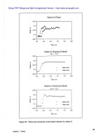
The second case is a comparison to a flume data set reported in Bell, Elliot,
and Ghaudhry (1992) which is analogous to a dam break problem. Here the
shock is in a horseshoe-shaped channel and the comparison is
to
actual flume
data. The comparisons are made to the water surface heights and timing of the
shock passage.

The final case is a steady-state comparison to flume data reported in Ippen
and Dawson (1951). Here a lateral transition under supercritical flow condi-
tions generates a field of oblique jumps. The model comparison is made to
these conditions, which is a more general 2-D domain than previous tests.
Chapter
3
Testing
Simpo PDF Merge and Split Unregistered Version -
Case
1
:
Analytic
Shock
Speed
The shock speed for the shallow-water equations given simple
1-B
geometry can be determined analytically. These are the Rankine-Nugoniot
relations shown in Equations
5
and 9. This provides a direct comparison with
the model shock speed without relying upon hydraulic flume data, for which
discrepancy will be due to the hydrostatic assumption made in the
shallow-
water equations. Instead we have a direct way of evaluating the numerical
scheme alone.
As
spatial and temporal resolution increase, the numerical
shock speed should converge to the analytic speed.
The test consists of setting
a

supercritical flow in a long channel, closing the downstream end, and
calculating the speed of the jump that forms and propagates upstream.
The
initial conditions for this test case are shown in Table
1.
The test conditions
are shown in Table
2.
The term
at
indicates the
method applied
to
the temporal derivative,
1.0
is first-order backward, and
1.5
is
second-order backward. The subscript
s
indicates the value
in
the shock
vicinity. The
a
and
a,
are the weighting of the Petrov-Galerkin contribution
throughout the domain and in the shock vicinity, respectively. With
Manning's n and viscosity of

0.0
there is no dissipation in the shallow-water
equations.
Figures
6-8
and 9-11 show the center-line profile over time of these tests
for
at
=
1.0
and for
AX
=
0.4
and
0.8
m, respectively. These plots represent
the center-line depth profile over time in a perspective view. The vertical axis
is the flow depth, the horizontal axis is time, and the axis that appears to be
into the page is the distance along the channel. From this one can see that as
Chapter
3
Testing
Simpo PDF Merge and Split Unregistered Version -
Figure
6.
Time-history of center-line water surface elevation profiles;
9
=
1.0,

Ax
=
0.4
m,
At
=
0.4
sec
Figure
7.
Time-history of center-line water surface elevation profiles;
9
=
1
.O,
Ax
=
0.4
m,
At
=
0.8
sec
Chapter
3
Testing
Simpo PDF Merge and Split Unregistered Version -
Figure
8.
Time-history of center-line water surface elevation profiles;

9
=
1.0,
Ax
=
0.4
m,
At
=
1.6
sec
Figure
9.
Time-history
of
center-line water surface elevation profiles;
at
=
1
.O,
Ax
=
0.8
m,
At
=
0.8
sec
Chapter
3

Testing
Simpo PDF Merge and Split Unregistered Version -
Figure 10. Time-history of center-line water surface elevation profiles;
at
=
1
.O,
Ax
=
0.8
m,
At
=
1.6 sec
Figure 11. Time-history of center-line water surface elevation profiles;
o+
=
1
.O,
Ax
=
0.8
m, At
=
3.2
sec
Chapter
3
Testing
Simpo PDF Merge and Split Unregistered Version -