CHL - A Finite Element Scheme for Shock Capturing_5 potx

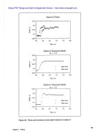
Station
8,
Flume
Tie,
sec
Station
8,
Numerical Model
Tie, sec
Station
8,
Numerical Model
Tie, sec
Figure
26.
Flume and numerical model depth histories for station
8
Chapter
3
Testing
Simpo PDF Merge and Split Unregistered Version -
With this in mind, stations 4 and 8 match fairly closely between flume and
numerical model. Station 4 in the flume would still have a greater difference
between outer and inner wave than that predicted by the model. The differ-
ence might be a manifestation of a three-dimensional effect that the model
cannot mimic. The overall timing and height comparisons are good.
Figure
27
shows the spatial profile of the outer wall water surface elevation
of the numerical model versus distance downstream from the dam. These
distance measurements are in terms of the center-line distance. The two condi-

tions are for
cq
of 1.0 and
1.5,
i.e., first- and second-order temporal derivative.
Channel Center Line Distance,
rn
Figure
27.
Dam break case water surface elevations, comparison of
temporal representation, for time of
3.5
sec
The nodes are delineated by the symbols along the lines. The overshoot of
the second-order scheme and the damping of the first-order is obvious. Again,
it is probable that the overshoot is a numerical artifact even though this is
much like what the flume would show.
Case
3:
2-D
Lateral Transition
This is the most geometrically general case that we test. The numerical
model is compared to flume results. The flume data was reported in Ippen and
Dawson (1951). The tests were conducted for an approach Froude number of
4,
upstream depth of 0.1 ft, (0.03048 m) and a total discharge of 1.44 f&sec
(0.0408 m3/sec). The channel contracts from
2
ft (0.60% m)
to

1
ft
Chapter
3
Testing
Simpo PDF Merge and Split Unregistered Version -
(0.3048 m) wide in a length of 4.78 ft (1.457 m), i.e., an angle of 6 deg on
each side.
The model resolution was increased until we were confident that the results
no longer changed with greater resolution. The numerical model was set up
with 10 evenly spaced elements laterally across the channel and 24 over the
length of the transition. The model limits were extended some 40 ft
(12.192 m).
The total number of nodes was 1661 with 1500 elements.
As
in
the flume test the numerical model was set up to provide a uniform depth of
0.1 ft (0.03048 m) approaching the transition. The bed slope chosen was
0.05664. The other parameters are shown in Table 4.
Since the model was run to steady-state,
at
of 1.0 is appropriate (time
accuracy is irrelevant here).
The results from the numerical model run and the flume results are shown
in
Figure 28. The oblique shock forms along the sidewalls of the transition
and impinges on the point in which the converging channel goes back to paral-
lel walls. This, by the way, is the manner in which one would want to design
a lateral transition. The positive wave from the beginning of the converging
walls will tend to cancel the negative wave originating at the point where the

walls change back to parallel. The heights of the water surface are indicated
by the contours in both model and flume.
The maximum and minimum
heights compare fairly well.
The shape is good as well. Generally the wave
from the shallow-water equation will be swept downstream less than that from
the flume results since the shallow-water equations will transport all wave-
lengths at the speed of a long wave. Shorter waves will travel more slowly
than the shallow-water equations predict. The comparison is good, and the
model demonstrates that the shock capturing technique functions well in a
general 2-D setting.
Chapter
3
Testing
Simpo PDF Merge and Split Unregistered Version -
0.5 0 0.5 1.0
1.5
2.0 2.5 3.0 3.5 4.0 4.5 5.0 5.5 6.0 6.5 7.0
DISTANCE FROM CONTRACTION,
FT
0.5 0 0.5 1.0 1.5 2.0 2.5 3.0 3.5 4.0 4.5 5.0 5.5 6.0
6.5
7.0
DISTANCE FROM CONTRACTION,
FT
Figure
28.
Comparison of flume and numerical model water surface elevations for the super-
critical transition case, straight-wall contraction
F

=
4.0.
To convert feet to
meters, multiply by
0.3048
Chapter
3
Testing
Simpo PDF Merge and Split Unregistered Version -
Discussion
Now let's study the behavior of the 1-D linearized shallow-water equation
analytically and numerically. This could lead
to
a conceptual appreciation of
the behavior we have observed in the testing section of the report. We shall
follow a Fourier analysis of the wave components; for examples, see
Leendertse (1967) or Froehlich (1985). First let's consider the nondimension-
alized shallow-water equations
where, the subscript
*
indicates nondimensional quantities and
o
as a subscript
indicates a constant, and
These equations can be diagonalized by defining a new variable
such that
P:A~P,
=
A,
where

Chapter
3
Testing
Simpo PDF Merge and Split Unregistered Version -
A, is the diagonal matrix of eigenvalues and Po and
P-:
are composed of the
eigenvectors (and are arbitrary). With the substitution of Equation
55
into
54
and multiplication by
P-:
we retrieve the diagonalized shallow-water equations
in
terms of the Riemann Invariants
Now if we consider solutions in terms of
A
where
T
is a constant and
K
is the wave number, we arrive at the solution
where
o
=
m,
the wave frequency
y
=

-io
With this solution we shall now compare the behavior of the model to that of
the analytic solution.
The test function for Equation
54
in
HIVEL2D
would be
Now, since
T
is a linear combination of the variables
h*
and P, we can con-
vert this to the diagonal system as well,
so
that the equivalent test function is
Applying this test function to the discretized differential equation and
substituting
and
Chapter
3
Testing
Simpo PDF Merge and Split Unregistered Version -
where the superscript
n
indicates the time-step and the subscript
j
is the spatial
node location.
We now present the results of this analysis for

a
=
112 and for the temporal
derivative parameter
at
of 1.0 and
1.5.
We shall compare the relative ampli-
tude and relative speed for a single time-step. The parameter for relative speed
is given by
relative
speed
=
tan
where
N
=
elements per wavelength
AAt,
C
=
Courant number
r
-
Ax*
h
=
wave speed, either hl or h2
For
at

=
1,
which is first-order backward difference in time, the relative
amplitude is shown in Figure 29 and the relative wave speed is shown in Fig-
ure 30. This is plotted versus the number of elements per wavelength
N
and
the Courant number
C.
Also
remember that these comparisons apply for either
characteristic
(Al or h2), even for subcritical conditions in which h2 is
negative. In these figures the Courant number varies from
0.5
to 2.0 and the
elements per wavelength from
2
to 10.
The amplitude portrait shows substantial damping for larger
C
and for the
shorter wavelengths (or alternatively the poorer resolution). The large damp-
ing at a wavelength of
2Ax
is important, as this is the mechanism that provides
the energy dissipation to capture shocks. Now consider the phase portrait, or
in this case the relative speed portrait. Over the conditions shown, the numeri-
cal speed is less than
the

analytic speed throughout. For larger
C
the relative
speed is somewhat lower (worse). For
N
=
2 the speed is
0,
so that undamped
oscillation could remain at steady state.
Chapter
3
Testing
Simpo PDF Merge and Split Unregistered Version -
Figure
29.
Relative amplitude versus
C
and resolution for
at
=
1.0 and
a
=
0.5
Figure 30. Relative speed versus
C
and resolution for
at
=

1.0 and
a
=
0.5
Chapter
3
Testing
Simpo PDF Merge and Split Unregistered Version -
In comparison to the results we have shown in Figures 6-11 for Case
1,
analytic shock case, we must remember that C, is the Courant number based
on shock speed, whereas
C
is based on the perturbation wave speed. If we
consider a wave moving upstream just behind the shock, since short wave-
lengths move
t~o slowly, the disturbance of the shock produces waves of these
length which fall behind the shock rather than remaining within.
As
the time-
step is reduced (C, gets smaller) the relative speed is better for the moderate
wavelengths and so the
shock front becomes sharper.
At a point near the shock front we note that generally we get a sharp front
with no undershoot until we reach the smallest time-step. Again if we are
within the shock at a depth where there is an upstream propagating wave
(subcritical), is there a Courant number C that has a relative speed greater than
analytic. This would be the only way in which an undershoot could appear.
Figure
31

extends the relative wave speed portrait below
C
=
0.5. From this
figure it is apparent for small values of C that the numerical wave speed is
greater than analytic so that it is possible to develop an undershoot in front of
the jump.
For
at
=
1.5 we have a second-order temporal derivative which has relative
amplitude and relative speed portraits shown in Figures 32 and 33, respec-
tively.
The degree of damping is much less than for the first-order case. The
relative speed is better but not so dramatic as the improvement in amplitude.
An
interesting point is that the relative speed for
N
=
2
is nonzero for lower C
values. This implies that a spurious mode should not reside in the grid at
steady state. In Figure
34,
we show the relative speed portrait extended below
C values of 0.5.
As
with
q
=

1,
for very low C the numerical relative speed
is greater than the analytic. Therefore, we would expect to have an undershoot
for small time-steps. It should become more pronounced and longer as the
time-step is reduced further. Since we generally have
a
relative speed lower
than analytic, we expect an overshoot behind the jump which becomes longer
as the time-step is increased. Referring to Figures 14-19 of case 1, this is
precisely what we note. Also, for smaller time-steps there is some undershoot
as well. These same features are notable in the second test case, the dam
break test case.
For the sake of completeness the relative amplitude and speed portraits are
included for
a
=
0 and 0.25 at
at
of 1.0 and 1.5 in Figures 35-42. The condi-
tion
a
=
0 is, in fact, the Galerkin case since the Petrov-Galerkin contribution
is included through
a.
The Galerkin approach is shown to contain a steady-
state spurious mode due to the speed of zero for
N
=
2. Furthermore, this

mode is undamped. The case of
a
=
0.25 shows that the relative speed
portraits change very little from
a
=
0.5 but the amplitude damping is
improved.
The obvious conclusions that can be drawn from this discussion is that for
an unsteady run either use
at
=
1.5 or take smaller time-steps with
at
=
1.0.
An
improvement in spatial resolution dramatically improves the solution.
Chapter
3
Testing
Simpo PDF Merge and Split Unregistered Version -
Relative Speed
0
-
Elements per Wavelength
10
Figure
31.

Relative speed versus
C
and resolution for
at
=
1.0 and
a
=
0.5, for
small values of
C
Relative Amplitude
0.
Elements per Wavelength
Figure
32.
Relative amplitude versus
C
and resolution for
at
=
1.5 and
a
=
0.5
Chapter
3
Testing
Simpo PDF Merge and Split Unregistered Version -
Relative Speed

0
.
Elements per Wavelength
Figure
33.
Relative speed versus
C
and resolution for
at
=
1.5 and
a
=
0.5
Relative Speed
0
.
Elements per Wavelength
10
Figure
34.
Relative speed versus
C
and resolution for
at
=
1.5 and
a
=
0.5, for

small values of
C
Chapter
3
Testing
Simpo PDF Merge and Split Unregistered Version -