An Introduction to Financial Option Valuation: Mathematics, Stochastics and Computation_7 pdf

11.5 Change of variables 109
0
E
0
T
S
t
P
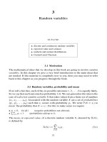
Fig. 11.4. European put: Black–Scholes surface with asset path superimposed.
E
0
T
S
t
delta
Fig. 11.5. Black–Scholes surface for delta with three asset paths superimposed.
110 More on the Black–Scholes formulas
We will introduce three new dimensionless quantities. First is the moneyness
ratio
m := log
Se
r(T −t)
E
.
To interpret m,weneed to generalize (6.11) into the formula Se
µ(T −t)
for the ex-
pected value of the asset at expiry, given asset price S at time t,Nowwemake the
assumption that the asset growth rate equals the interest rate, µ = r. This assump-
tion will be examined in detail in Chapter 12; for now, we simply note that it leads
to the following conclusions.

If m > 0, then the expected asset value at expiry is greater than the strike price. In a ‘risk-
neutral expectation at expiry’ sense, a call option is in-the-money and a put option
is out-of-the-money.
If m = 0, then, in the same sense, call and put options are at-the-money.
If m < 0, then, in the same sense, a call option is out-of-the-money and a put option is
in-the-money.
Second, we have the scaled volatility
τ := σ
√
T − t.
Here, the volatility is combined with the square root of the time to expiry. This
is natural, since, for example, volatility appears in the form σ
2
(t
i+1
−t
i
) in the
underlying asset model (6.9). The third step is to scale the option values by the
asset price, by letting
c :=
C
S
, for a call option,
and
p :=
P
S
, for a put option.
In these new variables, d

1
and d
2
in (8.20) and (8.21) simplify to
d
1
=
m
τ
+
τ
2
and d
2
=
m
τ
−
τ
2
, (11.1)
and, from (8.19) and (8.24), the re-scaled call and put values become
c(m,τ)= N(d
1
) − e
−m
N(d
2
) and p(m,τ)= e
−m

N(−d
2
) − N(−d
1
),
(11.2)
see Exercise 11.3.
11.7 Program of Chapter 11 and walkthrough 111
11.6 Notes and references
Colour versions of Figures 11.3, 11.4 and 11.5 can be downloaded from this book’s
website, mentioned in the preface.
EXERCISES
11.1.  Consider the following ‘explanation’ of why the Black–Scholes Euro-
pean call option value curve C(S, t) lies above the payoff hockey stick
max(S(t) − E, 0), for t < T.
Since E(S(t)) = S
0
e
µt
, the asset price generically drifts upwards. Hence, on aver-
age, the asset price will increase between time t and expiry, so the time t value is
greater than max(S(t) − E, 0).
Is this argument valid?
11.2.  Show how Exercise 10.7 provides a counterexample to the following
statement:
As t goes from 0 to T, the Black–Scholes European put option value always ap-
proaches the payoff hockey-stick function from below.
11.3.  Verify (11.1) and (11.2).
11.4. In the case where the volatility, σ ,iszero in the asset model (6.9), the
final asset price is the nonrandom quantity S

0
e
µT
. The payoff from a Eu-
ropean option is then guaranteed to be max(S
0
e
µT
− E, 0).Itmay thus be
argued that the time-zero option value must be e
−rT
max(S
0
e
µT
− E, 0).
However, this value clearly depends upon µ, whilst the Black–Scholes for-
mula does not. (In fact, looking ahead to (14.2), the Black–Scholes value is
e
−rT
max(S
0
e
rT
− E, 0).) Can you resolve this apparent contradiction?
11.5.  Show that ‘Call(−σ) =−Put(σ )’, that is, replacing σ in (8.19) by −σ
is equivalent to evaluating −P(S, t) in (8.24). This relation is sometimes
called put–call supersymmetry.
11.7 Program of Chapter 11 and walkthrough
The program ch11 plots the Black–Scholes surface above the (S, t)-plane for a European call, in

the style of Figure 11.3. It is listed in Figure 11.6. We initialize E,r,sigma and T, and set up the
array Svals of 50 equally spaced asset prices between 0 and 3 and the array tvals of 50 equally
spaced time points between 0 and T. The nested for loops then work through Svals and tvals,
using ch08 to evaluate the Black–Scholes formula. The European call value is stored in the two-
dimensional array Call.Wethen use meshgrid to set up two-dimensional arrays Smat and tmat
that are appropriate for use with the three-dimensional plotting function mesh.
112 More on the Black–Scholes formulas
%CH11 Program for Chapter 11
%
% Draws Black-Scholes surface for European call
clf
%%%%%%%% Problem parameters %%%%%%%%%
E=1; r=0.05; sigma = 0.2; T = 1; L =50;
%%%%%%%%%%%%%%%%%%%%%%%%%%%%
Svals = linspace(0,3,L);
tvals = linspace(0,T,L);
C=zeros(L,L);
for i = 1:L
S=Svals(i);
for j = 1:L
t=tvals(j);
[Call,Calldelta,Put,Putdelta] = ch08(S,E,r,sigma,T-t);
C(i,j) = Call;
end
end
[Smat,tmat] = meshgrid(Svals,tvals);
mesh(Smat,tmat,C’)
ylabel(’S’), xlabel(’t’), zlabel(’C(S,t)’)
Fig. 11.6. Program of Chapter 11: ch11.m.
PROGRAMMING EXERCISES

P11.1. Edit ch11.m so that it applies to a European put option, as in Figure 11.4.
P11.2. Edit
ch11.m so that it applies to the delta of a European call option, as
in Figure 11.5, and investigate the use of
surf, surfc and waterfall instead of
mesh.
Quotes
The Black–Scholes formula is still around,
even though it depends on at least 10 unrealistic assumptions.
Making the assumptions more realistic
hasn’t produced a formula that works better across a wide range of circumstances.
FISCHER BLACK (Black, 1989)
We know this doesn’t work by rote.
But this is the best model we have.
You look at the old-timers who went with their gut.
You had this model, you had these numbers,
11.7 Program of Chapter 11 and walkthrough 113
and in the end you thought they were a lot more powerful than a guy’s gut.
ROBERT STAVIS, former member of the Arbitrage group at Salomon Brothers, source
(Lowenstein, 2001)
A first-rate theory predicts,
a second-rate theory forbids
and a third-rate theory explains after the event.
ALEXANDER KITAIGORODSKI, 1975,
source www.byrneweb.com/sunburn/quotes. html

12
Risk neutrality
OUTLINE
• option value as expected payoff

• risk neutrality
12.1 Motivation
In the days before the Black–Scholes formula, it was often argued that a reasonable
waytovalue an option is to take the expected payoff.Inthis chapter we show how
the expected payoff idea fits in with the Black–Scholes methodology. This leads us
to the concept of risk neutrality, which will play a fundamental role in Chapters 15,
16 and beyond, when we discuss computational algorithms.
12.2 Expected payoff
To cover European call and put options in a single notation, we let (x) denote the
payoff function, so (x) = max(x − E, 0) for a call and (x) = max(E − x, 0)
for a put. The treatment here easily generalizes to other European-style options,
that is, options whose payoff may be expressed as a function of the asset price at
expiry.
Under our model (6.8), the final asset price, S(T ),isarandom variable of the
form S(T) = S
0
e
(µ−σ
2
/2)T +σ
√
TZ
, where Z ∼ N(0, 1).Sothe payoff, (S(T )),
is also a known random variable. Why don’t we simply take the time-zero option
value to be the average payoff, suitably discounted for interest? This gives a value
e
−rT
E((S(T ))). (12.1)
Using (3.8) and the density function (6.10), this may be written
e

−rT

∞
0
(x)
xσ
√
2π
√
T
exp



−

log x − log S
0
− (µ −
1
2
σ
2
)T

2
2σ
2
T




dx. (12.2)
115
116 Risk neutrality
More generally, we could regard the option value at asset price S and time t as the,
suitably discounted, expectation of the payoff. Letting W(S, t) denote this value,
we have
W(S, t) = e
−r(T−t)
E
(
(S(T )), given asset price S at time t
)
, (12.3)
which may be written more explicitly as
W(S, t) = e
−r(T−t)

∞
0
(x)
xσ
√
2π
√
T − t
exp




−

log x − log S − (µ −
1
2
σ
2
)(T − t)

2
2σ
2
(T − t)



dx. (12.4)
The values (12.2) and (12.4) are certainly relevant to an individual who is in the
habit of writing or holding naked options. However, in comparison with the Black–
Scholes approach to finding a fair option value, there are a number of related points
to make.
(i) Formulas (12.2) and (12.4) were derived without any reference to the idea of hedging
to eliminate risk.
(ii) Formulas (12.2) and (12.4) were derived without any reference to the no arbitrage
principle.
(iii) Unlike the Black–Scholes PDE (8.15), the formulas (12.2) and (12.4) depend on the
parameter µ.
Now the Black–Scholes theory tells us that there is only one fair value, and
this must be the figure quoted in the market. If the market placed the option

lower/ higher, arbitrageurs would swoop en masse, buying/selling the option, delta
hedging until expiry, and hence guaranteeing a riskless profit. The forces of supply
and demand therefore constrain the option to the Black–Scholes level. It follows
from point (iii) that the expected payoff approach cannot be used to get a fair value.
On the face of it, expected payoff seems to have no place in option valuation
theory. However, by a remarkable twist, it is possible to rehabilitate the idea.
12.3 Risk neutrality
Figure 12.1 confirms that the time-zero discounted expected payoff (12.2) is indeed
a function of µ. The solid line plots (12.2) as µ varies from 0 to 0.1 for a European
call with S
0
= 10, E = 9, r = 0.05, σ = 0.2andT = 3. As we would guess, the
expected payoff increases with the growth rate, µ. Superimposed on the picture as
a dashed line is the Black–Scholes option value, 2.66.
12.3 Risk neutrality 117
0 0.01 0.02 0.03 0.04 0.05 0.06 0.07 0.08 0.09 0.1
1.5
2
2.5
3
3.5
4
4.5
µ
Discounted expected payoff
Black–Scholes value
Fig. 12.1. Time-zero discounted expected payoff (12.2) for a European call.
Black–Scholes value superimposed as a dashed line.
Keen-eyed observers will note that the solid curve in Figure 12.1 appears to
pass through the Black–Scholes level at the value µ = r = 0.05; that is, when the

growth rate parameter matches the interest rate. This turns out to be no coinci-
dence. Exercise 12.1 asks you to verify the general result that
W(S, t) in (12.4) satisfies the Black–Scholes PDE (8.15) when µ = r.
Now we check the final time and boundary conditions. Taking t = T in (12.3),
we note that if S(T ) is given, and thus nonrandom, then
E((S(T ))) = (S(T)),
giving
W(S, T) = (S(T)).
Hence the conditions (8.16) for a call and (8.25) for a put are satisfied. Similarly,
if S = 0atany time then we know from (6.9) that S(T) = 0, and hence in (12.3)
W(0, t) = e
−r(T−t)
(0).
This matches (8.17) and (8.26) for the call and put, respectively. Finally, we note
that the arguments given to justify (8.18) and (8.27) are equally valid for (12.3).
Overall, since W(S, t) with µ = r satisfies the same PDE and the same final
time/ boundary conditions, the uniqueness of the solution tells us that
118 Risk neutrality
W(S, t) in (12.4) reproduces the Black–Scholes option value when µ = r.
We could re-write this conclusion as follows.
No matter what parameters µ and σ in the asset model (6.9) we believe to be correct, we
can obtain the Black–Scholes option value by pretending that the drift, µ,isequal to the
interest rate, r, and taking the discounted expected payoff.
In setting µ = r we are making what is known as a risk neutrality assumption.
We will see in Chapters 15 and 16 that the risk-neutral expectation framework
allows us to develop computational methods for approximating options where an-
alytical formulas are not available.
12.4 Notes and references
It is perfectly standard, but not particularly enlightening, to give the name risk
neutrality to the condition µ = r. The phrase borrows from the concept of a risk-

neutral investor;anunlikely person who regards
• an investment with guaranteed rate of return r, and
• a risky investment with expected rate of return r
as equally attractive. In the case where all assets satisfy the lognormal model (6.9)
with the same growth parameter µ – the so-called risk-neutral world –wesee from
(6.11) that a risk-neutral investor would have no preferences between investing in
a bank and in any asset.
In the risk-neutral world, (6.11) shows that
E(S(t)) = S
0
e
rt
,sothe expected
discounted asset price is
E(e
−rt
S(t)) = S
0
.Inother words, the expected dis-
counted asset price does not change with time; it remains at its time-zero level. A
process like this, whose expected future value is given by its current value, is called
a martingale.Byusing martingale theory it is possible to convert the simple obser-
vation in Exercise 12.1 into a rigorous and powerful theory for option valuation.
In particular, this is an alternative way to derive the Black–Scholes formulas. The
texts (Duffie, 2001; Karatzas and Shreve, 1998; Nielsen, 1999) cover this material
in depth, while perhaps the most accessible introduction is (Baxter and Rennie,
1996). Chapter 6 of (Kritzman, 2000) also gives a very readable, example-driven
coverage of risk neutrality.
In Chapter 16 we introduce the binomial method as a computational technique
for option valuation. It is also possible to use the binomial framework as an

analytical tool with which the Black–Scholes formulas can be derived without
recourse to PDEs. The concept of risk neutrality arises quite naturally in this
setting. Exercise 12.5 provides a cut-down version of the idea. The text (Baxter
12.4 Notes and references 119
and Rennie, 1996) and the on-line lecture notes of Professor Robert Kohn at
www.math.nyu.edu/faculty/kohn/ are good places to learn more.
EXERCISES
12.1. Using a large sheet of paper and a pen with plenty of ink, show that
for µ = r the quantity W(S, t) in (12.4) satisfies the Black–Scholes PDE
(8.15). (You may differentiate inside the integral sign without worrying
about whether this is justified.)
12.2.  Consider a European-style option with payoff at expiry given by
(S(T )) = S(T). Explain why the time-zero value of this option must be
S
0
.Byusing (6.11), show that asking for the discounted expected payoff
(12.1) to match this value leads immediately to the risk neutrality condition
µ = r.
12.3.  Given initial asset price S
0
at time t = 0, show that, in a risk-neutral
world, the factor N(d
2
) in the Black–Scholes formula (8.19) represents the
probability that a European call option will be exercised.
12.4. Show that the value W(S, t) in (12.4) can be computed from the fol-
lowing recipe.
(i) Compute the Black–Scholes option value at (S, t) with the interest rate set
to r = µ.
(ii) Scale this quantity by e

(µ−r)(T−t)
.
(This recipe was used to create Figure 12.1.)
12.5. Consider the following, simplified scenario for valuing a European-
style option.
• The time-zero asset price is S
0
.
• At expiry, the asset price may take only two possible values
S(T) = S
up
> S
0
, with probability p,
S(T) = S
down
< S
0
, with probability 1 − p.
Let  denote the payoff function, and let 
up
:= (S
up
) and 
down
:=
(S
down
) denote the two possible payoffs at expiry. Take a portfolio at time
t = 0 consisting of A units of asset and an amount C of cash. Asking for

this portfolio to replicate the option (i.e. to have payoff 
up
when S(T) =
S
up
and 
down
when S(T ) = S
down
) leads to a pair of linear equations for
A and C. Find and solve these to obtain
A =

up
− 
down
S
up
− S
down
, (12.5)
120 Risk neutrality
C = e
−rT


down
−



up
− 
down
S
up
− S
down

S
down

. (12.6)
Then use the no arbitrage principle to deduce that a fair time-zero value for
the option is
S
0


up
− 
down
S
up
− S
down

+ e
−rT

S

up

down
− S
down

up
S
up
− S
down

. (12.7)
Now, let
q :=
S
0
e
rT
− S
down
S
up
− S
down
.
Use the no arbitrage principle to argue that 0 < q < 1 must hold. Show
that the value in (12.7) may also be interpreted as the discounted expected
payoff of an asset taking the values
S(T) = S

up
> S
0
, with probability q,
S(T) = S
down
< S
0
, with probability 1 − q.
Can you see any features from this simplified scenario that carry through
to the Black–Scholes version?
12.6. In Section 10.3 we gave a financial interpretation of the inequality ρ>
0. Use the risk neutrality viewpoint to give an alternative interpretation.
12.5 Program of Chapter 12 and walkthrough
The program ch12,listed in Figure 12.2, illustrates risk neutrality in the manner of Figure 12.1. We
fix S,E,r,sigma and T and an array of 200 values for mu.Afor loop is then used to compute an
array epayoff which stores the discounted time-zero Black–Scholes value when r is set to each mu
value; see Exercise 12.4. This is done via the ch08 function from Chapter 8. After executing this
loop, we use ch08 to obtain the true Black–Scholes value, C.Wethen plot the (muvals,epayoff)
curve and superimpose a dashed line at height C.
PROGRAMMING EXERCISES
P12.1. Confirm experimentally the result mentioned in Exercise 12.3. Do this by
generating a large number of expiry-time asset prices, and counting the proportion
that are in-the-money.
P12.2. Investigate the use of
quad and quadl for evaluating integrals of the form
(12.4).
12.5 Program of Chapter 12 and walkthrough 121
%CH12 Program for Chapter 12
%

% Compute expected payoff for European call
% Illustrates risk neutrality
clf
%%%%% Problem parameters %%%%%%
S=5; E=7; r=0.08; sigma = 0.3; T = 1;
M=200; muvals = linspace(0,0.16,M);
%%%%%%%%%%%%%%%%%%%%%%%
epayoff = zeros(M,1);
for k = 1:M
mu = muvals(k);
% work out time-zero Black-Scholes value withr=mu
[C, Cdelta, P, Pdelta] = ch08(S,E,mu,sigma,T);
epayoff(k) = exp((mu-r)*T)*C;
end
% true Black–Scholes value
[C, Cdelta, P, Pdelta] = ch08(S,E,r,sigma,T);
plot(muvals,epayoff,’r-’);
hold on, grid on
plot([muvals(1),muvals(end)],[C,C],’b-’);
xlabel(’\mu’), legend(’Expected payoff’,’Black-Scholes’)
Fig. 12.2. Program of Chapter 12: ch12.m.
Quotes
risk-neutrality is far from easy to grasp intuitively,
which is perhaps the source of the confusion above.
The key steps in the derivation of the Black–Scholes equation,
namely no arbitrage and that risk-free portfolios can earn the risk-free rate,
are intuitively clear.
PAUL WILMOTT, SAM HOWISON AND JEFF DEWYNNE (Wilmott et al., 1995)
Risk neutral valuation, which was developed by John Cox and Stephen Ross,
has the dual virtues that it can be applied to practically any option valuation problem

and it is marvelously intuitive.
MARK P. KRITZMAN (Kritzman, 2000)
To put it simply,
if there is an arbitrage price, any other price is too dangerous to quote.
MARTIN BAXTER AND ANDREW RENNIE (Baxter and Rennie, 1996)

13
Solving a nonlinear equation
OUTLINE
• general problem
• bisection method
• Newton’s method
13.1 Motivation
In the next chapter, where we look at computing the implied volatility, we will
need an algorithm for solving a nonlinear equation. This chapter introduces two
such algorithms.
13.2 General problem
The task that we consider in this chapter is
given a function F : R → R, find an x

∈ R such that F(x

) = 0.
In general, of course, we cannot find an x

analytically, and must therefore con-
tent ourselves with an approximation via a computational method. It is also worth
keeping in mind that, depending on the nature of F, there may be no suitable x

,

exactly one x

or many x

values.
13.3 Bisection
The bisection method is based on the observation that if a continuous function
changes sign then it must pass through zero; that is,
for continuous F,ifx
a
< x
b
with F(x
a
)F(x
b
)<0,
then F(x

) = 0 for some x
a
< x

< x
b
.
Having found x
a
and x
b

with F(x
a
)F(x
b
)<0, we could evaluate F at the mid-
point x
mid
:= (x
a
+ x
b
)/2. The sign of F(x
mid
) must then match either F(x
a
) or
123
124 Solving a nonlinear equation
F(x
b
).This means that one of the intervals [x
a
, x
mid
]or[x
mid
, x
b
] must contain
an x


.Byrepeating this process, we can construct an arbitrarily small interval in
which an x

must lie – hence we can find an x

to any level of accuracy.
We may thus spell out the bisection method as follows.
Step 1: Find x
a
and x
b
with x
a
< x
b
such that F(x
a
)F(x
b
) ≤ 0.
Step 2: Set x
mid
:= (x
a
+ x
b
)/2 and evaluate F(x
mid
).

Step 3: If F(x
a
)F(x
mid
)<0 then reset x
b
= x
mid
.
Otherwise reset x
a
= x
mid
.
Step 4: If x
b
− x
a
<εthen stop. Use
1
2
(x
a
+ x
b
) as the approximation to x

.
Otherwise return to Step 2.
Note that we must choose a value ε>0 for our stopping criterion x

b
− x
a
<ε.
It is easy to see that the value (x
a
+ x
b
)/2ontermination is no more than a distance
ε/2 from a solution x

. Hence, ε controls the accuracy of the process.
There is no foolproof procedure for finding suitable x
a
and x
b
in Step 1. Without
specific knowledge of the function F we must resort to trial and error.
Because the bisection method halves the length of the interval [x
a
, x
b
]oneach
iteration, we may bound the error at the kth iteration by L/2
k+1
, where L is the
length of the original interval, x
b
− x
a

. This is referred to as a linear convergence
bound because the error bound decreases by a linear factor, in this case
1
2
,oneach
iteration. We consider next a faster method.
13.4 Newton
Newton’s method (also called the Newton–Raphson method) can be derived in
a number of ways. We will use a Taylor series approach. Suppose we wish to
compute a sequence x
0
, x
1
, x
2
, that converges to a solution x

.Wemay expand
F(x
n
+ δ) for small δ by
F(x
n
+ δ) = F(x
n
) + δ F

(x
n
) + O(δ

2
). (13.1)
Ignoring the O(δ
2
) term and setting F(x
n
) + δ F

(x
n
) = 0givesδ =
−F(x
n
)/F

(x
n
).Itfollows that if x
n
is close to a solution x

then
x
n+1
= x
n
−
F(x
n
)

F

(x
n
)
(13.2)
should be even closer. Given a starting value, x
0
, the iteration (13.2) defines New-
ton’s method.
Since we discarded an O(δ
2
) term in (13.1), we may expect that the error
13.4 Newton 125
x
n
− x

squares as n increases to n +1; that is, if x
n
− x

= O(δ) then x
n+1
−
x

= O(δ
2
).Tosee this more clearly, note that, using F(x


) = 0 and assuming
F

(x
n
) = 0in(13.2), a Taylor series gives
x
n+1
− x

= x
n
− x

−

F(x
n
) − F(x

)
F

(x
n
)

= x
n

− x

−
(x
n
− x

)F

(x
n
) + O

(x
n
− x

)
2

F

(x
n
)
= O

(x
n
− x


)
2

. (13.3)
This type of analysis can be formalized to give the following result.
Theorem 1 Suppose F has a continuous second derivative, and suppose x

∈
R satisfies F(x

) = 0 and F

(x

) = 0. Then there exists a δ>0 such that for
|x
0
− x

| <δthe sequence given by (13.2) is well defined for all n > 0,
lim
n→∞
|x
n
− x

|=0
and there exists a constant C such that
|x

n+1
− x

|≤C|x
n
− x

|
2
. (13.4)

The bound (13.4) shows that Newton’s method has quadratic or second or-
der convergence. However, the result requires the starting value x
0
to be chosen
sufficiently close to x

.Inpractice Newton’s method works very well when a
suitable x
0
is found, but may fail to converge otherwise.
Computational example Suppose we wish to find the value of x

such that
P
(
X ≤ x

)
=

2
3
, where X ∼ N(0, 1). Equivalently, we want to solve F(x) = 0,
where F(x) := N(x) −
2
3
with N(x) defined in (3.18). It follows from the defi-
nition of N(x) that F(x) is an increasing function of x with F(0) =
1
2
−
2
3
< 0
and lim
x→∞
F(x) = 1 −
2
3
> 0. Hence, we may immediately conclude that
F(x) = 0 has a unique solution 0 < x

< ∞. This can be confirmed from the
plot of F(x) in Figure 13.1. We may apply the bisection method with x
a
= 0
and with x
b
sufficiently large that F(x
b

)>0. For the choice x
b
= 10 and a tol-
erance of ε = 10
−5
in the stopping criterion, the errors |x
mid
− x

| are shown as
asterisks in the left-hand plot of Figure 13.2. Note that the y-axis is logarithmi-
cally scaled. We see that 20 iterations were taken in the bisection method. The
dashed line corresponding to 10 ×

1
2

k+1
has been added to the plot. The pre-
ceding analysis shows that the error lies below this line. The right-hand plot in
Figure 13.2 shows the corresponding errors for Newton’s method. Here we set
126 Solving a nonlinear equation
− 5 − 4 − 3 − 2 − 1 0 1 2 3 4 5
− 0.8
− 0.6
− 0.4
− 0.2
0
0.2
0.4

0.6
x
F
(
x
)
Fig. 13.1. The function F(x) := N(x) −
2
3
.
0 5 10 15 20
10
− 7
10
− 6
10
− 5
10
− 4
10
− 3
10
− 2
10
−1
10
0
10
1
Bisection

Error
Iteration
1 2 3 4
10
−12
10
−10
10
− 8
10
− 6
10
− 4
10
−2
10
0
Newton
Error
Iteration
Fig. 13.2. Error in the bisection method (left) and Newton’s method (right). A
reference line of slope −1 has been added in the left-hand plot.
13.6 Notes and references 127
x
0
= 1 and stopped when |x
n+1
− x
n
| < 10

−5
.Wesee that only 4 iterations were
required to produce an error of around 10
−12
, and the error roughly squares from
one step to the next. Repeating Newton’s method with x
0
= 2, however, resulted
in a sequence that ‘blew up’ – the numbers became too large for the computer to
store. ♦
13.5 Further practical issues
There are many issues that we have not addressed here. It is possible, for exam-
ple, to design a hybrid algorithm that uses a safe method, like bisection, until
the iterates are close to an x

and then switches to Newton’s method to get the
benefit of rapid convergence. Also, the residual |F(x
n
)| gives a measure of how
close x
n
is to a solution, and this can be incorporated into the stopping criterion.
Furthermore, although we have considered only a single nonlinear equation, it is
possible to generalize Newton’s method to the case of many equations in many
unknowns.
13.6 Notes and references
Most introductory numerical analysis texts have a chapter on solving nonlinear
equations. An excellent and up-to-date specialist treatment that includes MAT-
LAB codes is (Kelley, 1995). The classic advanced text is (Ortega and Rheinboldt,
1970).

If you need to brush up on Taylor series, order notation and, for the next chap-
ter, the Mean Value Theorem, there are many introductory texts to choose from;
(Estep, 2002) is an excellent modern treatment.
EXERCISES
13.1.  Suppose that Step 1 of the bisection method has been completed for a
continuous function F and let L = x
b
− x
a
.Interms of L and ε,howmany
iterations of Steps 2–4 will be taken? Check that your answer is consistent
with the left-hand plot in Figure 13.2.
13.2.  Consider the following approach to computing a sequence of approxima-
tions x
0
, x
1
, x
2
, to x

.Givenx
n
, let x
n+1
be the solution to p
n
(x) = 0,
where p
n

(x) is an approximation to F(x) determined by the three con-
ditions (a) p
n
(x) is linear, (b) p
n
(x
n
) = F(x
n
) and (c) p

n
(x) = F

(x
n
).
Draw a picture to illustrate this construction and then show that x
n+1
is given by (13.2). (Hence, this is an alternative derivation of Newton’s
method.)
128 Solving a nonlinear equation
13.3.  To compute the errors that are shown in Figure 13.2 it was ne-
cessary to obtain the exact solution x

. This was done by setting
xstar = sqrt(2)*erfinv(1/3) where erfinv is MATLAB’s built-in
routine to evaluate the inverse error function described in Exercise 4.3.
Confirm that
xstar is the required solution.

13.4.  Look at Figure 13.1. Using a ruler and pencil, and following the lin-
earization approach in Exercise 13.2, convince yourself that Newton’s
method will converge with the starting value x
0
= 1, but will not converge
with the starting value x
0
= 2.
13.7 Program of Chapter 13 and walkthrough
In ch13, listed in Figure 13.3, we apply Newton’s method to N(x) + e
x
= 2. The line
exact = fzero(inline(‘0.5*(1+erf(x/sqrt(2))) + exp(x)- 2’),1);
%CH13 Program for Chapter 13
%
% Apply Netwon’s method to N(x) + exp(x) = 2.
exact = fzero(inline(’0.5*(1+erf(x/sqrt(2))) + exp(x)- 2’),1);
x0=1;
x=x0;
xdiff = 1;
k=1;
kmax = 100;
tol = 1e-8;
while (xdiff >= tol&k<kmax)
Fval = 0.5*(1+erf(x/sqrt(2))) + exp(x) - 2;
Fprime = exp(-0.5*xˆ2)/sqrt(2*pi) + exp(x);
increment = Fval/Fprime;
x=x-increment;
xnewton(k) = x;
newterr(k) = abs(xnewton(k)-exact);

k=k+1;
xdiff = abs(increment);
end
format short e % non-default for number display
disp(’Newton error’)
disp(newterr’)
format % reset to default for number display
Fig. 13.3. Program of Chapter 13: ch13.m.
13.7 Program of Chapter 13 and walkthrough 129
uses MATLAB’s built-in equation solver fzero to compute an ‘exact’ solution, which we
use for reference. The syntax
while (xdiff >= tol&k<kmax)
.
.
end
sets up a loop that repeats while both xdiff >= tol and k<kmax remain true. In other
words, the loop terminates when either xdiff drops below tol or the maximum number,
kmax,ofiterations has been reached. Inside the loop we implement Newton’s method for
the problem. The error in each iterate is stored in the array newterr.
On exiting the loop, we output the errors. The line format short e sets up a number
display format that is appropriate for this output. At the end of the program we reset the
display to the default with format.
Output from ch13 is
Newton error
1.5465e-01
8.3622e-03
2.4964e-05
2.2279e-10
1.1102e-16
This is consistent with the quadratic convergence discussed in Section 13.4 – the error

roughly squares from one iteration to the next until it reaches a level that the machine
cannot distinguish from zero.
PROGRAMMING EXERCISES
P13.1. Investigate the convergence of the bisection method on the problem solved
by
ch13.
P13.2. Using your answer to programming exercise P12.2, apply bisection to con-
firm that the two curves displayed in Figure 12.1 intersect at µ = r.
Quotes
Chance has put in our way a most singular and whimsical problem,
and its solution is its own reward.
SHERLOCK HOLMES,inThe Adventure of the Blue Carbuncle by Sir Arthur Conan
Doyle
A blunder is an accidental mistake,
as opposed to an approximation error, which is merely a compromise.
ROBERT M. CORLESS (Corless, 2002)