An Introduction to Financial Option Valuation: Mathematics, Stochastics and Computation_13 pot

23.5 FTCS and BTCS 241
x
t
0
T
L
Fig. 23.2. Finite difference grid {jh, ik}
N
x
, N
t
j=0,i=0
. Points are spaced at a distance
of h apart in the x-direction and k apart in the t-direction.
A simple method for the heat equation (23.2) involves approximating the time
derivative ∂/∂t by the scaled forward difference in time, k
−1

t
, and the second
order space derivative ∂
2
/∂x
2
by the scaled second order central difference in
space, h
−2
δ
2
x
. This gives the equation

k
−1

t
U
i
j
− h
−2
δ
2
x
U
i
j
= 0,
which may be expanded as
U
i+1
j
− U
i
j
k
−
U
i
j+1
− 2U
i

j
+ U
i
j−1
h
2
= 0.
A more revealing re-write is
U
i+1
j
= νU
i
j+1
+ (1 − 2ν)U
i
j
+ νU
i
j−1
, (23.7)
where ν := k/h
2
is known as the mesh ratio.
Suppose that all approximate solution values at time level i, {U
i
j
}
N
x

j=0
, are
known. Now note that U
i+1
0
= a((i + 1)k) and U
i+1
N
x
= b((i + 1)k) are given by
the boundary conditions (23.4). Equation (23.7) then gives a formula for comput-
ing all other approximate values at time level i + 1, that is, {U
i+1
j
}
N
x
−1
j=1
. Since we
242 Finite difference methods
Fig. 23.3. Stencil for FTCS. Solid circles indicate the location of values that
must be known in order to obtain the value located at the open circle.
are supplied with the time-zero values, U
0
j
= g( jh) from (23.3), this means that
the complete set of approximations {U
i
j

}
N
x
, N
t
j=0,i=0
can be computed by stepping for-
ward in time. The method defined by (23.7) is known as FTCS, which stands for
forward difference in time, central difference in space. Figure 23.3 illustrates the
stencil for FTCS. Here, the solid circles indicate the location of values U
i
j−1
, U
i
j
and U
i
j+1
that must be known in order to obtain the value U
i+1
j
located at the open
circle.
We may collect all the interior values at time level i into a vector,
U
i
:=









U
i
1
U
i
2
.
.
.
.
.
.
U
i
N
x
−1









∈
R
N
x
−1
. (23.8)
Exercise 23.3 then asks you to confirm that FTCS may be written
U
i+1
= FU
i
+ p
i
, for 0 ≤ i ≤ N
t
− 1, (23.9)
with
U
0
=








g(h)
g(2h)

.
.
.
.
.
.
g((N
x
− 1)h)








∈
R
N
x
−1
,
23.5 FTCS and BTCS 243
where the matrix F has the form
F =













1 − 2νν 0 0
ν 1 − 2νν 0
.
.
.
.
.
.
0
.
.
.
.
.
.
.
.
.
.
.
.
.

.
.
.
.
.
.
.
.
.
.
.
.
.
.
.
.
.
0
.
.
.
.
.
.
.
.
.
.
.
.

1 − 2νν
0 0 ν 1 − 2ν












∈
R
(N
x
−1)×(N
x
−1)
,
and the vector p
i
has the form
p
i
=











νa(ik)
0
.
.
.
.
.
.
0
νb(ik)










∈
R

N
x
−1
.
Here, FU
i
denotes a matrix–vector product.
Computational example Figure 23.4 illustrates a numerical solution produced
by FTCS on the problem of Figure 23.1, with T = 3. We chose N
x
= 14 and
N
t
= 199, so h = π/14 ≈ 0.22 and k = 3/199 ≈ 0.015, giving ν ≈ 0.3. The
numerical solution appears to match the exact solution, shown in Figure 23.1.
Computing the worst-case grid error, max
0≤j ≤N
x
,0≤i≤N
t
|U
i
j
− u( jh, ik)|, pro-
duced 0.0012, which confirms the close agreement. As can be seen from
Figure 23.4, we used a grid where k is much smaller than h –wedivided the x-
axis into only 15 points, compared with 200 points on the t-axis. In Figure 23.5
we show what happens if we try to correct this imbalance. Here, we reduced N
t
to 94, so k ≈ 0.032 and ν ≈ 0.63. We see that the numerical solution has de-

veloped oscillations that render it useless as an approximation to u(x, t).Taking
smaller values of N
t
, that is, larger timesteps k,leads to more dramatic oscilla-
tions. In Section 23.7 we develop some theory that explains this behaviour. We
finish this section by deriving an alternative method that is more computationally
expensive, but does not suffer from the type of instability seen in Figure 23.5. ♦
Replacing the forward difference in time in FTCS by a backward difference
gives
k
−1
∇
t
U
i
j
− h
−2
δ
2
x
U
i
j
= 0,
244 Finite difference methods
0
5
10
15

0
50
100
150
200
0
0.2
0.4
0.6
0.8
1
x
FTCS: ν = 0.3
t
Fig. 23.4. FTCS solution on the heat equation (23.2), (23.3) and (23.4) with
initial and boundary conditions (23.5). Here N
x
= 14 and N
t
= 199, so ν ≈ 0.3.
or, in more detail,
U
i
j
− U
i−1
j
k
−
U

i
j+1
− 2U
i
j
+ U
i
j−1
h
2
= 0.
It is convenient to write this as a process that goes from time level i to i + 1, that
is, to increase the time index by 1, which allows the method to be written
U
i+1
j
= U
i
j
+ ν

U
i+1
j+1
− 2U
i+1
j
+ U
i+1
j−1


. (23.10)
The method defined by (23.10) is known as BTCS, which stands for backward
difference in time, central difference in space. Figure 23.6 illustrates the stencil for
BTCS. Unlike FTCS, with BTCS there is no explicit way to compute {U
i+1
j
}
N
x
−1
j=1
from {U
i
j
}
N
x
−1
j=1
. Using the vector notation (23.8), Exercise 23.4 asks you to show
that the recurrence (23.10) for BTCS may be written
BU
i+1
= U
i
+ q
i
, for 0 ≤ i ≤ N
t

− 1, (23.11)
23.5 FTCS and BTCS 245
0
5
10
15
0
20
40
60
80
100
−1.5
−1
−0.5
0
0.5
1
1.5
x
FTCS: ν = 0.63
t
Fig. 23.5. FTCS solution on the heat equation (23.2), (23.3) and (23.4) with
initial and boundary conditions (23.5). Here N
x
= 14 and N
t
= 94, so ν ≈ 0.63.
where the matrix B has the form
B =













1 + 2ν −ν 0 0
−ν 1 + 2ν −ν 0
.
.
.
.
.
.
0
.
.
.
.
.
.
.
.
.

.
.
.
.
.
.
.
.
.
.
.
.
.
.
.
.
.
.
.
.
.
0
.
.
.
.
.
.
.
.

.
−ν 1 + 2ν −ν
0 0 −ν 1 + 2ν












∈
R
(N
x
−1)×(N
x
−1)
,
(23.12)
and the vector q
i
has the form
q
i
=











νa((i + 1)k)
0
.
.
.
.
.
.
0
νb((i + 1)k)











∈
R
N
x
−1
.
246 Finite difference methods
Fig. 23.6. Stencil for BTCS. Solid circles indicate the location of values that
must be known in order to obtain the value located at the open circle.
The formulation (23.11) reveals that, given U
i
,wemay compute U
i+1
by solv-
ing a system of linear equations. This is a standard problem in numerical analysis,
see Section 23.9 for references.
Computational example Figure 23.7 gives the BTCS numerical solution for
the problem in Figure 23.1, with T = 3. We used N
x
= 14 and N
t
= 9, so
h = π/14 ≈ 0.22 and k = 3/9 ≈ 0.33, giving ν ≈ 6.6. The numerical solution
agrees qualitatively with the exact solution in Figure 23.1, and we found that
the worst-case grid error, max
0≤j ≤N
x
,0≤i≤N
t
|U

i
j
− u( jh, ik)|,was a respectable
0.055. ♦
23.6 Local accuracy
It is intuitively reasonable to judge the accuracy of a finite difference method by
looking at the residual when the exact solution is substituted into the difference for-
mula. For FTCS, letting u
i
j
denote the exact solution u( jh, ik), the local accuracy
is defined to be
R
i
j
:= k
−1

t
u
i
j
− h
−2
δ
2
x
u
i
j

. (23.13)
Using the Taylor series results in Table 23.1, this may be expanded as
R
i
j
=

∂u
∂t
+
1
2
k
∂
2
u
∂t
2
+ O(k
2
)

−

∂
2
u
∂x
2
+

1
12
h
2
∂
4
u
∂x
4
+ O(h
4
)

,
where all functions ∂u/∂t, ∂
2
u/∂t
2
, etc., are evaluated at x = jh, t = ik. Since u
satisfies the PDE (23.2), we have
R
i
j
=
1
2
k
∂
2
u

∂t
2
−
1
12
h
2
∂
4
u
∂x
4
+ O(k
2
) + O(h
4
). (23.14)
23.7 Von Neumann stability and convergence 247
0
5
10
15
0
2
4
6
8
10
0
0.2

0.4
0.6
0.8
1
x
BTCS: ν = 6.6
t
Fig. 23.7. BTCS solution on the heat equation (23.2), (23.3) and (23.4) with
initial and boundary conditions (23.5). Here N
x
= 14 and N
t
= 9, so ν ≈ 6.6.
The expansion (23.14) shows that the local accuracy of FTCS behaves as O(k) +
O(h
2
). Hence, FTCS may be described as first order in time and second order in
space.
For BTCS, the local accuracy is defined as
R
i
j
:= k
−1
∇
t
u
i
j
− h

−2
δ
2
x
u
i
j
. (23.15)
In this case it is convenient to use Taylor series results from Table expansion about
time level (i + 1)k, and we find that
R
i
j
=−
1
2
k
∂
2
u
∂t
2
−
1
12
h
2
∂
4
u

∂x
4
+ O(k
2
) + O(h
4
), (23.16)
with the functions evaluated at x = jh, t = ik.Exercise 23.5 asks you to fill
in the details. This shows that BTCS has the same order of local accuracy as
FTCS.
23.7 Von Neumann stability and convergence
A fundamental, and seemingly modest, requirement of a finite difference method
is that of convergence – the error should tend to zero as k and h are decreased to
zero. It turns out that convergence is quite a subtle issue. One aspect that must be
248 Finite difference methods
addressed is the choice of norm in which convergence is measured; in the limit
k → 0, h → 0, we are dealing with infinite-dimensional vector spaces, so we lose
the property that ‘all norms are equivalent’.
There is, however, a wonderful and very general result, known as the Lax Equiv-
alence Theorem, which states that a method converges if and only if its local ac-
curacy tends to zero as k → 0, h → 0 and it satisfies a stability condition. The
particular stability condition to be satisfied depends on the norm in which conver-
gence is measured. We do not have the space to go into any detail on this matter,
but readers with a feel for Fourier analysis may appreciate that the following sta-
bility definition is related to the L
2
norm.
Definition A finite difference method generating approximations U
i
j

is stable in
the sense of von Neumann if, ignoring initial and boundary conditions, under the
substitution U
i
j
= ξ
i
e
iβ jh
it follows that
1
|ξ|≤1 for all βh ∈ [−π, π]. Here i
denotes the unit imaginary number. ♦
To illustrate the idea, taking FTCS in the form (23.7) and substituting U
i
j
=
ξ
i
e
iβ jh
gives
ξ
i+1
e
iβ jh
= νξ
i
e
iβ jh

e
iβh
+ (1 − 2ν)ξ
i
e
iβ jh
+ νξ
i
e
iβ jh
e
−iβh
.
So
ξ = νe
iβh
+ (1 − 2ν) + νe
−iβh
= 1 + ν

e
iβh
− 2 + e
−iβh

= 1 + ν

e
i
1

2
βh
− e
−i
1
2
βh

2
= 1 + ν

2i sin(
1
2
βh)

2
= 1 − 4ν sin
2
(
1
2
βh).
The condition |ξ|≤1 thus becomes
|1 − 4ν sin
2
(
1
2
βh)|≤1,

which simplifies to
0 ≤ ν sin
2
(
1
2
βh) ≤
1
2
.
For βh ∈ [−π, π] the quantity sin
2
(
1
2
βh) takes values between 0 and 1, and hence
stability in the sense of von Neumann for FTCS is equivalent to
ν ≤
1
2
. (23.17)
1
A more general definition allows |ξ|≤1 +Ck for some constant C,but our simpler version suffices here.
23.8 Crank–Nicolson 249
Returning to our previous computations, we see that a stable value of ν ≈ 0.3
was used for FTCS in Figure 23.4, whereas Figure 23.5 went beyond the stability
limit, with ν ≈ 0.63. In practice, FCTS is only useful for ν ≤
1
2
.Ifweconsider

refining the grid, that is reducing h and k to get more accuracy, then we do so while
respecting this condition. It is typical to choose ν, say ν = 0.45, and consider the
limit h → 0 with fixed mesh ratio k/ h
2
= ν.Inthis regime, k tends to zero much
more quickly than h.
Exercise 23.6 asks you to show that BTCS is unconditionally stable, that is,
stability in the sense of von Neumann is guaranteed for all ν>0. This is consis-
tent with Figure 23.7, where a relatively large value of ν did not give rise to any
instabilities.
23.8 Crank–Nicolson
We have seen that FTCS and BTCS are both of local accuracy O(k) + O(h
2
).
The O(k) accuracy in time arises from the use of first order forward or backward
differencing in time. The Crank–Nicolson method uses a clever trick to achieve
second order in time without the need to deal with more than two time levels.
To derive the Crank–Nicolson method, we temporarily entertain the idea of an
intermediate time level at (i +
1
2
)k. The heat equation (23.2) may then be approx-
imated by
k
−1
δ
t
U
i+
1

2
j
− h
−2
δ
2
x
U
i+
1
2
j
= 0.
This finite difference formula has an appealing symmetry. However, we have intro-
duced points that are not on the grid. We may overcome this difficulty by applying
the time averaging operator, µ
t
,onthe right-hand term, to get a new method
k
−1
δ
t
U
i+
1
2
j
− h
−2
δ

2
x
µ
t
U
i+
1
2
j
= 0,
that is
k
−1
(U
i+1
j
− U
i
j
) − h
−2
δ
2
x
1
2
(U
i+1
j
+ U

i
j
) = 0.
This may be written as
2(1 + ν)U
i+1
j
= νU
i+1
j+1
+ νU
i+1
j−1
+ νU
i
j+1
+ 2(1 − ν)U
i
j
+ νU
i
j−1
. (23.18)
This is Crank–Nicolson. The stencil is shown in Figure 23.8. Because of its inher-
ent symmetry, the method has local accuracy O(k
2
) + O(h
2
).Exercise 23.8 asks
you to confirm this. Crank–Nicolson has two features in common with BTCS.

First, it is implicit, requiring a system of linear equations to be solved in order to
compute U
i+1
from U
i
. The equations may be written
250 Finite difference methods
Fig. 23.8. Stencil for Crank–Nicolson. Solid circles indicate the location of val-
ues that must be known in order to obtain the value located at the open circle.

BU
i+1
=

FU
i
+ r
i
, for 0 ≤ i ≤ N
t
− 1, (23.19)
where the matrices

B and

F have the form

B =













1 + ν −
1
2
ν 0 0
−
1
2
ν 1 + ν −
1
2
ν 0
.
.
.
.
.
.
0
.
.

.
.
.
.
.
.
.
.
.
.
.
.
.
.
.
.
.
.
.
.
.
.
.
.
.
.
.
.
0
.

.
.
.
.
.
.
.
.
−
1
2
ν 1 + ν −
1
2
ν
0 0 −
1
2
ν 1 + ν













∈
R
(N
x
−1)×(N
x
−1)
,

F =












1 − ν
1
2
ν 0 0
1
2
ν 1 − ν

1
2
ν 0
.
.
.
.
.
.
0
.
.
.
.
.
.
.
.
.
.
.
.
.
.
.
.
.
.
.
.

.
.
.
.
.
.
.
.
.
.
0
.
.
.
.
.
.
.
.
.
1
2
ν 1 −ν
1
2
ν
0 0
1
2
ν 1 − ν













∈
R
(N
x
−1)×(N
x
−1)
,
and the vector r
i
has the form
r
i
=











1
2
ν
(
a(ik) + a((i + 1)k)
)
0
.
.
.
.
.
.
0
1
2
ν
(
b(ik) + b((i + 1)k)
)











∈
R
N
x
−1
,
23.9 Notes and references 251
see Exercise 23.9. Second, it is stable in the sense of von Neumann for all ν>0,
see Exercise 23.10. The extra order of local accuracy in time makes it a popular
choice. Exercise 23.11 gives an alternative derivation of the method.
Computational example Recall that the BTCS computation in Figure 23.7 pro-
duced a worst-case grid error of 0.055. Switching to Crank–Nicolson, we find
that the error reduces to 0.0019, which reflects the higher order of local accuracy
in time. ♦
23.9 Notes and references
This chapter was designed to give only the most cursory introduction to finite
differences. Excellent, accessible texts that give much more detail and, in par-
ticular, describe methods for solving the linear systems such as (23.11) and
(23.19), and also do justice to the Lax Equivalence Theorem, include (Iserles,
1996; Mitchell and Griffiths, 1980; Morton and Mayers, 1994; Strikwerda,
1989). A freely available work of similarly high quality is the unpublished
text, Finite Difference and Spectral Methods for Ordinary and Partial Differ-
ential Equations, 1996, by Lloyd N. Trefethen, which is downloadable from
/>Details of how to transform the Black–Scholes PDE (8.15) into standard heat

equation form (23.2) can be found, for example, in (Nielsen, 1999, Section 6.7)
and (Wilmott et al., 1995, Section 5.4).
Finite difference methods represent the most conceptually straightforward ap-
proach to solving a PDE numerically, and they appear to be the most popular
choice in the mathematical finance community. However, it is worth pointing out
that there are other areas of science and engineering where numerical methods for
PDEs have reached a greater level of maturity, and in many cases other techniques,
most notably finite element methods, have found considerable favour.
EXERCISES
23.1.  Show that ∇=∇;that is, for any sequence {y
m
}, ∇y
m
=∇y
m
.
Similarly, establish the following identities relating finite difference oper-
ators:
∇=∇−,
∇=δ
2
,

0
= µδ,

0
= δµ,
252 Finite difference methods


2
= δ
2
E,

2
= Eδ
2
.
23.2.  Verify the Taylor series expansions in Table 23.1.
23.3.  Verify that FTCS, (23.7), may be written in the form (23.9).
23.4.  Verify that BTCS, (23.10), may be written in the form (23.11).
23.5.  Using Table 23.1, show that the local accuracy of BTCS, defined in
(23.15), satisfies (23.16).
23.6. By copying the analysis that led to (23.17), show that BTCS is stable
in the sense of von Neumann for all ν>0.
23.7.  Show that Crank–Nicolson, (23.18), can be expressed as

1 −
1
2
νδ
2
x

U
i+1
j
=


1 +
1
2
νδ
2
x

U
i
j
.
23.8. By analogy with (23.13) and (23.15), define the local accuracy for
Crank–Nicolson and show that it is O(k
2
) + O(h
2
).
23.9.  Verify that Crank–Nicolson, (23.18), may be written in the form
(23.19).
23.10.  Show that a von Neumann stability analysis of Crank–Nicolson,
(23.18) leads to
ξ =
1 − 2ν sin
2
(
1
2
βh)
1 + 2ν sin
2

(
1
2
βh)
.
Deduce that the method is stable for all ν>0.
23.11.  Suppose we take the average of the FTCS equation (23.9) and the
BTCS equation (23.11) to get
1
2
(I + B)U
i+1
=
1
2
(I + F)U
i
+
1
2
(p
i
+ q
i
).
Show that this method is Crank–Nicolson. (The second order accuracy
in time may now be understood by observing that averaging the local
accuracy expansions (23.14) and (23.16) causes the O(k) term to vanish.)
23.10 Program of Chapter 23 and walkthrough
The program ch23 implements BTCS for the heat equation (23.2) with initial and boundary con-

ditions (23.5), and plots the solution in the style of Figure 23.7. It is listed in Figure 23.9. After
initializing parameters, we set up the Nx-1 by Nx-1 array B, which has the form displayed in (23.12).
23.10 Program of Chapter 23 and walkthrough 253
%CH23 Program for Chapter 23
%
% Backward time central space (BTCS) for heat eqn
clf
%%%%%%%%%%%%% Parameters %%%%%%%%%%%%%%%
L=pi; Nx = 9; dx = L/Nx;
T=3;Nt=19; dt = T/Nt; nu = dt/dxˆ2;
%%%%%%%%%%%%%%%%%%%%%%%%%%%%%%%%%%%%%%%%
B=(1+2*nu)*eye(Nx-1,Nx-1) - nu*diag(ones(Nx-2,1),1) - nu*diag(ones(Nx-2,1),-1);
U=zeros(Nx-1,Nt+1);
U(:,1) = sin([dx:dx:L-dx]’);
for i = 1:Nt
x=B\U(:,i);
U(:,i+1) = x;
end
bc = zeros(1,Nt+1);
U=[bc;U;bc];
mesh(U’)
xlabel(’x’,’FontSize’,20’)
ylabel(’t’,’FontSize’,20’)
Fig. 23.9. Program of Chapter 23: ch23.m.
This is done with eye, diag and ones. The command eye(Nx-1,Nx-1) sets up an identity matrix














10 0
01 0 0
.
.
. 0
.
.
.
.
.
.
.
.
.
.
.
.
.
.
.
.
.

.
.
.
.
.
.
.
.
.
.
.
.
.
.
.
.
.
.
.
.
.
.
.
.
.
.
.
.
0
0 01














∈
R
(N
x
−1)×(N
x
−1)
.
The array










1
1
.
.
.
.
.
.
1









∈
R
N
x
−2
is created by ones(Nx-2,1) and used in the diag function. Generally, diag(v,k) creates a two-
dimensional array with v placed down the kth sub-/super-diagonal and zeros elsewhere. In our case,
254 Finite difference methods
diag(ones(Nx-2, 1),1) and diag(ones(Nx-2, 1),-1) correspond to














01 0 0
0 010 0
0
.
.
.
.
.
.
.
.
.
.
.
.
.
.
.
.

.
.
.
.
.
.
.
.
.
.
.
.
.
.
0
.
.
.
.
.
.
.
.
.
.
.
.
.
.
.

1
0 000













and















00 0
10
.
.
.
.
.
.
0
01 0
.
.
.
.
.
.
.
.
.
.
.
.
.
.
.
.
.
.
.
.

.
.
.
.
.
.
.
.
.
.
.
.
.
.
.
.
.
.
.
.
.
.
0
0 010















∈
R
(N
x
−1)×(N
x
−1)
.
respectively. The Nx-1 by Nx-1 array U is used to store the numerical solution; successive columns
hold the solution U
i
in (23.8) at successive time levels. The initial condition is inserted into the first
column with U(:,1) = sin([dx:dx:L-dx]’);.Wethen enter a for loop that steps forward in
time. Generally, if A and b are compatible two- and one-dimensional arrays, respectively, then A\b
computes the solution x to the linear system A*x = b.Itfollows that the line x=B\U(:,i); solves
the required system (23.11), and U(:,i+1) = x; assigns this solution to the next column of U. Note
that q
i
≡ 0in(23.11) because of the zero boundary conditions. The line U=[bc;U;bc]; pads out
U by adding a row of zeros at the top and bottom, corresponding to those zero boundary conditions.
PROGRAMMING EXERCISES
P23.1. Using colon subarray notation, as in ch16,orotherwise, alter ch23 so that

FTCS is used. Toy with the stability constraint ν ≤
1
2
.
P23.2. Implement Crank–Nicolson on the heat equation and compare its accuracy
with that of FTCS and BTCS.
Quotes
In order to solve this differential equation
you look at it till a solution occurs to you.
GEORGE POLY
´
A, 1887–1985, source />˜
mwoodard/mquot.html
Numerical theory for PDEs of evolution is sometimes presented in a deceptively simple
way.
On the face of it, nothing could be more straightforward:
discretize all spatial derivatives by finite differences
and apply a reputable ODE solver,
without paying heed to the fact that, actually,
one is attempting to solve a PDE.
This nonsense has, unfortunately, taken root in many textbooks and lecture courses,
which, not to mince words, propagate shoddy mathematics and poor numerical practice.
Reputable literature is surprisingly scarce,
considering the importance and depth of the subject.
ARIEH ISERLES (Iserles, 1996)
23.10 Program of Chapter 23 and walkthrough 255
Spelling note #1: the name is ‘Nicolson’, not ‘Nicholson’.
LLOYD N. TREFETHEN, Finite Difference and Spectral Methods for Ordinary and
Partial Differential Equations, 1996; see Section 23.9.

24
Finite difference methods for the Black–Scholes PDE
OUTLINE
• Black–Scholes PDE in reverse time
• initial and boundary conditions
• FTCS, BTCS and Crank–Nicolson
• binomial method as a finite difference method
24.1 Motivation
The previous chapter introduced finite difference methods. Here, we apply this
idea to the Black–Scholes PDE. This is not entirely straightforward because the
PDE is slightly more general than the heat equation used in Chapter 23 and the
boundary conditions are not quite so convenient.
24.2 FTCS, BTCS and Crank–Nicolson for Black–Scholes
The Black–Scholes PDE (8.15) is typically augmented with a final time condi-
tion –examples that we have seen include (8.16), (8.25), (17.1) and (19.2). Since
convention (and every book on numerical PDEs) dictates that problems should be
specified in initial time condition form, we make the change of variable τ = T − t.
In this way τ represents the time to expiry and runs from T to 0 when t runs from
0toT . Under this transformation the Black–Scholes PDE (8.15) becomes
∂V
∂τ
−
1
2
σ
2
S
2
∂
2

V
∂ S
2
−rS
∂V
∂ S
+rV = 0. (24.1)
In this section we focus on European calls and puts. The t = T condition for a
European call, (8.16), becomes the τ = 0 condition
C(S, 0) = max(S(0) − E, 0). (24.2)
Similarly, the European put condition (8.25) changes to
P(S, 0) = max(E − S(0), 0). (24.3)
257
258 Finite difference methods for the Black–Scholes PDE
Turning to boundary conditions, the European call and put involve the PDE on the
domain S ∈ [0, ∞]. This presents a difficulty. We must represent this range by a
finite set of points. A reasonable fix is to truncate the domain to S ∈ [0, L], where
L is some suitably large value. Using (8.17) and (8.18), this gives call boundary
conditions
C(0,τ) = 0andC(L,τ) = L. (24.4)
Similarly, from (8.26) and (8.27) we obtain
P(0,τ) = Ee
−rτ
and P(L,τ) = 0 (24.5)
for a European put.
We are now able to use a grid {jh, ik}
N
x
, N
t

j=0,i=0
,asshown in Figure 23.2. Letting
V
i
:=








V
i
1
V
i
2
.
.
.
.
.
.
V
i
N
x
−1









∈
R
N
x
−1
denote the numerical solution at time level i,wehaveV
0
specified by the ini-
tial data (24.2) or (24.3) and the boundary values V
i
0
and V
i
N
x
for all 1 ≤ i ≤ N
t
specified by the boundary conditions (24.4) or (24.5).
To obtain a generalized version of FTCS for the PDE (24.1) we use the full
central difference operator from Table 23.1 for the ∂ V /∂ S term and evaluate the
V term at ( jh, ik) to get the difference equation
V

i+1
j
− V
i
j
k
−
1
2
σ
2
( jh)
2

V
i
j+1
− 2V
i
j
+ V
i
j−1

h
2
−rjh

V
i

j+1
− V
i
j−1
2h

+rV
i
j
= 0.
(24.6)
The corresponding generalization of BTCS is
V
i+1
j
− V
i
j
k
−
1
2
σ
2
( jh)
2

V
i+1
j+1

− 2V
i+1
j
+ V
i+1
j−1

h
2
−rjh

V
i+1
j+1
− V
i+1
j−1
2h

+rV
i+1
j
= 0. (24.7)
The matrix–vector representation of FTCS in (23.9) remains valid if we re-
define
F = (1 − rk)I +
1
2
kσ
2

D
2
T
2
+
1
2
kr D
1
T
1
24.2 FTCS, BTCS and Crank–Nicolson for Black–Scholes 259
and
p
i
=










1
2
k(σ
2

−r)V
i
0
0
.
.
.
.
.
.
0
1
2
k(N
x
− 1)(σ
2
(N
x
− 1) +r )V
i
N
x











,
where
D
1
=









10 0
02 0
.
.
.
.
.
.
.
.
. 03
.
.

.
.
.
.
.
.
.
.
.
.
.
.
.
.
.
.
0
0 0 N
x
− 1









, D

2
=









1
2
0 0
02
2
0
.
.
.
.
.
.
.
.
. 03
2
.
.
.

.
.
.
.
.
.
.
.
.
.
.
.
.
.
.
0
0 0 (N
x
− 1)
2









and

T
1
=












010 0
−10 1
.
.
.
.
.
.
.
.
.
0
.
.
.

.
.
.
.
.
.
.
.
.
.
.
.
.
.
.
.
.
.
.
.
.
.
.
.
.
.
.
0
.
.

.
.
.
.
.
.
.
−101
0 0 −10












, T
2
=













−21 0 0
1 −21
.
.
.
.
.
.
.
.
.
01
.
.
.
.
.
.
.
.
.
.
.
.

.
.
.
.
.
.
.
.
.
.
.
.
.
.
.
0
.
.
.
.
.
.
.
.
.
1 −21
0 01−2













.
Similarly, BTCS has the form (23.11) with
B = (1 + rk)I −
1
2
kσ
2
D
2
T
2
−
1
2
kr D
1
T
1
and
q
i

=










1
2
k(σ
2
−r)V
i+1
0
0
.
.
.
.
.
.
0
1
2
k(N
x

− 1)(σ
2
(N
x
− 1) +r )V
i+1
N
x










,
see Exercise 24.1.
One way to generalize the Crank–Nicolson scheme (23.18) is to adopt the view-
point of Exercise 23.11 and take the average of the FTCS and BTCS formulas
260 Finite difference methods for the Black–Scholes PDE
(23.9) and (23.11) to give
1
2
(I + B)V
i+1
=
1

2
(I + F)V
i
+
1
2
(p
i
+ q
i
). (24.8)
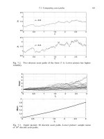
Computational example We used our three finite difference methods to value
a European put option with parameters E = 4, σ = 0.3, r = 0.03 and T = 1.
We truncated the asset range at L = 10. Since the exact value is known from
the Black–Scholes formula (8.24), we may check the error. We focused on the
maximum error at time zero:
err
0
:= max
1≤j ≤N
x
−1
|V
N
t
j
− V ( jh,τ = T )|. (24.9)
With N
x
= 50 and N

t
= 500, so k = 2 × 10
−3
and h = 0.2, we found that
err
0
= 1.5 ×10
−3
for FTCS and err
0
= 1.7 ×10
−3
for BTCS. With Crank–
Nicolson we were able to reduce N
t
to 50, so k = 2 × 10
−2
, and still get a
comparable error, err
0
= 1.6 ×10
−3
. ♦
Our treatment of stability and convergence of finite difference methods in
Chapter 23 does not carry through directly to this section, since the PDE (24.1)
has nonconstant coefficients and includes a first order spatial derivative. However,
similar conclusions may be drawn; see Section 24.5.
24.3 Down-and-out call example
To illustrate the flexibility of finite difference methods, we turn to the down-and-
out call defined in Section 19.2. We know that the PDE holds for B ≤ S. Hence, we

may truncate this to B ≤ S ≤ L and use a grid of the form {B + jh, ik}
N
x
, N
t
j=0,i=0
,
where h = (L − B)/N
x
. The FTCS scheme (24.6) becomes
V
i+1
j
− V
i
j
k
−
1
2
σ
2
(B + jh)
2

V
i
j+1
− 2V
i

j
+ V
i
j−1

h
2
−r(B + jh)

V
i
j+1
− V
i
j−1
2h

+rV
i
j
= 0
and the corresponding BTCS version is
V
i+1
j
− V
i
j
k
−

1
2
σ
2
(B + jh)
2

V
i+1
j+1
− 2V
i+1
j
+ V
i+1
j−1

h
2
−r(B + jh)

V
i+1
j+1
− V
i+1
j−1
2h

+rV

i+1
j
= 0.
24.4 Binomial method as finite differences 261
As before, these may be written in the matrix–vector forms (23.9) and (23.11), and
the Crank–Nicolson method is given by (24.8).
The τ = 0 condition (19.2) specifies V
0
j
= max(B + jh − E, 0) and the
left-hand boundary condition (19.1) gives V
0
i
= 0. At the right-hand boundary,
a reasonable approach is to argue that, since S is large, the asset is very unlikely to
hit the out barrier, so V
i
N
x
= C(L,τ)may be imposed, where C(S, t) denotes the
European call value.
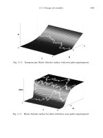
Computational example For the case B = 2, E = 4, σ = 0.3, r = 0.03 and
T = 1weused Crank–Nicolson to value a down-and-out call. In this case the
exact solution (19.3) may be used to check the error. With the asset domain
truncated at L = 10, and with N
x
= N
t
= 50, we found the maximum time-zero
error (24.9) to be err

0
= 1.1 ×10
−3
. ♦
24.4 Binomial method as finite differences
Looking back to Chapter 16, we see some similarities between the binomial and
finite difference methods:
• both work with discretizations of the time and asset domains,
• both advance in the time direction,
• both are designed to be more accurate as the discretization is refined.
The binomial method works in backward time – starting with option values at
t = T and finishing with a value at t = 0 and S = S
0
. The finite difference meth-
ods are more general, in that they produce option values at all grid-points {jh, ik};
in particular, at time zero, option values are available for all initial asset prices
0, h, 2h, ,L.Nevertheless, it should seem plausible that the binomial method
may be regarded as some explicit finite difference scheme that has been customized
to produce a single time-zero option value. In this section we explain how the con-
nection can be made concrete.
Starting with (8.15), we make the transformation X = log S, which produces
the constant coefficient PDE
∂V
∂t
+
1
2
σ
2
∂

2
V
∂ X
2
+ (r −
1
2
σ
2
)
∂V
∂ X
−rV = 0.
We then let V = e
rt
W . This has the effect of eliminating the zeroth derivative
term, to give
∂W
∂t
+
1
2
σ
2
∂
2
W
∂ X
2
+ (r −

1
2
σ
2
)
∂W
∂ X
= 0, (24.10)
262 Finite difference methods for the Black–Scholes PDE
see Exercise 24.4.
Now, applying a backward difference formula for the time derivative and central
differences for the space derivatives in (24.10) leads to the finite difference formula
W
i+1
j
− W
i
j
k
+
1
2
σ
2

W
i+1
j+1
− 2W
i+1

j
+ W
i+1
j−1
h
2

+ (r −
1
2
σ
2
)

W
i+1
j+1
− W
i+1
j−1
2h

= 0. (24.11)
Setting h
2
= σ
2
k has the effect of eliminating the W
i+1
j

terms in (24.11), and the
formula then reduces to
W
i
j
= p

W
i+1
j+1
+ (1 − p

)W
i+1
j−1
, (24.12)
where p

=
1
2

1 +
√
k(r/σ − σ/2)

.Transforming back to V we find that
V
i
j

= e
−rk

p

V
i+1
j+1
+ (1 − p

)V
i+1
j−1

. (24.13)
Comparing (24.13) and (16.3), we see that the binomial method corresponds
to using an explicit finite difference method on a transformed version of the
Black–Scholes PDE. The finite differences are applied on a sub-grid, as illus-
trated in Figure 24.1. The coupling h
2
= σ
2
k puts the method on the very cusp
of von Neumann instability, see Exercise 24.5, which explains the undesirable but
noncatastrophic oscillations observed in Section 16.4.
24.5 Notes and references
As we mentioned in Chapter 23, it is possible to convert the Black–Scholes PDE
for European calls and puts into the heat equation form (23.2). Hence, it is perfectly
reasonable to convert to that form before applying a finite difference method. We
showed how to work directly with the Black–Scholes version (in reverse time)

because in the case of more complicated options such a transformation may not
be possible. We chose to discretize the spatial first derivative ∂V /∂ S in (24.1) by
a central difference. An alternative that is better in the case where the volatility
is very small is upwind differencing; see (Iserles, 1996; Mitchell and Griffiths,
1980; Morton and Mayers, 1994; Strikwerda, 1989).
The texts (Clewlow and Strickland, 1998; Kwok, 1998; Wilmott, 1998; Wilmott
et al., 1995; Seydel, 2002) are good sources for more details about the application
of finite differences to option valuation.
We saw in Chapter 18 that the problem of valuing an American option can be
couched in terms of a linear complementarity problem. It is possible to develop