The Financial Times Guide to Options: The Plain and Simple Guide to Successful Strategies (2nd Edition) (Financial Times Guides)_3 pot

30 Part 1

Options fundamentals
(a) $55 ×
60
/
360
× 0.05 = $0.46 interest added to call price
(b) $0.35 dividend subtracted from call price
(c) $0.46 – 0.35 = $0.11, total added to call price
Note that the price of the stock is not a factor in this calculation. In fact,
DuPont was trading at 57 at the time of this example. There is a difference
of opinion, however. Some traders think that the current price of the stock
is a more accurate basis from which to calculate the interest rate compo-
nent of the option. Practically speaking, the difference between these two
methods is not significant unless the options are far out-of-the-money
with many days until expiration. Again, an options model accounts for
this. More important would be a change in the dividend or the interest
rate until expiration. Also note that unless special circumstances occur
with respect to dividends and interest rates, these pricing components are
far less significant than the volatility component.
Puts on stocks have the opposite pricing characteristics to calls with
respect to cost of carry and dividends. Purchased calls and puts on stocks
are paid for in cash up-front on most exchanges. Sold or short options,
however, are margined because short calls incur potentially unlimited risk,
and short puts incur extreme risk.
Options on stock indexes
A stock index is a proxy for all the stocks that comprise it. Calls and puts
on a stock index are priced according to the cost of carry of the index,
and the amount of dividends contained in the index. The costs of carry

and dividends are added and discounted in the same manner as options
on individual stocks. These options are also paid for in cash.
Long and short options positions
In practice, once a call or put is bought, it is considered to be a long
options position. ‘I’m long 10, June 550 puts,’ you might say. Conversely,
a call or put sold is considered to be a short options position. ‘I’m too
short for my own good,’ means that you have sold too many calls or puts,
or both, for your peace of mind.
It may be helpful to think that when the terms ‘long’ and ‘short’ are
applied to options, they designate ownership. The same terms applied to
a position in the underlying designate exposure to market direction. To
be short puts is to be long the market, i.e. you want the market to move
upward. The following chapter on deltas clarifies this.

3

Pricing and behaviour 31
Exercise and assignment
In practice, most options are not held through
expiration. They are closed beforehand because
the holders of options do not want to take deliv-
ery of the underlyings. The exceptions are options
on stock indexes and options on short-term interest rate contracts such as
Eurodollars. In these contracts, no delivery of an underlying is involved.
Long and short options positions that are in the money at expira-
tion will be converted into underlying positions through exercise and
assignment, respectively. The clearing firms manage this procedure. The
resulting positions are similar to those stated at the end of Chapter 2
under a comparison of calls and puts (page 24). There are slight differences
for each type of contract.

Stocks
Through exercise, the holder of a long call will buy, at the strike price, the
number of shares in the underlying contract. Through assignment, the
holder of a short call will sell the shares. If the short call holder does not
own stock to sell, he will be assigned a short stock position.
Through exercise, the holder of a long put will sell, at the strike price, the
number of shares in the underlying contract. If the long put holder does
not own shares to sell, he will be assigned a short stock position. Through
assignment, the holder of a short put will buy the shares.
Futures
Through exercise, the holder of a long call will acquire, at the strike price,
a long futures position in the underlying. Through assignment, the holder
of a short call will acquire a short futures position at the strike price. On
many futures exchanges, an options contract expires one month before its
underlying futures contract.
For example, expiration for options on November soybeans at the
Chicago Board of Trade (CBOT) normally occurs on the third Friday in
October. If on the day of expiration the November futures contract set-
tles at 552, then the holder of a long November 550 call will exercise to a
long November futures position at the price of 550. The holder of a short
November 550 call will be assigned a short November futures position
at a price of 550. In this case the former long call holder obviously has a
In practice, most
options are not held
through expiration

32 Part 1

Options fundamentals
credit of 2, but he may have originally paid more or less than that for his

November 550 call.
Through exercise, the holder of a long put will acquire, at the strike price,
a short futures position in the underlying. Through assignment, the
holder of a short put will acquire a long futures position at the strike price.
For example, if on the day of expiration the November soybeans futures
contract settles at 552, then the holder of a long November 575 put exer-
cises to a short November futures position at a price of 575. The holder of
a short November 575 put is assigned a long November futures position at
575. The 23 credit for the former long put holder is no indication of the
price at which he originally traded the option.
Cash settled contracts: stock indexes and short-term
interest rate contracts
Through exercise, the holder of a long call will receive the cash differ-
ential between the price of the index or underlying and the strike price
of the call. Through assignment, the holder of a short call will pay the
cash differential.
For example, if at expiration the OEX settles at 527.00, the holder of an
expiring long 525 call position receives 2.00, while the holder of an expir-
ing short 525 call position pays 2.00. The contract multiplier for the OEX
is $100, so in this case $200 changes hands.
Through exercise, the holder of a long put will receive the cash differential
between the strike price of the put and the price of the index or under-
lying. Through assignment, the holder of a short put will pay the cash
differential.
For example, if at expiration the OEX settles at 527.00, the holder of an
expiring long 530 put position receives 3.00, while the holder of an expir-
ing short 530 put position pays 3.00.
The same procedures apply to short-term interest rate contracts such as
Eurodollars and Short Sterling. For example, in either of these contracts if
an option settles one tick in the money, then the long is credited with one

tick times the contract multiplier, and the short is debited one tick times
the contract multiplier. The multiplier for Eurodollars is $25, and the mul-
tiplier for Short Sterling is £12.50.

3

Pricing and behaviour 33
Pin risk
Pin risk is rare, but it is important to know about it. Occasionally, options
expire exactly at-the-money, i.e. the underlying equals the strike price at
the time of expiration. We say that these options, both the call and the
put, are pinned. This causes a problem for options on stocks and options
on futures contracts, but not for options on stock indexes and short-term
interest rate futures contracts.
While there is no immediate profit to be made from exercising these
options, those who hold them may have a short-term directional outlook
for the underlying that warrants exercising them.
For example, if the expiration price of XYZ is 100, the owner of a 100 call
may exercise because he thinks that XYZ will increase in price during the
next trading session, or he may simply want to own it while risking a short-
term decline. The owner of a 100 put may exercise for the opposite reasons
.
The problem lies with the holder of a short position in either of these
options. He may or may not be assigned a position in XYZ. The assign-
ment process is carried out on a random basis by the clearing firms. If the
short option holder is assigned, he will be notified by the opening of the
next trading session. If as usual he does not want to keep a position in
XYZ, he will need to make an offsetting buy/sell transaction at the open-
ing. If the market opens against him, he will cover his position at a loss.
There is no pin risk with cash settled index options such as the OEX and

the FTSE-100 because with these contracts there is no underlying futures
contract or quantity of shares to be assigned, or to exercise to. The same
is true of most short-term interest rate contracts such as Eurodollars and
Short Sterling.
How to manage pin risk
If you are short an option that is close to the underlying with a week until
expiration, it is advisable to buy it back rather than ring the last amount of
time decay from it and risk an unwanted position in the underlying. If you
wait until the morning of expiration, you may find that you are joined by
others with the same position, and you may be forced to pay up to get out.

34 Part 1

Options fundamentals
European versus American style
An option is European style if it cannot be exercised before expiration.
The only way to close this style of option before expiration is to make the
opposing buy/sell transaction. One example is the SPX options on the
Standard and Poor’s 500 Index (S&P 500) traded at the CBOE. Another
example is the ESX options (at the 25 and 75 strikes) on the Financial
Times 100 Index (FTSE-100) traded at the London International Financial
Futures and Options Exchange (LIFFE).
Also available is the American-style option, which can be exercised at any
time before expiration. If such an option becomes so deeply in-the-money
that it trades at parity with the underlying, then it has served its purpose
and represents cash tied up. As a result, it can be sold, or it can be exer-
cised to a position in the underlying stock or futures contract. In the case
of a stock index, such as the OEX, it can be exercised for the cash differen-
tial. Most stock options and futures options are American style.
Black–Scholes and other models

The Black–Scholes options pricing model was the first to succeed. By itself
it practically created an industry. It assumes that the option is held until
expiration. This model is therefore appropriate for European-style options,
but it is less appropriate for American-style options. For index options sub-
ject to early exercise, it must be, and has been, modified significantly.
Most options models assume that volatility is constant through expira-
tion, which it seldom is. This brings challenges to both options buyers and
options sellers. These challenges are discussed later in this chapter.
For more on models and their assumptions please refer to the reading list
given at the end of the book.
Early exercise premium
Because American-style options can be exercised before expiration, those
in-the-money will often contain an additional early exercise premium.
This is not a significant amount for most options on futures contracts. It
is more significant for puts on individual stocks because they can be exer-
cised to sell stock and as a result, interest is earned on the cash.

3

Pricing and behaviour 35
Early exercise premium is a highly significant amount for in-the-money
index options such as the OEX options on the S&P 100 traded at the
CBOE. The reason is that at the end of each trading session, this contract
closes at a different time from its index. Their in-the-money options, espe-
cially their puts, can be driven to parity with the cash index, and can then
become an exercise. To be assigned in this manner often results in a loss.
It is advisable not to sell, or have a short position in, the in-the-money
options of this and similar contracts.
Conversely, because of the potential for early exercise, long out-of-the-
money or at-the-money positions in the above two contracts can profit

significantly. As these options become in-the-money, their early exercise
premium increases drastically. Holders of these options then profit twofold
.
A trader’s story
This brings to mind a story concerning risk and early exercise premium.
I have a personal rule with American styled index options, and that is
always to cover a short position when it becomes 0.50 delta. I made this
rule after one or two incidents when I was short the former FTSE-100
American styled options
3
and they went deep in-the-money on me. Their
early exercise premium mounted, and I became reluctant to pay up in
order to buy them back. I lost more sleep than usual, and then eventu-
ally, a few days or weeks later, they became an exercise at the close. As a
result, I lost my hedge, i.e. I was no longer delta neutral, which is what all
market-makers strive to be. The next morning at the opening, the market
moved against me and I took a loss.
One or two incidents such as this are not serious, but I could see the
potential for serious damage in a highly volatile market. It was then that I
decided on my rule. Subsequently, I paid up whenever I had a short posi-
tion that went to 0.50 deltas. This wasn’t often, but it seemed as if it was
because it always cost me. Anyway, that was the price of a good night’s
sleep, or just a better night’s sleep.
A year or so later, during mid-1997, the emerging market crisis started to
develop. At first, the US seemed to ignore it, and that held London up.
Still, I thought it was time to buy a little extra premium in case the US
changed its mind. The extra premium cost me in time decay, especially
3
These options are no longer listed.

36 Part 1

Options fundamentals
because the FTSE implied was around 20 per cent. In the back of my mind
was, and always is, 19 October 1987.
In October 1997 the UK market started to weaken because of its expo-
sure to Hong Kong, and one day towards the close, I found myself short
a number of 4800 puts which were at-the-money, or 0.50 deltas. A rule
is a rule, I said, which was some consolation for the amount I paid up to
buy them back. I was now longer premium than I generally like to be, and
because we were at the close, I knew I was going to bear the cost of the
time decay.
That night the US cracked. The next morning, the BBC news was calling
for serious losses in London, and I knew there were going to be casual-
ties at the opening. I arrived early at the office, and I had my clerks do
an extensive risk analysis, though I knew, as all market-makers do, that at
a time like this, options theory takes a back seat. I went to the floor and
wedged my way into the crowd, and I waited, knowing that I was covered.
The bell sounded and the shouting began, and after a few brief stops the
FTSE landed at 4400. The traders who were short options were screaming
to buy them back, paying any price from those willing to sell. The implied
volatility leaped to 70 per cent before settling down to a cool 50 per cent
after the opening. I made few trades that day, but they were the ones I
wanted to make. I had my best day ever.
One lesson from this is obvious. Make a plan
to cover your risk and stick to it. Your goal here
is not to make money but to avoid taking a seri-
ous loss. Had I not covered my short options over
the course of a year or more, I would have been one of the casualties. My
profit on that day more than offset all my days of paying up.

Another lesson is that by covering risk, you leave your mind clear to deal
with the circumstance at hand. You can make rational trading decisions.
This is equally true for an extraordinary event or for a more routine trad-
ing day.
Make a plan to cover
your risk and stick to it

4
Volatility and pricing models
The most sophisticated and the most significant aspect of options pricing
is that of volatility. After all, the primary purpose of options is to hedge
exposure to market volatility. Increased market volatility leads to increased
options premiums, while decreased market volatil-
ity has the opposite effect. Although a thorough
review of volatility involves a study of statistics, a
layman’s explanation is practical and sufficient for
the purpose of trading options.
Volatility is generally described in terms of normal price distribution. On
most days, an underlying settles at a price that is not very different from
the previous day’s settlement. Occasionally, there occurs a large price
change from one day to the next. One can safely say that the greater the
price change, the less frequent its occurrence will be.
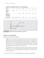
A typical set of price changes for an underlying can be graphed with a bell
curve (see Figure 4.1).
The bell curve places each day’s closing price at the centre, and plots
the next closing day’s price to the right or left, depending on whether
the next day’s price is upward or downward, respectively. The x-axis
denotes the magnitude of the price changes, and the y-axis denotes
their frequency.
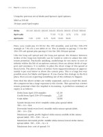
Some underlying contracts routinely have greater daily price changes than

others. They are said to be more volatile. In these cases their bell curves
indicate greater price distribution by exibiting a lower, flatter curve. A
particular contract may also undergo periods of higher volatility. In both
cases the bell curve becomes more like the example shown in Figure 4.2.
The most sophisticated
and the most significant
aspect of options pricing
is that of volatility

38 Part 1

Options fundamentals
The bell curve is a helpful way of visualising the concept of volatility. It
illustrates the need for higher options prices due to higher volatility.
Normal price distribution is similar to waiting for public transport. In
normal circumstances, the bus appears shortly before or after you arrive
at the bus stop. Occasionally, the previous bus has already departed some
time ago, and the next bus arrives at the stop just as you do. At other
times, you just miss the bus, and you need to wait longer than usual.
Number of price changes
Price decrease XYZ Price increase
Figure 4.1
Low volatility
Number of price changes
Price decrease XYZ Price increase
Figure 4.2
High volatility

4


Volatility and pricing models 39
Unfortunately, normal circumstances, like normal markets, are themselves
unusual. Arrivals and departures are subject to a variety of traffic, weather
and professional complications, making it difficult to anticipate bus move-
ments. Sometimes, the street is bumper to bumper with buses. At other
times, you may wait for 20 or more minutes in the rain, and then find
yourself passed by a bus with a sign that says ‘Out of Service’. At these
times you are at the ends of the bell curve.
There are two types of volatility used in the options markets: the histori-
cal volatility of the underlying, and the implied volatility of the options
on the underlying.
Historical volatility
The historical volatility describes the range of price movement of the under-
lying over a given time period. If, for a certain time period, an underlying’s
daily settlement prices are three to five points above
or below its previous daily settlement prices, then
it will have a greater historical volatility than if its
settlement prices are one to two points above or
below. Historical volatility is concerned with price
movement, not with price direction.
Properly speaking, volatility itself is calculated as a one-day, one standard
deviation move, annualised. The annualised figure is used in computing
historical volatility. For example, a stock, bond or commodity with a vola-
tility of 20 per cent has a 68 per cent probability of being within a 20 per
cent range of its present price one year from now; and it has a 95 per cent
probability of being within a 40 per cent range of its present price one year
from now. If XYZ is currently at 100 and the current historical volatility is
20 per cent, then we can be 68 per cent certain that it will be between 80
and 120 one year from now. We can be 95 per cent certain that XYZ will
be between 60 and 140 one year from now.

Most trading firms have mathematical models to calculate volatility, but
for most underlyings there is a simplified way to calculate an annualised
volatility based on a day’s price movement.
An annualised volatility for an underlying can be computed by multiply-
ing the day’s percentage price change by 16.
1
For example, if XYZ settles
The historical volatility
describes the range of
price movement of
the underlying over a
given time period
1

16 is the approximate square root of 250, the approximate number of trading days in a year.

40 Part 1

Options fundamentals
at 100, and the next day it settles at 102:
2
/
100
= 2%. 2% × 16 = 32% annu-
alised volatility. Note that if on the following day XYZ retraces to 100:
2
/
102

= 1.96%. 1.96% × 16 = 31.36% annualised volatility.

This way of calculating volatility is, as mentioned before, simplified, but it
will provide insight into how price changes and the value of the underly-
ing affect the volatility calculation. The above formula is insufficient for
short-term interest rate contracts such as Eurodollars, where the volatility
calculation should be based on the change in the yield or interest rate, and
not on the change in the underlying futures contract.
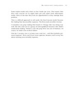
Volatility fluctuates from day to day, but over a time period it often trends
up or down, or remains in a range. In order to put daily volatility fluctua-
tions in perspective, they are averaged into time intervals of 10, 20, 30 days
or more. This process of averaging creates a useful historical volatility. It is
similar to the more familiar moving average of daily settlement prices
.
Because markets frequently change their volatility levels, and because
options are short-term investments, many traders use a 20-day average
6800
6700
6600
6500
6400
6300
6200
6100
6000
5900
5800
5700
5600
5500
5400
5300

5200
5100
5000
4900
4800
4700
4600
4500
4400
4300
4200
4100
4000
D LFTY FTSE-100
F
M A M J J A S O N
11.00
12.00
13.00
14.00
15.00
16.00
17.00
18.00
19.00
20.00
21.00
22.00
23.00
24.00

25.00
26.00
27.00
28.00
29.00
30.00
32.00
33.00
34.00
35.00
36.00
37.00
38.00
39.00
31.00
Figure 4.3
Chart of historical volatility of FTSE-100 index compared to daily
price changes, January–November 1998
Source: FutureSource – Bridge.

4

Volatility and pricing models 41
in order to compute their historical volatility. For longer-term options it
is beneficial to examine the 20-day historical volatility over longer time
periods, perhaps a year or more. In markets that are undergoing a sudden
change of volatility, a five-day average or less may be used for near-term
contracts. It is particularly useful to know what a contract’s historical vola-
tility can be under extraordinary circumstances, both active and quiet. See
Figure 4.3 for an example.

Pricing models
Once the historical volatility is known, it becomes
an input for an options pricing model. The pri-
mary model used in the options industry is the
Black–Scholes model; almost all other models used
are variations of it. This model has been revised
over the past 35 years or so in order to price options on different underly-
ings, but it remains the foundation of the business.
2
The other pricing inputs are those already discussed:
O
strike price of the option
O
price of the underlying
O
time until expiration
O
short-term interest rate
O
dividends
O
volatility, historical or implied.
With these inputs the model yields an option price which can become a
basis from which to trade. If we compare this option price to its current
market price, however, we will probably find a discrepancy. The reason for
this is simply a difference between theory and practice.
Implied volatility
Although a theoretical value for an option can be determined by the his-
torical volatility, an option’s market price is determined by supply and
2

There are many books that discuss the differences between options models. Needless to
say this topic requires an extensive maths background. See the bibliography for recom-
mended readings.
Once the historical
volatility is known, it
becomes an input for an
options pricing model

42 Part 1

Options fundamentals
demand. An options market accounts for past price movement, but it also
tries to anticipate future price movement. The market price of an option,
then, implies a range of expected price movements for the underlying
through expiration.
If we insert the market price of the option into the pricing model, and
if we delete the former historical volatility, the model substitutes another
volatility number, the implied volatility of the option.
This implied volatility can then be used as the implied volatility to calcu-
late market prices of options at other strike prices within the same contract
month. As a result, market prices of options spreads can also be calculated.
For example, if the December Corn futures contract is at 220,
3
and the
December 220 calls, with 60 days until expiration, are priced at 7 ($350),
an options model can calculate that these calls have an implied volatility
of 20 per cent. If the demand for these options bids up their price to 10.5
($525), while at the same time the price of the underlying and the days
until expiration remain constant, the model will calculate that they have
an implied volatility of 30 per cent.

If demand has bid up the 220 calls, then the 240 calls are also worth more
because they are a hedge for underlying price movement as well. The last
traded price of the 240 calls may have been 1.375 but that was before the
220 calls became bid up. Suppose we want to estimate the new theoretical
value for the 240 calls.
If we know that the 220 calls have increased their implied to 30 per cent,
we can assume that the implied for all the options, including the 240 calls,
has increased to 30 per cent.
4
We can assume this because the market is
implying a new volatility for the underlying through expiration, and all
the options will be priced to account for it.
We then insert the 30 per cent implied into the options model, and it
yields a price of 3.375 ($193.75) for the December 240 calls.
You can experiment with the effect of implied volatility changes on
options prices by using an options calculator. Several options’ websites,
including cboe.com, offer one of these. In fact, anyone who seriously
wants to learn about the effects of all the options variables on options
prices should spend a minimum of several hours with this device.
3
Corn is now priced much higher, but this example still holds true.
4
This assumption becomes modified with respect to volatility skews, which are discussed
in Part 3.

4

Volatility and pricing models 43
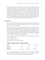
Comparing historical and implied volatility
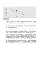
Historical and implied volatility move in tandem; they seldom coincide.

Figure 4.4 compares the historical and implied volatilities for January
Crude Oil, traded at the New York Mercantile Exchange (NYMEX).
5
Here,
the dotted line is the historical volatility and the solid line is the implied
volatility.
This chart can be interpreted in at least two ways.
Because it is an indicator of expected price move-
ment for the underlying, the implied volatility
can be seen as the leader of historical volatility.
Conversely, the historical volatility can be seen as the trend volatility of
the underlying, to which movements in the implied volatility eventu-
ally return. Again, this kind of analysis is similar to that associated with
moving averages and trendlines. The study of volatility is a form of techni-
cal analysis.
5
A great chart from the start of the bull market in commodities. It shows perfectly how
the implied volatility can anticipate an increase in the historical volatility.
10
20
30
40
50
260 235 210 185 160 135 110 85 60 35
Days to Options Expiration v. Volatility (percent)
Solid line Implied Volatility
Figure 4.4
Historical and implied volatilities, January Crude Oil 1998

Source: pmpublishing.com.

The study of volatility
is a form of technical
analysis

44 Part 1

Options fundamentals
Conventional usage
Although it is confusing, in the options markets the term ‘volatility’ can
refer to the daily, historical, or implied volatility. But when an options
trader says ‘Exxon’s at 20 per cent,’ he is referring to the implied volatility
of the front-month, at-the-money call and put. This is the basis of the Vix
contract at the CBOE.
Risk/return
By now, it should be apparent that volatility can be traded in its own
right, independently of market direction. There are many approaches to
this, and several are discussed in later chapters. For now, bear in mind that
if the volatility of an underlying contract increases or decreases, the vola-
tility component of an option will likely increase or decrease respectively.
Because volatility can trend, there is a risk/return potential associated
with volatility direction. Like more conventional kinds of directional trad-
ing, an options trader can take a position that follows the volatility trend,
or not. The options buyer is actually a volatility buyer, while the options
seller is the opposite.
For the volatility buyer, the potential return is the increased volatility
component, or time premium, of the option as the underlying becomes
more active. He can profit significantly if the underlying makes an unex-
pected, large move. The volatility buyer’s major risk is that the underlying
may suddenly come to a halt, and that options premiums collapse.
For the volatility seller, the potential return is the decreased volatility

component of the option as the underlying becomes less active. He can
profit significantly if the underlying quickly settles into a range. The vola-
tility seller’s major risk (and nightmare) is that an unexpected event will
cause the underlying to move sharply while options premiums explode.
The main problem for options traders is to anticipate changes in volatility.
It is comparable to the problem of price direction for stock or commodity
traders.
Traders and the bell curve
The bell curve can be a useful reference when evaluating your perfor-
mance. Please refer to Figures 4.1 and 4.2 earlier. Imagine that profitable

4

Volatility and pricing models 45
days fall to the right of the vertical dotted line (the mean) while loss days
fall to the left.
Now let’s assume that you’ve survived your first year or so, and that
you’ve established a trading style. Some traders have P/L swings like the
curve in Figure 4.1: they are nip and tuck traders. They try to make small
profits and take small losses while earning a good living. Their results are
not spectacular, but they don’t take a lot of risk either.
Other traders have P/L swings like the curve in Figure 4.2. They take more
risk. On the profit days they are handsomely rewarded. On loss days, they
have their risk managers emailing their résumés.
All traders have occasional large P/L swings, i.e. further from the mean.
Just because a trader makes a large profit doesn’t necessarily mean that
he’s a hero, and conversely, if he takes a big loss, it doesn’t mean that he’s
a bum. Traders are like underlying contracts: they have profit swings that
resemble standard deviation moves.
Many people in the industry, including, it seems, senior management

of some very large banks, insurance firms and hedge funds, don’t have a
practical understanding of the bell curve. Keep the bell curve in mind.
A final note
The volatility calculation is based on statistical analysis of asset price
movement. It has the benefit of a great deal of data, but like any other
form of analysis, it cannot predict the future. Ultimately, it is the most
comprehensive means of determining the value of an option.
A thorough understanding of volatility requires research and experience,
but even a basic understanding can be profitable for the options trader.
You may wish to reread this chapter as you work through this book.


5
The Greeks and risk
assessment: delta
Because there are several components that contribute to the price of an
option, it is essential to understand how each of these components can be
affected by changes in the market. Short-term interest rates and dividends,
especially with respect to a stock index, are fairly predictable. The three
major variables that affect an option’s price are:
■
a change in the underlying
■
the passage of time
■
a change in the implied volatility.
Options theory is able to quantify exposure to these variables. The terms
that are applied to the calculations are borrowed from other mathematical
fields, and they are Greek:
■

delta and gamma express exposure to a change in the underlying
■
theta expresses exposure to the passage of time
■
vega expresses exposure to a change in the implied volatility.
‘The Greeks’, as they are called, are invaluable
aides in determining the risk/return potential of
an options position. They are the fundamental
parameters of risk assessment.
Delta
Delta is the amount that an option changes with respect to a small change
in the underlying.
‘The Greeks’, are
invaluable aides in
determining the risk/
return potential of an
options position

48 Part 1

Options fundamentals
If an option is so deeply in-the-money that it is at parity with the under-
lying, its price will change one for one with the underlying. Its delta is
therefore 1.00. Traders often say that this option has a ‘one-hundred delta’
because it has a 100 per cent correlation with the underlying.
An option that is at-the-money changes price at half the rate of the under-
lying, and therefore has a delta of 0.50. Traders often say that this option
has a ‘fifty delta’.
In an extreme case, an option may be so far out-of-the-money that it is vir-
tually worthless. Practically any change in the underlying can not affect its

price. Its delta is therefore 0.00.
Table 5.1 gives a typical example of a set of options with their deltas for
one contract month:
December Corn at $3.80
90 days until expiration
Implied volatility at 30 per cent
Interest rate at 3 per cent
Options multiplier at $50, so multiply call and put values times $50.
Table 5.1 December Corn at 380
Strike Call value
× $50
Call delta Put value
× $50
Put delta
320 63.00 0.90 3
1
/
4
0.10
340 47.00 0.80 7.00 0.20
360 33
7
/
8
0.67 14.00 0.33
380 22.00 0.53 22.00 0.47
400 15.00 0.40 35.00 0.60
420 8
5
/

8
0.27 48
1
/
2
0.73
440 8
1
/
2
0.19 65
1
/
4
0.81
If the December futures contract moves up by one point, then the 380
call moves up by
1
/
2
point, to 22
1
/
2
; the 380 put then moves down by
1
/
2
point, to 21
1

/
2
. If the December futures contract moves down by 1 point,
then the 380 call moves to 21
1
/
2
and the 380 put moves to 22
1
/
2
.

5

The Greeks and risk assesment: delta 49
Note that the 440 call is priced higher than the 320 put even though they
are equally out of the money. This is because the model assumes that
Corn can rally further than it can break.
1
This is a reasonable assump-
tion, but is it a tradable assumption? In other words, is it true for all price
levels? Is it true under any kind of weather? Note as well that a 380 call
costs 22 × $50 = $1,100.
As an underlying changes, the delta itself changes. A large move in the
underlying can change an option’s status from in-the-money to at-the-
money or out-of-the-money, or vice versa. The option’s delta will change
too radically for the purpose of price assessment. The delta calculation
therefore only applies to a small change in the underlying.
Delta and time decay

The delta of an out-of-the-money option decreases with time. This is
because the probability of the underlying reaching its strike price also
decreases with time. The delta of an in-the-money option increases with
time. This is because the probability of its strike price remaining in the
money also increases with time. The delta of an at-the-money option
remains at 0.50. Table 5.2 is another set of options contracts on the above
underlying; it is the same contract month with fewer days until expiration:
Table 5.2 December Corn at $3.80 × 5,000 bushels
Strike Call value
× $50
Call delta Put value
× $50
Put delta
320 60
1
/
8
0.99
1
/
8
0.01
340 41
1
/
8
0.92 1
1
/
4

0.08
360 24
5
/
8
0.76 4
3
/
4
0.24
380 12
1
/
2
0.51 12
1
/
2
0.48
400 5
3
/
8
0.28 25
1
/
4
0.72
420 1
7

/
8
0.12 41
7
/
8
0.83
440
5
/
8
0.04 60
1
/
2
0.96
1
The calls here can actually be priced higher than I’ve given. This is because I have elim-
inated the volatility skew for the purpose of demonstration. To learn about volatility
skews, turn to Chapter 20.

50 Part 1
■
Options fundamentals
30 days until expiration; implied volatility at 30 per cent; interest rate at
3 per cent; options multiplier at $50.
A comparison of each strike price from Table 5.1 to Table 5.2 demonstrates
the effect of time decay on deltas.
Delta position: equivalence to underlying
A delta position corresponds to a long or short position in the underlying.

For example, a long call has a long delta position which corresponds to
a long underlying position. All the delta correspondences are summarised
below:
■
long call = long delta = long underlying
■
short call = short delta = short underlying
■
long put = short delta = short underlying
■
short put = long delta = long underlying.
A consequence of these correspondences is that a delta becomes
equivalent to a percentage of the underlying contract. One short,
at-the-money call with a 0.50 delta equals half of a short underlying con-
tract. Four such calls equal two short underlyings, and so on.
All the deltas in an options position can then be summarised into a net
delta position. Table 5.3 is an example of a small position.
Table 5.3 Sample options position, December Corn, 90 DTE,
implied at 30%
Long Short Call/put Month/strike Delta per
option
Deltas per
position at
strike (+/–)
5 P December 340 0.20 +1.00
10 P December 380 0.47 –4.70
10 C December 380 0.53 +5.30
10 C December 420 0.27 –2.70
10 C December 440 0.19 –1.90
Net delta position –3.00

5
■
The Greeks and risk assesment: delta 51
Here, an equivalent long underlying position is given a plus sign (+), and
an equivalent short underlying position is given a minus sign (–). The net
delta position of –3.00 is equivalent to an underlying position that is short
three contracts. Remember that this equivalency only applies to a small
move in the underlying.
2
Hedge ratio
Because a net delta position is an equivalent futures position, it can indi-
cate exposure to an unwanted move by the underlying. This exposure
would be hedged simply by buying or selling the number of underlying
contracts needed to create a delta neutral position. As a hedge ratio, the
delta indicates the number of contracts to buy or sell.
For example, an option with a 0.50 delta is hedged by half the amount of
underlying contracts. A position of 10 long, 0.50 delta calls is equivalent
to a position of long five underlying contracts. This position is exposed
to downward move by the underlying, and so may be hedged by selling,
or going short, five underlying contracts. The total delta position is then
zero, or, as we say, the position is delta neutral. For a small move by the
underlying in either direction, the profit/loss of the total position changes
little, if at all.
The hedge ratio is especially useful to risk
managers with large options portfolios. They reg-
ularly adjust their exposure to market direction
with offsetting transactions in the underlying con-
tracts. Suppose you are a risk manager with the
position given in Table 5.3. How do you hedge this position?

3
Delta and probability
A useful way to think of delta is that it indicates the probability of an
option expiring in-the-money. An option that is at-the-money, with a 0.50
delta, has an even chance of expiring in-the-money. By associating delta
with probability, we can determine the market’s assessment of the range
of the underlying until expiration. This can help us decide how much risk
lies in an options position.
2
Occasionally in the options business, the plus sign (+) is used to refer to a call delta and
the minus sign (–) is used to refer to a put delta. This practice confuses the process of cal-
culating a net delta position; it is not used in this book.
3
Buy, or go long, three underlying contracts.
The hedge ratio is
especially useful to risk
managers with large
options portfolios

52 Part 1
■
Options fundamentals
For example, the above December 440 call, with an 0.19 delta, has a 19 per
cent probability of expiring in-the-money, and might be considered a low-
risk sale. The return on the sale of this call would also be low, but this is a
justifiable risk/return scenario for some investors.
On the other hand, a 19 per cent probability of December Corn moving
to 440 by expiration may be the point at which another investor wishes
to cover a short position in the underlying. Although the market currently
indicates that such a move is unlikely, this investor is willing to pay the

small premium that would enable him to retain his short position.
As an indicator of probability, a delta is only as good as the current market
assessment of price movement until expiration. This assessment is contin-
ually subject to new information, and as a result it is continually revised.
Profitable options trading is often a matter of anticipating, or being one
of the first to discern, changes in probability.
Summary of delta
There are four ways to think of delta; the first is the definition, and the
following three are the uses:
■
the rate of change of the option with respect to a small change in the
underlying
■
a percentage of an underlying contract
■
a hedge ratio
■
the probability of an option expiring in-the-money.
Delta is discussed further in Part 3.