Báo cáo toán học: " Resource Allocation for Asymmetric Multi-Way Relay Communication over Orthogonal Channels" potx
Bạn đang xem bản rút gọn của tài liệu. Xem và tải ngay bản đầy đủ của tài liệu tại đây (394.87 KB, 19 trang )
This Provisional PDF corresponds to the article as it appeared upon acceptance. Fully formatted
PDF and full text (HTML) versions will be made available soon.
Resource Allocation for Asymmetric Multi-Way Relay Communication over
Orthogonal Channels
EURASIP Journal on Wireless Communications and Networking 2012,
2012:20 doi:10.1186/1687-1499-2012-20
Christoph Hausl ()
Onurcan Iscan ()
Francesco Rossetto ()
ISSN 1687-1499
Article type Research
Submission date 3 March 2011
Acceptance date 18 January 2012
Publication date 18 January 2012
Article URL />This peer-reviewed article was published immediately upon acceptance. It can be downloaded,
printed and distributed freely for any purposes (see copyright notice below).
For information about publishing your research in EURASIP WCN go to
/>For information about other SpringerOpen publications go to
EURASIP Journal on Wireless
Communications and
Networking
© 2012 Hausl et al. ; licensee Springer.
This is an open access article distributed under the terms of the Creative Commons Attribution License ( />which permits unrestricted use, distribution, and reproduction in any medium, provided the original work is properly cited.
Resource Allocation for Asymmetric Multi-Way Relay Com-
munication over Orthogonal Channels
Christoph Hausl
∗ 1
, Onurcan
˙
I¸scan
1
and Francesco Rossetto
2
1
Institute for Communications Engineering, Technische Universit¨at M¨unchen, 80290 Munich, Germany
2
DLR, Institute of Communications and Navigation, 82234 Weßling, Germany
Email: Christoph Hausl
∗
- ; Onurcan
˙
I¸scan - ; Francesco Rossetto -
;
∗
Corresponding author
Abstract
We consider the wireless communication of common information between several terminals with the help of
a relay as it is for example required for a video conference. The transmissions of the nodes are divided in time
and there is no direct link between the terminals. The allocation of the transmission time and of the rates in all
directions can be asymmetric. We derive a closed form expression of the optimal time allocation for a given ratio
of the rates in all directions and for given signal-to-noise ratios of all channels. For specific channel conditions
that guarantee that the network is not ”too asymmetric” we further obtain a closed form expression of the optimal
rate ratio such that the sum-rate is maximized under the assumption that the time allocation is optimally chosen.
We also show that at least one of the terminals should not transmit own data to maximize the sum-rate, if the
network is ”too asymmetric”.
1 Introduction
1.1 Multi-Way Relaying with Network Coding
Consider a multi-way relay system where N termi-
nals want to exchange their independent information
packets with the help of a half-duplex relay over
time-orthogonalized noisy channels. Such a setup
can be used for example for a video conference be-
tween N terminals on earth via a satellite. The task
of the relay is to efficiently forward its received sig-
nals to all terminals, such that every terminal can
decode the messages of each other terminal. For
this aim, we consider a decode-and-forward scheme
where the relay transmits a network encoded ver-
sion of its received packets. In previous work it
was shown that network coding [1] allows an efficient
bidirectional relay communication [2–4] with higher
throughput than one-way relaying. In this work, we
consider network coding for a multi-way relay sys-
tem, which extends bidirectional relaying to more
than two terminals.
Fig. 1 depicts the multi-way relay communica-
tion model with time-orthogonalized channels. We
consider a strategy where the transmission time is
divided into N + 1 time phases. During the first N
time phases (termed as uplink), the terminals trans-
mit to the relay (the other terminals cannot receive
these signals) and in the last time phase (termed as
downlink), the relay broadcasts packets which can
1
be heard by all other terminals. The key idea to
apply network coding in this setup is that the relay
broadcasts to the terminals a function, for example a
bitwise XOR, of its received packets. The terminals
decode the required packets from the relay transmis-
sion and use their own packet as side information.
This scenario with N = 2 terminals and one relay
is mainly studied in the literature as two-way relay-
ing. For the two terminal-case, the achievable rates
of several strategies were considered in [4–8].
Multi-way relaying was first treated indepen-
dently in [9] and [10]. The authors of [9] focused
on the achievable rate region and the diversity-
multiplexing tradeoff of several strategies with a
half-duplex constrained relay. The authors of [10] fo-
cused on the achievable rate region of several strate-
gies with a full-duplex relay. Moreover, they consid-
ered a more general system model than in [9] that in-
cluded the grouping of terminals into clusters which
is also not considered in our paper. In [11] a scheme
called functional decode-and-forward was proposed
for the multi-way relay channel, where the relay de-
codes and forwards a function of the messages of the
source nodes. The same authors extended their work
also in [12,13]. Another work on multi-way relaying
was done in [14,15] where the authors consider non-
regenerative relaying with beamforming. The same
authors considered similar scenarios with regenera-
tive relaying in [16] and multi-group multi-way relay-
ing in [17,18]. Code design for the multi-way relay
channel with N = 3 terminals and with direct link
between the terminals was considered in [19].
1.2 Contribution of this Paper
We consider scenarios with asymmetric channel
quality and asymmetric data traffic. For example,
such scenarios arise for a video conference via a satel-
lite where some of the terminals have a better receive
antenna and desire a high received data rate to show
the video on a large screen whereas the other termi-
nals have a smaller receive antenna and require a
lower data rate.
The main contribution of this work is the opti-
mization of the time and rate allocation parameters
for such setups. This work extends the optimization
parts of [20], where we only considered N = 2 ter-
minals, to an arbitrary number of terminals. This is
the first work which concentrates on the optimiza-
tion of the resource allocation for multi-way relay
systems with asymmetric channels. Moreover, we
obtain insights about the scalability of the network
coding gain with the network size.
After introducing the system model in Section
2, we consider in Section 3 how to optimally al-
locate the transmission time to the terminals and
the relay and how to optimally allocate the rates of
the terminals such that the sum-rate is maximized.
We first derive a closed form expression of the opti-
mal time allocation for given rate ratios and given
signal-to-noise ratios (SNRs) of all channels. Then,
we show that the optimization of the rate alloca-
tion under the assumption that the time allocation
is optimally chosen can be transformed into a linear
optimization problem that is solvable with computa-
tionally efficient algorithms. Moreover, we obtain a
closed form expression for the rate optimization that
is valid for specific channel conditions that guaran-
tee that the network is not ”too asymmetric”. If the
network is ”too asymmetric”, at least one of the ter-
minals should not transmit own data to maximize
the sum-rate. In Section 4 we provide examples to
show how the optimization can increase the system
performance. Section 5 concludes the work.
2 System Model
2.1 System Setup
Consider a multi-way communication between N
terminals T
i
with 1 ≤ i ≤ N via a relay where each
terminal wants to communicate common informa-
tion to all other terminals. We do not consider pri-
vate information that is only intended for a subset
of all terminals. The information bits of terminal
i are segmented in packets u
i
of length K
i
. The
packets carry statistically independent data. At T
i
,
the bits u
i
are protected against transmission errors
with channel codes and modulators which output the
block x
i
containing M
i
symbols. T
i
transmits x
i
to
the relay with power P
i
in the i-th of the N + 1 time
phases. We consider a time-division channel without
interference between nodes.
The relay demodulates and decodes in the i-th
time phase the corrupted version y
iR
of x
i
to obtain
the hard estimate
˜
u
i
about u
i
. Then, the estimates
˜
u
i
of all terminals are network encoded and modu-
lated to the block x
R
containing M
R
symbols. The
relay broadcasts x
R
to all terminals with power P
R
in the N + 1-th time phase.
T
i
receives the corrupted version y
Ri
of x
R
in the
N + 1-th time phase. Based on y
Ri
and on the own
2
information packet u
i
, the decoder at T
i
outputs the
hard estimates
ˆ
u
j
about u
j
for all j between 1 and
N except for j = i.
The total number of transmitted symbols is given
by M = M
R
+
N
i=1
M
i
. The transmitted rate in in-
formation bits per symbol from T
i
is R
i
= K
i
/M.
The transmitted sum-rate of the system is given by
R =
N
i=1
R
i
= (
N
i=1
K
i
)/M. We define the time
allocation parameters θ
i
= M
i
/M for 1 ≤ i ≤ N and
θ
R
= 1−
N
i=1
θ
i
. Moreover, we define the rate ratios
σ
i
= R
i
/R for 1 ≤ i ≤ N with
N
i=1
σ
i
= 1. Note
that the rate ratios are defined differently compared
to [20]. The block diagram of the system model is
depicted in Fig. 2.
2.2 Channel Model
All channels are assumed to be AWGN channels and
thus the received samples after the matched filter are
y
iR
= h
iR
· x
i
+ z
iR
(T
i
transmits) (1)
y
Ri
= h
Ri
· x
R
+ z
Ri
(R transmits) (2)
with the channel coefficients h
iR
and h
Ri
for 1 ≤
i ≤ N modeling path loss and antenna gains. The
noise values z
k
are zero-mean and Gaussian dis-
tributed with variance N
0
· W/2 per complex dimen-
sion, where W denotes the bandwidth.
The SNRs are given by γ
iR
= P
i
· h
iR
/(N
0
· W )
and by γ
Ri
= P
R
· h
Ri
/(N
0
· W ).
3 Optimization of Time and Rate Allo-
cation
In this section we consider the problem of how to
optimally allocate the transmission time to the ter-
minals and to the relay and how to optimally allocate
the rates of the terminals such that the sum-rate is
maximized. We extend the work in [20] from N = 2
to an arbitrary number of terminals.
3.1 Achievable Rate Region
Assuming the system model given in the previous
section, the data of T
i
can be decoded reliably at all
other terminals, if the following conditions hold for
all i in 1 ≤ i ≤ N:
R
i
≤ θ
i
· C (γ
iR
) (3)
N
j=1, j=i
R
j
= R · (1 − σ
i
) ≤ θ
R
· C (γ
Ri
) (4)
with C(γ) = log
2
(1 + γ) for Gaussian distributed
channel inputs. The conditions in (3) ensure that
the relay is able to decode reliably while the condi-
tions in (4) ensure that the terminals are able to de-
code reliably. The conditions in (4) can be obtained
from [21]. A similar result has been derived in [22]
where more a priori information is assumed than in
our channel model. For N = 2 these conditions are
derived in [5] and [23].
3.2 Optimal Time Allocation
In this section we consider the optimization of the
time allocation parameters θ = [θ
1
θ
2
. . . θ
N
]
T
such
that the sum-rate R is maximized for given rate ra-
tios σ = [σ
1
σ
2
. . . σ
N
]
T
. Formally, the optimiza-
tion is stated as
θ
∗
= arg max
θ
R (5)
subject to
0 ≤ θ
i
≤ 1 ∀i ∈ {1, 2, . . . , N }
0 ≤ θ
R
= 1 −
N
i=1
θ
i
≤ 1
and with
R = min
1≤i≤N
θ
i
σ
i
C (γ
iR
) , (1 −
N
j=1
θ
j
)
C (γ
Ri
)
1 − σ
i
(6)
= min
1≤i≤N
θ
i
σ
i
C (γ
iR
) , (1 −
N
j=1
θ
j
) · a
(7)
whereas a is given by
a = min
1≤k≤N
C (γ
Rk
)
1 − σ
k
(8)
and the arguments of the minimum in (6) follow
from (3), from (4), from R
i
= σ
i
· R and from
θ
R
= 1−
N
i=1
θ
i
. The step from (6) to (7) is done to
ensure that the second argument of the minimization
is independent of i.
3
The solution of the optimization follows by set-
ting the first and the second argument in (7) to
equality for all i with 1 ≤ i ≤ N:
θ
∗
i
σ
i
C (γ
iR
) = (1 −
N
j=1
θ
∗
j
) · a (9)
The optimization can be solved in this way, because
• the first argument increases monotonically
with θ
i
,
• the second argument decreases monotonically
with θ
i
,
• it is guaranteed that the first and the second
argument have a cross-over point for C(γ
iR
) ≥
0 and C(γ
Ri
) ≥ 0.
In order to find the N unknown θ
∗
i
, N equations
are provided by (9). As long as these N equations
are linearly independent, the optimal time allocation
parameters θ
∗
can be obtained by
C(γ
1R
)
σ
1
+ a a · · · a
a
C(γ
2R
)
σ
2
+ a
.
.
.
.
.
.
.
.
.
a
a · · · a
C(γ
N R
)
σ
N
+ a
−1
a
a
.
.
.
a
.
(10)
Eq. (10) can be further simplified by using the
matrix inversion lemma [24]
(B + UAV)
-1
= B
-1
− B
-1
U(A
-1
+ VB
-1
U)
-1
VB
-1
,
where we set A = a, V = [1 1]
1×N
, U = V
T
and
B as a diagonal N × N matrix with C(γ
iR
)/σ
i
as
the i-th diagonal element. Accordingly, the optimal
time allocation parameters θ
∗
i
for all i are given by
θ
∗
i
=
σ
i
C(γ
iR
)
1
a
+
N
j=1
σ
j
C(γ
jR
)
(11)
and the corresponding achievable sum-rate R is
given by
R =
θ
∗
i
σ
i
C(γ
iR
) =
1
a
+
N
j=1
σ
j
C(γ
jR
)
−1
. (12)
This also shows that the matrix in (10) is invertible
if C(γ
iR
) > 0 holds for all i. Moreover, it can be seen
from Eq. (12) that if the uplink capacity C(γ
iR
) of
terminal T
i
is increased, the allocated time for that
terminal decreases. Another interesting observation
is that θ
∗
i
depends on all uplink capacities and only
on one downlink capacity given in (8). It does not
depend on the other downlink capacities.
3.3 Optimal Time and Rate Allocation
Based on the result in the previous section we con-
sider the optimal choice for the rate ratios σ =
[σ
1
σ
2
. . . σ
N
]
T
such that the sum-rate R of the
system is maximized when the time allocation θ =
[θ
1
θ
2
. . . θ
N
]
T
is chosen optimally. Formally, the
optimization is stated as
σ
∗
= arg max
σ
R = arg max
σ
1
a
+
N
j=1
σ
j
C(γ
jR
)
−1
(13)
subject to
0 ≤ σ
i
≤ 1 ∀i ∈ {1, 2, . . . , N }
N
i=1
σ
i
= 1.
The optimization in (13) can be expressed as the
following linear optimization problem [25]:
[σ
∗
b
∗
] = arg min
[σ b]
b +
N
j=1
σ
j
C(γ
jR
)
(14)
subject to
0 ≤ σ
i
≤ 1 ∀i ∈ {1, 2, . . . , N }
N
i=1
σ
i
= 1
0 ≥
1 − σ
i
C (γ
Ri
)
− b ∀i ∈ {1, 2, . . . , N}.
This allows to solve the problem with computation-
ally efficient numerical algorithms. Note that in this
expression b = 1/a is included as additional opti-
mization variable.
The result of a linear optimization problem can
only be given by a vertex [σ
∗
b
∗
] of the polyhedron
defined by the constraints of the linear optimization
problem [25]. We want to take a closer look at one
specific vertex which is optimal for networks that
4
are not ”too asymmetric”. We term this vertex as
[σ
∗
S
b
∗
S
], whereas the i-th element of σ
∗
S
is given by
σ
∗
S,i
= 1 −
(N − 1) · C (γ
Ri
)
N
j=1
C (γ
Rj
)
∀i ∈ {1, 2, . . . , N }
(15)
and the rate
R
∗
S
=
N − 1
N
j=1
C (γ
Rj
)
·
1 −
N
j=1
C (γ
Rj
)
C (γ
jR
)
+
N
j=1
1
C (γ
jR
)
−1
(16)
is achievable at this vertex. The vertex [σ
∗
S
b
∗
S
] is
optimal, if
N
j=1
C (γ
Rj
)
C (γ
jR
)
≤ 1 +
1
C (γ
iR
)
·
N
j=1
C (γ
Rj
)
∧
(N − 1) · C (γ
Ri
)
N
j=1
C (γ
Rj
)
≤ 1
(17)
is valid for all i ∈ {1, 2, . . . , N} whereas ∧ denotes
a logical AND (derivation in Appendix 6.1). We
denote networks where (17) is not fulfilled for any
i ∈ {1, 2, . . . , N} as ”too asymmetric” for full net-
work coding, because the vertex [σ
∗
S
b
∗
S
] is the only
solution of the optimization problem where it is pos-
sible that σ
∗
i
> 0 for all i ∈ {1, 2, . . . , N} (derivation
in Appendix 6.1). That means if (17) is not fulfilled
for any i ∈ {1, 2, . . . , N}, at least one σ
∗
i
is zero.
Those terminals do not transmit any packet at all.
It is also interesting to see that for reciprocal chan-
nels (C (γ
Ri
) = C (γ
iR
) for all i ∈ {1, 2, . . . , N}) both
conditions in (17) are identical.
Although the explicit solution in (15) could be
also obtained numerically with the linear optimiza-
tion, it is worthwhile to express it explicitly, because
Condition (17) is fulfilled for specific networks that
are of practical relevance, for example
• for completely symmetric networks where all
capacities are equal (C(γ
iR
) = C(γ
Ri
) = C for
all i ∈ {1, 2, . . . , N }),
• for ”close-to-symmetric” networks in the
sense that the set of all terminal-indices
{1, 2, . . . , N} is split into the four disjoint sub-
sets N
b
, N
u
, N
d
and N
r
with cardinalities
|N
b
| = N
b
, |N
u
| = N
u
, |N
d
| = N
d
and
|N
r
| = N
r
= N − N
b
− N
u
− N
d
and that
the following properties are fulfilled:
◦ C(γ
iR
) = C(γ
Ri
) = C + δ for all i ∈ N
b
◦ C(γ
iR
) = C + δ and C(γ
Ri
) = C for all
i ∈ N
u
◦ C(γ
iR
) = C and C(γ
Ri
) = C + δ for all
i ∈ N
d
◦ C(γ
iR
) = C(γ
Ri
) = C for all i ∈ N
r
◦ δ is constrained to be in the following in-
terval (derivation in Appendix 6.2):
δ
C
≥ max
−
1
N
d
+ N
b
,
(N
u
+N
b
+1)
2
− 4N
b
− N
u
− N
b
− 1
2N
b
(18)
δ
C
≤ min
1
N − N
d
− N
b
− 1
,
(N
r
+N
d
−1)
2
+ 4N
d
− N
r
− N
d
+ 1
2N
d
(19)
◦ [N
b
> 0], [N
d
> 0], [N
u
+ N
b
< N] and
[N
d
+ N
b
< N].
• for networks with reciprocal channels, where
C(γ
iR
) = C(γ
Ri
) ≤
N
N − 1
C
D
(20)
is fulfilled for all i ∈ {1, 2, . . . , N} whereas
C
D
=
1
N
N
j=1
C (γ
Rj
) describes the average
downlink capacity. Note that Condition (20)
becomes more strict with growing N , because
N
N−1
approaches to 1 and hence the capacities
of the channels should be closer to the average
capacity C
D
in order to fulfill the conditions
given in (17).
• for networks with N = 2 with C(γ
2R
) ≥ C(γ
R2
)
and C(γ
1R
) ≥ C(γ
R1
) (for example for all re-
ciprocal channels).
Moreover, the explicit solution in (15) can be re-
garded as an appropriate initial point for numerical
algorithms.
We want to take a closer look at the optimization
result for N = 2 in order to allow an easier interpre-
tation of the result [20]. Moreover, this allows us to
treat also the cases explicitly in closed form where
5
(17) is not fulfilled. We simplify the notation and
use ρ = σ
2
/σ
1
= 1/σ
1
− 1. The solution of the opti-
mization for N = 2 is given by
ρ
∗
= 0, if ∆
u
< −1/C(γ
R2
)
ρ
∗
→ ∞, if ∆
u
> 1/C(γ
R1
)
ρ
∗
= C(γ
R1
)/C(γ
R2
), else
(21)
with ∆
u
= 1/C(γ
1R
) − 1/C(γ
2R
), where the optimal
rate
R
∗
=
C(γ
1R
) · C(γ
R2
)
C(γ
1R
) + C(γ
R2
)
, if ∆
u
<
−1
C(γ
R2
)
C(γ
2R
) · C(γ
R1
)
C(γ
2R
) + C(γ
R1
)
, if ∆
u
>
1
C(γ
R1
)
C(γ
R2
) + C(γ
R1
)
1 +
C(γ
R2
)
C(γ
1R
)
+
C(γ
R1
)
C(γ
2R
)
, else
(22)
is achievable. For the last case in (21) and (22)
Condition (17) is fulfilled and thus, the optimal rate
allocation and the corresponding rate are given by
(15) and (16), respectively. The optimization of the
other two cases is derived in [20]. We conclude from
(21) that network coding should only be used for
−1/C(γ
R2
) ≤ 1/C(γ
1R
) − 1/C(γ
2R
) ≤ 1/C(γ
R1
) to
achieve the maximum sum-rate. Otherwise the net-
work is “too asymmetric” and it is optimal to com-
municate only in one direction for achieving the max-
imum sum-rate. If network coding should be used,
the optimal rate ratio σ
∗
depends only on the links
from the relay to the terminals. As mentioned pre-
viously, for C(γ
2R
) ≥ C(γ
R2
) and C(γ
1R
) ≥ C(γ
R1
)
the result of the optimization in (21) simplifies and
it is always optimal to use network coding with
ρ
∗
= C(γ
R1
)/C(γ
R2
).
3.4 Reference System without Network Coding
In this section we describe a reference system for the
multi-way relay communication, where no network
coding is used. In this scheme the transmission time
is split into 2N time phases. The first N phases are
the same as in Section 2 and the next N phases are
used by the relay to forward the packets that it re-
ceived in the first N phases to the terminals (During
the N + i-th phase, the received packet from the i-
th phase is broadcasted). For comparison with the
network coding case, we also optimize the time allo-
cation and the rate ratio.
3.4.1 Achievable Rate Region
In this system, the following conditions have to hold
for all i in 1 ≤ i ≤ N in order to ensure a reliable
communication between each terminal [26]:
R ≤
θ
i
σ
i
· C(γ
iR
) (23)
R ≤
θ
i+N
σ
i
min
j∈{1,2, ,N }i
C(γ
Rj
) (24)
3.4.2 Optimal Time Allocation
We first consider the optimization of the time allo-
cation vector θ = [θ
1
θ
2
. . . θ
2N−1
]
T
for a given rate
ratio vector σ = [σ
1
σ
2
. . . σ
N
]
T
. Considering the
conditions in (24), the optimization can be stated as
follows:
θ
∗
= arg max
θ
R (25)
subject to
0 ≤ θ
i
≤ 1, i ∈ {1, 2, . . . , 2N − 1}
0 ≤ θ
2N
= 1 −
2N−1
i=1
θ
i
≤ 1
and with
R = min
1≤i≤N
θ
i
σ
i
· C(γ
iR
),
θ
i+N
σ
i
· min
j∈{1,2, ,N }i
C(γ
Rj
)
(26)
The solution of the optimization can be found
similarly to the one in Section 3.2 by setting the
2N terms in Eq. (26) to equality. We set ev-
ery term in Eq. (26) equal to the very last term
(θ
2N
/σ
N
min
j∈{1,2, ,N −1}
C(γ
Rj
)) and express θ
2N
=
1 −
2N−1
i=1
θ
i
in terms of the sum of all other
θ
i
’s, which at the end gives us 2N − 1 equations
with 2N − 1 unknowns. Without loss of general-
ity, we assume that the notation is chosen such that
C(γ
R1
) ≤ C(γ
R2
) ≤ ·· · ≤ C(γ
RN
) is valid. This im-
plies
C(γ
R2
) = min
j∈{1, ,N }i
C(γ
Rj
) for i = 1 (27)
and
C(γ
R1
) = min
j∈{1, ,N }i
C(γ
Rj
) for i > 1. (28)
6
Then, we can derive with the help of the matrix
inversion lemma that the the solution of the problem
is given by
θ
∗
i
=
s
i
1 − σ
1
C(γ
R1
)
+
σ
1
C(γ
R2
)
+
N
j=1
σ
j
C(γ
jR
)
(29)
with
s
i
=
σ
i
C(γ
iR
)
if 1 ≤ i ≤ N
σ
1
C(γ
R2
)
if i = N + 1
σ
i−N
C(γ
R1
)
if N + 2 ≤ i ≤ 2N − 1
(30)
whereas θ
∗
2N
can be expressed as θ
∗
2N
= 1−
2N−1
i=1
θ
∗
i
and b is given by b = C(γ
R1
)/σ
N
. The corresponding
achievable sum-rate R is given by
R =
θ
∗
i
σ
i
C(γ
iR
)
=
1 − σ
1
C(γ
R1
)
+
σ
1
C(γ
R2
)
+
N
j=1
σ
j
C(γ
jR
)
−1
. (31)
3.4.3 Optimal Time and Rate Allocation
Based on the result in the previous section we con-
sider the optimal choice for the rate ratios σ =
[σ
1
σ
2
. . . σ
N
]
T
such that the sum-rate R of the sys-
tem is maximized when the time allocation θ is cho-
sen optimally. Formally, the optimization is stated
as
σ
∗
= arg max
σ
R
= arg max
σ
1 − σ
1
C(γ
R1
)
+
σ
1
C(γ
R2
)
+
N
j=1
σ
j
C(γ
jR
)
−1
(32)
subject to
0 ≤ σ
i
≤ 1 ∀i ∈ {1, 2, . . . , N }
N
i=1
σ
i
= 1.
One solution of the optimization is given by
σ
∗
1
= 1 (33)
σ
∗
i
= 0 ∀i ∈ {2, 3, . . . , N } (34)
with
R
∗
=
1
C (γ
R2
)
+
1
C (γ
1R
)
−1
(35)
if
1
C (γ
1R
)
+
1
C (γ
R2
)
−
1
C (γ
R1
)
≤
1
C (γ
iR
)
(36)
is valid for all i ∈ {1, 2, . . . , N}.
If (36) is not fulfilled for any i ∈ {1, 2, . . . , N },
then the optimal rate allocation parameter is given
by
σ
∗
j
= 1 (37)
σ
∗
i
= 0 ∀i ∈ {1, 2, . . . , N }/j (38)
with
j = arg min
i∈{1,2, ,N}
1
C (γ
iR
)
= arg max
i∈{1,2, ,N}
C (γ
iR
)
(39)
and
R
∗
=
1
C (γ
R1
)
+
1
C (γ
jR
)
−1
. (40)
This means it is optimal to communicate only in
one direction to maximize the sum-rate. The solu-
tion can be obtained similarly to the derivation in
Section 3.3.
4 Examples
4.1 Example 1
Consider a symmetrical setup with N terminals
where all the channels are of the same quality with
C(γ) = 1 bits per symbol. If the optimization of the
time and rate allocation parameters is done accord-
ing to the previous sections, we obtain for the case
with network coding according to (15), (16) and (11)
σ
∗
i
=
1
N
∀i ∈ {1, 2, . . . , N }, (41)
R
∗
=
N
2N − 1
(42)
and
θ
∗
i
=
1
2N − 1
∀i ∈ {1, 2, . . . , N }. (43)
For the case without network coding we obtain
according to (35)
R
∗
=
1
2
. (44)
The achievable sum-rate R dependent on the
number of terminals N is shown in Fig. 3. It can be
7
seen that R for the case without network coding is
constant, whereas if network coding is applied, the
sum-rate R is always larger compared to the case
without network coding. Another important result
is that the largest gain is achieved for N = 2 termi-
nals and with increasing N the gain due to network
coding decreases. Note that contrary to the con-
sidered transmitted sum-rate, the received sum-rate
((N − 1) · R ) would increase with growing N.
4.2 Example 2
Consider a two-terminal example with C(γ
R1
) = 3,
C(γ
R2
) = 2 and C(γ
2R
) = 1 bits per symbol. Fig. 4
depicts the optimal values ρ
∗
= σ
∗
2
/σ
∗
1
and R
∗
for
network coding and the corresponding values with-
out network coding dependent on C(γ
1R
). Accord-
ing to (21), it is optimal to use network coding with
ρ
∗
= 3/2 for 3/4 < C(γ
1R
) < 2 whereas 3/4 and
2 can b e regarded as network coding thresholds.
If C(γ
1R
) is not between these thresholds, network
coding should not be used to maximize the sum-
rate. By using network coding the optimal sum-
rate can be increased to 0.88 bits per channel use at
C (γ
1R
) = 1.2, while the sum-rate without network
coding is 0.75 bits per channel use. This corresponds
to an increase of 17.5% in spectral efficiency.
4.3 Example 3
Fig. 5 depicts the achievable sum-rate R over the
SNR γ
R1
from R to T
1
in a scenario with N = 5 ter-
minals. All other SNRs are set to γ
R1
+ 10 dB. The
reason for the lower channel receive-quality at T
1
could be a smaller antenna with a lower gain com-
pared to the other terminals. We consider systems
with and without network coding and assume Gaus-
sian distributed channel input distributions. If both
time and rate allocation are optimized, network cod-
ing gains more than 1.4 dB compared to the system
without network coding for a sum-rate of R = 4.0
bits per symbol. If the time allocation is optimized
for an equal rate allocation, network coding gains
more than 1.3 dB for R = 3.0 bits per symbol. For
an equal time and rate allocation, network coding
gains more than 2.5 dB for R = 2.0 bits per symbol.
The systems with the optimal time and rate al-
location perform best and gain for a sum-rate of
R = 2.0 bits per symbol more than 5.3 dB compared
to the corresponding systems with equal rates.
If both time and rate allocation are optimized
and network coding is used, the terminal T
1
with
the weakest relay-terminal channel transmits with
the largest rate. For example, for γ
R1
= 10
dB the optimal allocation vectors are given by
σ
∗
= [0.540 0.115 0.115 0.115 0.115]
T
, θ
∗
=
[0.287 0.061 0.061 0.061 0.061]
T
and θ
∗
R
= 0.4690.
4.4 Example 4
Fig. 6 shows the achievable rates for a scenario sim-
ilar to the previous example with N = 2 terminals.
All other SNRs than γ
R1
are again set to γ
R1
+ 10
dB.
If both time and rate allocation are optimized,
network coding gains more than 4.0 dB compared to
the system without network coding for a sum-rate of
R = 4.0 bits per symb ol. If the time allocation is op-
timized for an equal rate allocation, network co ding
gains more than 3.4 dB for R = 3.0 bits p er sym-
bol. For an equal time and rate allocation, network
coding gains more than 6.9 dB for R = 2.0 bits per
symbol. This confirms the observation in Example
1 that the gain due to network coding is maximized
for N = 2.
The systems with the optimal time and rate al-
location perform best and gain for a sum-rate of
R = 2.0 bits per symbol more than 3.4 dB compared
to the corresponding systems with equal rates.
If both time and rate allocation are optimized
and network coding is used, the terminal T
1
with the
weakest relay-terminal channel transmits with the
largest rate. For example, for γ
R1
= 10 dB the opti-
mal allocation vectors are given by σ
∗
= [0.66 0.34]
T
,
θ
∗
= [0.397 0.206]
T
and θ
∗
R
= 0.397.
The rate for equal time and rate allocation with
network coding changes its pre-log-factor from 1 to
0.5 at γ
R1
= 9 dB because the rate is limited by the
communication to the terminals for γ
R1
< 9 dB and
by the communication to the relay for γ
R1
> 9 dB.
The considered networks in the Examples 3 and 4
are never ”too asymmetric” in the range −10 dB ≤
γ
R1
≤ 15 dB and thus, the explicit expression in (16)
can be always used to calculate R
∗
.
5 Conclusion
We considered communication systems with multi-
ple terminals and one relay where the terminals want
to transmit their packets to each other. We derived
8
closed form expressions for the optimal time allo-
cation. We also obtained a closed form expression
for the optimal rate allocation that is valid for spe-
cific channel conditions that guarantee that the net-
work is not ”too asymmetric”. If these conditions
are not fulfilled we showed that the optimization
can be solved efficiently with linear optimization al-
gorithms. For asymmetric channel conditions, the
sum-rate is larger if we allow the time and rate al-
location to be asymmetric as well. It turns out that
the largest gain due to network coding is obtained
for N = 2 terminals and the gain decreases with
increasing N .
In further work, efficient code design for asym-
metric multi-way relay systems could be considered.
6 Appendix
6.1 Derivation of Optimal Rate Allocation
We want to show under which conditions the vertex
[σ
∗
S
b
∗
S
] whose elements are given according to (15) is
the solution of the optimization in (14). The deriva-
tion follows [25, Chapter 3.1]. First, we transform
the optimization problem in (14) with the help of
slack variables s
i
to its corresponding standard form
which is given by
x
∗
= arg min
x
c
T
· x s.t. A · x = b and x ≥ 0
T
2·N+1
with
x = [σ b s
1
s
2
. . . s
N
]
T
c = [
1
C(γ
1R
)
1
C(γ
2R
)
. . .
1
C(γ
NR
)
1 0
N
]
T
b = [
1
C(γ
R1
)
1
C(γ
R2
)
. . .
1
C(γ
RN
)
1]
T
A =
1
C(γ
R1
)
0 · · · 0 1
0
1
C(γ
R2
)
.
.
.
.
.
. 1
.
.
.
.
.
.
.
.
.
0
.
.
.
0 · · · 0
1
C(γ
RN
)
1
1 1 · · · 1 0
−1 0 · · · 0 0
0 −1 0 · · · 0
.
.
.
.
.
.
.
.
.
.
.
.
.
.
.
0 · · · 0 −1 0
T
whereas 0
l
denotes an all-zero row vector of length
l. The problem contains n = 2 · N + 1 variables with
m = N + 1 equality constraints. A vector x ∈ R
n
is
a vertex if A · x = b is fulfilled and n − m elements
of x are zero [25, Theorem 2.4].
We only consider the vertex x
∗
S
= [σ
∗
S
b
∗
S
0
N
]
T
with s
i
= 0 for all i ∈ {1, 2, . . . , N} which is given
by
[σ
∗
S
b
∗
S
]
T
= B
−1
· b (45)
whereas B is a m × m matrix which consists of the
first m columns of A. This is the only vertex where
no σ
i
with i ∈ {1, 2, . . . , N } is constrained to be
zero, because b = 0 and s
i
= 0 leads to σ
i
= 1 which
would imply σ
j
≤ 0 for j ∈ {1, 2, . . . , N}/i.
The vertex x
∗
S
is optimal if
c
T
− c
T
S
· B
−1
· A ≥ 0
n
(46)
and
B
−1
· b ≥ 0
T
m
(47)
is fulfilled whereas c
S
is the vector which contains
the first m elements of c [25, Chapter 3.1]. The
condition in (46) is for the last N elements equiva-
lent to the left hand side in Condition (17) and the
condition in (47) is for the first N elements equiva-
lent to the right hand side in Condition (17). The
conditions (46) and (47) are always fulfilled for the
other elements. The corresponding solution of the
optimization in (15) follows from (45).
6.2 Derivation of δ-Interval for ”Close-to-
Symmetric” Networks
The first argument of the maximum in (18) follows
from the right hand side of (17) for C(γ
Ri
) = C.
The second argument of the maximum in (18) fol-
lows from the left hand side of (17) for C(γ
iR
) = C.
The first argument of the minimum in (19) follows
from the right hand side of (17) for C(γ
Ri
) = C + δ.
The second argument of the minimum in (19) follows
from the left hand side of (17) for C(γ
iR
) = C + δ.
7 Competing Interests
The authors declare that they have no competing
interests.
8 Acknowledgements
The authors are supported by the Space Agency of
the German Aerospace Center and the Federal Min-
istry of Economics and Technology based on the agree-
ment of the German Federal Parliament (support code
9
50YB0905). C. Hausl is also supported by the EC-
funded Network of Excellence NEWCOM++ (contract
n. 216715). The authors thank Prof. Gerhard Kramer
and Michael Heindlmaier for their helpful comments.
10
References
1. Ahlswede R, Cai N, Li SYR, Yeung RW: Network Infor-
mation Flow. IEEE Transactions on Information The-
ory 2000, 46(4):1204–1216.
2. Yeung RW, Li SYR, Cai N, Zhang Z: Network Coding
Theory, Part I: Single Source, Volume 2. now Publishers
2005.
3. Wu Y, Chou PA, Kung SY: Information Exchange
in Wireless Networks with Network Coding and
Physical-Layer Broadcast. In Conference on Informa-
tion Sciences and Systems (CISS) 2005.
4. Larsson P, Johansson N, Sunell KE: Coded Bi-
directional Relaying. In IEEE Vehicular Technology
Conference 2006:851–855.
5. Kim SJ, Mitran P, Tarokh V: Performance Bounds
for Bi-Directional Coded Cooperation Proto-
cols. IEEE Transactions on Information Theory 2008,
54(11):5235–5241.
6. Popovski P, Yomo H: Physical Network Coding
in Two-Way Wireless Relay Channels. In IEEE
International Conference on Communications (ICC)
2007:707–712.
7. Kramer G, Shamai (Shitz) S: Capacity for Classes
of Broadcast Channels with Receiver Side Infor-
mation. In IEEE Infromation Theory Workshop (ITW)
2007:313–318.
8. Hausl C, Hagenauer J: Iterative Network and Chan-
nel Decoding for the Two-Way Relay Channel.
In IEEE International Conference on Communications
(ICC) 2006:1568–1573.
9. Cui T, Ho T, Kliewer J: Space-Time Communica-
tion Protocols for N-Way Relay Networks. In Proc.
IEEE Globecom Conference 2008:1–5.
10. Gunduz D, Yener A, Goldsmith A, Poor H: The multi-
way relay channel. In International Symposium on In-
formation Theory (ISIT) 2009:339–343.
11. Ong L, Johnson S, Kellett C: An optimal coding strat-
egy for the binary multi-way relay channel. IEEE
Communications Letters 2010, 14(4):330–332.
12. Ong L, Johnson S, Kellett C: The Capacity Region
of Multiway Relay Channels Over Finite Fields
With Full Data Exchange. IEEE Transactions on In-
formation Theory 2011, 57(5):3016–3031.
13. Ong L, Johnson S, Kellett C: The capacity of a
class of multi-way relay channels. In IEEE Inter-
national Conference on Communication Systems (ICCS)
2010:346–350.
14. Amah A, Klein A: Non-regenerative multi-way re-
laying with linear beamforming. In IEEE Interna-
tional Symposium on Indoor and Mobile Radio Commu-
nications (PIMRC) 2009:1843–1847.
15. Amah A, Klein A: Beamforming-Based Physical
Layer Network Coding for Non-Regenerative
Multi-Way Relaying. In EURASIP Journal on Wire-
less Communications and Networking 2010.
16. Amah A, Klein A: A transceive strategy for regen-
erative multi-antenna multi-way relaying. In IEEE
International Workshop on Computational Advances in
Multi-Sensor Adaptive Processing (CAMSAP) 2009:352–
355.
17. Amah A, Klein A: Multi-Group Multi-Way Relay-
ing: When Analog Network Coding Finds Its
Transceive Beamforming. In IEEE Wireless Commu-
nications and Networking Conference (WCNC) 2010.
18. Amah A, Klein A: Regenerative Multi-Group Multi-
Way Relaying. IEEE Transactions on Vehicular Tech-
nology 2011, 60(7):3017 – 3029.
19. Iscan O, Latif I, Hausl C: Network coded multi-way
relaying with iterative decoding. In IEEE Interna-
tional Symposium on Indoor and Mobile Radio Commu-
nications (PIMRC) 2010:482–487.
20. Hausl C, Iscan O, Rossetto F: Optimal time and rate
allocation for a network-coded bidirectional two-
hop communication. In European Wireless Conference
(EW) 2010:1015–1022.
21. Tuncel E: Slepian-Wolf Coding over Broadcast
Channels. IEEE Transactions on Information Theory
2006, 52(4):1469–1482.
22. Xie LL: Network Coding and Random Binning for
Multi-User Channels. In 10th Canadian Workshop on
Information Theory 2007.
23. Oechtering TJ, Schnurr C, Bjelakovic I, Boche H: Broad-
cast Capacity Region of Two-Phase Bidirectional
Relaying. IEEE Transactions on Information Theory
2008, 54:454–458.
24. Horn R, Johnson C: Matrix Analysis. Cambridge Univer-
sity Press 1990.
25. Bertsimas D, Tsitsiklis J: Introduction to Linear Opti-
mization. Athena Scientific 1997.
26. Kramer G, Gastpar M, Gupta P: Cooperative Strate-
gies and Capacity Theorems for Relay Net-
works. IEEE Transactions on Information Theory 2005,
51(9):3037–3063.
Figures
Figure 1:
Multi-way relay communication over orthogonal channels
Figure 2 - System model:
We only depict the decoder at T
1
in detail. The decoders at the other terminals work analog to the one at
T
1
.
11
Figure 3 - Example 1:
Sum-rate for different number of terminals with optimal time allocation and equal rate ratios for symmetrical
setup.
Figure 4 - Example 2:
Optimal rate allocation ρ
∗
= σ
∗
2
/σ
∗
1
and sum-rate R
∗
for network coding and corresponding values without
network coding for C(γ
R1
) = 3, C(γ
R2
) = 2 and C(γ
2R
) = 1 in a two-terminal case [20].
Figure 5 - Example 3:
Achievable rate over the SNR γ
R1
from R to T
1
for N = 5 terminals. All other SNRs are set to γ
R1
+ 10
dB.
Figure 6 - Example 4:
Achievable rate over the SNR γ
R1
from R to T
1
for N = 2 terminals. All other SNRs are set to γ
R1
+ 10
dB.
12
T
1
T
2
T
N
T
1
T
2
T
N
T
1
T
2
T
N
T
1
T
2
T
N
RRRR
1st time phase 2nd time phase
N-th time phase
N+1-th time phase
Figure 1
Encoder
Encoder
Encoder
Channel
Channel
Channel
Decoder
Decoder
Decoder
Encoder
u
2
u
N
x
1
x
2
x
N
y
1R
y
2R
y
NR
u
1
u
2
u
N
Channel
x
R
Decoder
Relay
T
1
y
R1
.
.
u
1
u
2
u
N
.
.
^
^
~
~
~
Figure 2
2 4 6 8 10
0.5
0.52
0.54
0.56
0.58
0.6
0.62
0.64
0.66
0.68
Number of terminals N
Transmitted Sum−Rate in bits per symbol
Network Coding
No Network Cod.
Figure 3
0 0.5 1 1.5 2 2.5
0
0.5
1
1.5
2
2.5
3
C(γ
1R
)
Network Coding
No Network Cod.
Optimal
Sum−Rate
Optimal
Rate−Alloc.
ρ
*
ρ
*
Figure 4
−10 −5 0 5 10 15
0
1
2
3
4
5
SNR in dB between R and T
1
Sum−rate in bits per symbol
Network Coding
No Network Cod.
Equal Time− and
Equal Rate−Alloc.
Optimal Time− and
Equal Rate−Alloc.
Optimal Time− and
Optimal Rate−Alloc.
Figure 5
−10 −5 0 5 10 15
0
1
2
3
4
5
SNR in dB between R and T
1
Sum−rate in bits per symbol
Network Coding
No Network Cod.
Optimal Time− and
Equal Rate−Alloc.
Optimal Time− and
Optimal Rate−Alloc.
Equal Time− and
Equal Rate−Alloc.
Figure 6