Báo cáo toán học: " Parameter estimation for SAR micromotion target based on sparse signal representation" pot
Bạn đang xem bản rút gọn của tài liệu. Xem và tải ngay bản đầy đủ của tài liệu tại đây (2.15 MB, 30 trang )
This Provisional PDF corresponds to the article as it appeared upon acceptance. Fully formatted
PDF and full text (HTML) versions will be made available soon.
Parameter estimation for SAR micromotion target based on sparse signal
representation
EURASIP Journal on Advances in Signal Processing 2012,
2012:13 doi:10.1186/1687-6180-2012-13
Sha Zhu ()
Ali Mohammad-Djafari ()
Hongqiang Wang ()
Bin Deng ()
Xiang Li ()
Junjie Mao ()
ISSN 1687-6180
Article type Research
Submission date 15 September 2011
Acceptance date 18 January 2012
Publication date 18 January 2012
Article URL />This peer-reviewed article was published immediately upon acceptance. It can be downloaded,
printed and distributed freely for any purposes (see copyright notice below).
For information about publishing your research in EURASIP Journal on Advances in Signal
Processing go to
/>For information about other SpringerOpen publications go to
EURASIP Journal on Advances
in Signal Processing
© 2012 Zhu et al. ; licensee Springer.
This is an open access article distributed under the terms of the Creative Commons Attribution License ( />which permits unrestricted use, distribution, and reproduction in any medium, provided the original work is properly cited.
Parameter estimation for SAR micromotion target
based on sparse signal representation
Sha Zhu
∗1,2
, Ali Mohammad-Djafari
2
, Hongqiang Wang
1
, Bin Deng
1
, Xiang Li
1
and Junjie Mao
1
1
Institute of Spatial Electronics Information, School of Electronic Science and Engineering,
National University of Defense Technology, Changsha 410073, P.R. China
2
Laboratoire des Signaux et Syst`emes, UMR 8506 CNRS-SUPELEC-UNIV PARIS SUD,
Sup´elec, 3 rue Joliot-Curie, 91192 Gif-sur-Yvette, France
∗
Corresponding author:
Email addresses:
AM:
HQW:
BD:
XL:
JJM:
Abstract
In this article, we address the parameter estimation of micromotion targets in synthetic
aperture radar (SAR), where scattering parameters and micromotion parameters of targets
are coupled resulting in a nonlinear parameter estimation problem. The conventional metho ds
address this nonlinear problem by matched filter, which are computationally expensive and of
lower resolutions. In contrast, we address this problem by linearizing the forward model as a
linear combination of elements of an over-complete dictionary. The essential idea of sparse signal
representation models comes from the fact that SAR micromotion targets are sparsely distributed
in the observation scene. Accordingly, we propose to jointly estimate the target micromotion
and scattering parameters via a Bayesian approach with sparsity-inducing priors. In addition, we
present a variational approximation framework for Bayesian computation. Numerical simulations
1
demonstrate the proposed sparsity-inducing reconstruction method achieves higher resolution
and better performance with smaller measures compared to conventional methods.
Keywords: synthetic aperture radar; micromotion; sparse priors; Bayesian approach; hyperpa-
rameters estimation.
1 Introduction
Target micromotion and micro-doppler are attracting an increasingly great interest from
the synthetic aperture radar (SAR) community since they can provide additional and fa-
vorable information for understanding SAR images. Micromotion is mainly embodied by
rotation and vibration, and typical SAR micromotion targets include ground/ship-borne
search antennas for air traffic control/surveillance [1], rotor blades of hovering helicopters,
and vibrating vehicles as well as their tires/engines. Micromotion parameters, such as the
rotating frequency and radius, record targets’ attributed information. Thus their estimation
is very important for micromotion compensation and refocusing in SAR imagery, and the
estimated results can also be directly used as signatures for target recognition. However, it’s
a huge challenge for micromotion parameter estimation in SAR, since (1) micromotion-target
signals are hard to be separated from stationary-clutter ones, (2) they are also distributed
over multiple range cells (especially for large rotating radii), i.e., range cell migration (RCM)
occurs, which is disadvantageous for target energy integration. Either, it’s not practical to
estimate them in the SAR gray image domain because of defocusing, ghost images [2] and
other energy-spread image characteristics induced by target micromotion [3].
A few algorithms have been proposed for the estimation of SAR micromotion targets
[1, 4–6]. All of them manipulate a single range cell and take micromotion-target azimuthal
echoes as sinusoidal frequency-modulated (SFM) signals. The cyclic spectral density [4],
a time-frequency method [6], and the adaptive optimal kernel one [5], have been used to
estimate the vibrating frequency of simulated or real SAR targets. Then in [1], the wavelet
2
or chirplet decomposition is used to separate the signal of a rotating radar dish from that of
stationary clutter and then auto correlation is utilized to get its rotating frequency. All these
methods, however, haven’t addressed the aforementioned two key problems ever-present in
SAR, i.e., clutter and RCM, which hinders their application in reality. In effect, unlike
uniformly moving targets, RCM correction is very difficult for micromotion ones due to their
sinusoidal range history [7].
Matched filter is commonly used for motion or micromotion target imaging [8, 9]. It
performs the reconstruction at every pixel for every possible velocity of the motion, resulting
in a huge space-velocity cube [8]. Worse still, for the fact that each slice of the velocity
is estimated independently, it brings in ambiguous results. To improve this, an adaptive
matched filtering method, called filtered back projection, was proposed by Cheney [9]. How-
ever, all these methods yield high computational cost and ambiguity unavoidably caused by
independent estimation. Recently, sparse signal representation and compressive sensing (CS)
have become a standing interest for SAR imaging [10–13]. A joint spatial reflectivity signal
inversion method based on an over-complete dictionary of target velocities was applied to
SAR moving targets imaging [10]. However, large scaled matrix computation is still treated
as an open problem.
Hence we propose to obtain micromotion parameters from the viewpoint of scattering
center estimation, which circumvents the tough issues mentioned above via target model
priors. The scattering center model, however, must herein consider target micromotion, and
thus more parameters, besides target position, and higher dimensions are involved which
create adverse effects on fast and global optimization. Fortunately we observe finer target s-
parsity due to an increase of the parameter space dimension. Therefore we will exploit target
priors and estimate the model based on sparse signal reconstruction. We recast the micro-
motion target imaging problem as a problem of signal representation in an over-complete
dictionary. To enforce sparsity, we consider two Baysian prior models: generalized Gaussian
and Student-t. Then we examine the expression of posterior laws, either the maximum A
posteriori (MAP) estimator or the posterior means using the variational Bayes approxima-
tion (VBA) [14]. Compared to conventional methods, besides overcoming two difficulties
aforementioned, the advantages of our method include: (1) putting the micromotion target
3
imaging and parameter estimation into a unified Bayesian parameter estimation framework,
which could also handle the hyperparameter estimation; (2) breaking through the classic
Relay resolution’s limit, providing the capability of super-resolution; (3) being capable of
estimating micromotion parameters from limited observations; (4) being robust to noise.
The rest of the article is organized as follows. Section 2 presents the SAR signal model of
micromotion targets. In Section 3 we review the different sparse modeling and optimization
criteria. In particular, l
1
regularization approach conducts us to the Bayesian approach which
is developed in Section 4. We provide two priors as generalized Gaussian priors and Student-
t priors, which enforce the sparsity. Section 5 provides simulation results and p erformance
analysis. Finally, Section 6 summarizes our conclusions.
2 Wavenumber-domain signal model of SAR micromotion targets
As illustrated in Figure 1, the radar moves at velocity V
a
. Then for slowtime t it moves to
y
′
= V
a
t = R
c
tan θ ≈ R
c
θ. (1)
We could see that θ has the similar meaning as slowtime t. Considering an arbitrarily
moving target, let vector ϑ represent the target micromotion parameters, such as the initial
position (x, y), velocity, rotation frequency etc. Suppose the target moves to (x
ϑ,θ
, y
ϑ,θ
) when
radar is located at y
′
. f (ϑ) is the scattering coefficient. Thus the distance model of the
target is
R
ϑ
(θ) =
(R
c
+ x
ϑ,θ
)
2
+ (y
′
+ y
ϑ,θ
)
2
≈
R
2
c
+ y
′2
+ x
ϑ,θ
cos θ + y
ϑ,θ
sin θ
. (2)
Spotlight SAR echo of the target could be represented in the wavenumber domain as
s (K, θ; ϑ) = P (K) exp
−jK
R
2
c
+ y
′2
· exp [−jK (x
ϑ,θ
cos θ + y
ϑ,θ
sin θ)],
(3)
where P (K) is the Fourier transform (FT) of the transmitted signal. Then the total echoes
of all targets are
S
total
(K, θ) =
f (ϑ) s (K, θ; ϑ) dϑ. (4)
4
After range compression and motion compensation, the first two terms of s (·) in Equa-
tion (3) disappear, and then the target signal model becomes
G (K, θ) =
f (ϑ) exp [−jK (x
ϑ,θ
cos θ + y
ϑ,θ
sin θ)] dϑ. (5)
When the target experiences micromotion, e.g., rotation or vibration, we have
x
ϑ,θ
= x + r cos
2πf
m
t + φ
0
, (6)
y
ϑ,θ
= y + r sin
2πf
m
t + φ
0
, (7)
where micromotion parameters compose a parameter vector
ϑ
x, y, r, f
m
, φ
0
(8)
and (x, y) is the position of the micromotion center, r is the micromotion amplitude, i.e.,
rotating radius or vibrating amplitude, f
m
is the micromotion frequency, and φ
0
is the initial
micromotion phase. Substituting Equations (6) and (7) into (5) leads to
G (K, θ) ≈
f (ϑ) ·h (K, θ; ϑ) dϑ, (9)
where
h (K, θ; ϑ) exp (−jK x cos θ −jK y sin θ)
· exp
−jK r cos
2πf
m
R
c
V
a
tan θ + φ
0
. (10)
We can clearly see that, Equation (10) has an additional exponential component repre-
senting target micromotion, compared with the stationary scattering center model [5].
We now try to discretize Equation (10). Without loss of generality, suppose there are I
rotated targets. Then for the ith one, let f
i
denotes the scatter coefficient, ϑ
i
denotes the
micromotion parameter, both of which are unknown. The model of Equation (9) could be
discretized as
G(K, θ) =
I
i=1
f
i
.h (K, θ; ϑ
i
) + ϵ
i
(K, θ), (11)
where noise has been added via ϵ
i
(K, θ). Note K and θ can also be discretized into M and
N values respectively, and therefore Equation (11) can be expressed in a matrix form as
g = Hf + ϵ, (12)
5
where
g = [G(K
1
, θ
1
), . . . , G(K
1
, θ
N
), G(K
2
, θ
1
), . . . , G(K
2
, θ
N
), . . . , G(K
M
, θ
1
), . . . , G(K
M
, θ
N
)]
T
(13)
is a vector of size MN representing the data,
ϵ = [ϵ(K
1
, θ
1
), . . . , ϵ(K
1
, θ
N
), ϵ(K
2
, θ
1
), . . . , ϵ(K
2
, θ
N
), . . . , ϵ(K
M
, θ
1
), . . . , ϵ(K
M
, θ
N
)]
T
(14)
is a vector of size MN representing the errors (modeling and measurement),
H =
h(K
1
, θ
1
; x
1
, y
1
, r
1
, f
m1
, φ
0
1
) h(K
1
, θ
1
; x
1
, y
1
, r
1
, f
m1
, φ
0
2
) . . . h(K
1
, θ
1
; x
N
x
, y
N
y
, r
P
, f
Q
, φ
0
J
)
h(K
1
, θ
2
; x
1
, y
1
, r
1
, f
m1
, φ
0
1
) h(K
1
, θ
2
; x
1
, y
1
, r
1
, f
m1
, φ
0
2
) . . . h(K
1
, θ
2
; x
N
x
, y
N
y
, r
P
, f
Q
, φ
0
J
)
.
.
.
.
.
.
.
.
.
.
.
.
h(K
M
, θ
N
; x
1
, y
1
, r
1
, f
m1
, φ
0
1
) h(K
M
, θ
N
; x
1
, y
1
, r
1
, f
m1
, φ
0
2
) ··· h(K
M
, θ
N
; x
N
x
, y
N
y
, r
P
, f
Q
, φ
0
J
)
(15)
is a matrix of dimensions MN × N
x
N
y
P QJ representing the forward modeling matrix sys-
tem and
f = {[A(x
n
x
, y
n
y
, r
p
, f
q
, φ
0
j
)], n
x
= 1, . . . , N
x
, n
y
= 1, . . . , N
y
, p = 1, . . . , P, q = 1, . . . , Q, j = 1, . . . , J}
(16)
is a vector of size N
x
N
y
P QJ of parameters representing targets in the scene. In this expres-
sion A(x
n
x
, y
n
y
, r
p
, f
q
, φ
0
j
) is the coefficient at position (x
n
x
, y
n
y
) with micromotion frequency
f
q
, micromotion range r
p
and initial micromotion phase φ
0
j
.
To this end, the problem of scattering and micromotion parameter estimation can be
reformulated as a linear inversion problem subject to sparsity constraints.
3 Sparse signal representation and deterministic optimization
The main idea behind sparse signal representation is, to find the most compact representa-
tion of a signal as a linear combination of a few elements (or atoms), in an over-complete
dictionary [15–18]. Compared with the conventional orthogonal transform representation,
this most parsimonious representation of a signal over a redundant collection of generated
basis offers efficient capability of signal modeling. Finding such a sparse representation of
a signal involves solving an optimization problem. Mathematically, it can be formulated
as follows. For Equation (2), assume g = Hf in absence of noise where g ∈ C
M ×1
is a
6
vector of data, H ∈ C
M ×N
a matrix whose elements can be considered as an over-complete
dictionary as its columns and f ∈ C
N ×1
the corresponding the linear coefficients. In par-
ticular, M ≪ N leads the null space of Φ is non-empty such that there are many different
possibilities to represent g with the elements in H. The problem of sparse representation is
then to find the coefficients f with the most few non-zero elements, i.e., ∥f∥
0
is minimized
while g = Hf. Formally,
min
f
∥f∥
0
s.t g = Hf (17)
where ∥f∥
0
is the l
0
norm which is the cardinality of f. However, the combinatorial opti-
mization problem Equation (17) is NP-hard and intractable. A large body of approximation
methods are proposed to address this optimization problem, such as greedy pursuit [19] based
methods like matching pursuit [20], or convex-relaxation [21] based methods that replace the
l
0
with the l
1
norm,
min
f
∥f∥
1
s.t g = Hf (18)
Candes et al. [22] show that for K -sparsity signal that only has K non-zero element in f ,
the reconstruction of f with M ≥ O(K log(N /K )) [15] measures can be achieved with high
probability by l
1
norm minimization. Moreover, to efficiently reconstruct f, the mapping
matrix H should satisfy the restricted isometry property (RIP) [23] which requires that
(1 −δ
s
) ∥f∥
2
2
≤ ∥Hf∥
2
2
≤ (1 + δ
s
) ∥f∥
2
2
(19)
This RIP of H is connected to the mutual coherence between the atoms of the dictionary
which is defined as
µ(H) = max
i̸=j
| < a
i
, a
j
> |
∥a
i
∥∥a
j
∥
(20)
where the a
i
is the ith column of H. Large mutual coherence indicates that there are
two atoms that are closely related will degrade the reconstruction algorithm. Hence, the
dictionary is required to have low coherence so that the submatrix H with K atoms are
nearly orthogonal [18].
If the observation g is noisy, the problem of the sparse representation for a noisy signal
7
can be formulated as
min
f
∥f∥
1
s.t ∥g − Hf ∥
2
2
≤ δ, (21)
where δ is a noise allowance. Equivalently, the Equation (21) can be reformulated to minimize
the following objective function
L(f; λ) = ∥g − Hf ∥
2
2
+ λ ∥f∥
1
, (22)
where λ > 0 is the regularization parameter that balances the trade-off between the recon-
struction error and the sparsity of f . The formulation Equation (22) can also be interpreted
as the MAP estimation in the Bayesian philosophy as we will see in the next section.
To this end, the micromotion parameter estimation is now cast as the sparse reconstruc-
tion of f associated with the parameter hypothesis at the position of non-zero elements of
f. There are a large number of methods to solve the Equations (21) or (22), such as the
method of compressive sampling matching pursuit (CoSaMP) presented in [24] which has
been widely used for its simplification and effectiveness. Here, we will compare our proposed
method with this method.
4 Bayesian approach to sparse reconstruction
Even if the sparse representation has originally been introduced as an optimization problem
such as Equations (17), (18), (21), or (22), it can also be presented as a Bayesian MAP
estimation problem [25, 26]:
f = arg max
f
{p(f|g)}, (23)
where
p(f|g) =
p(g|f ) p(f )
p(g)
∝ p(g|f ) p(f), (24)
To understand this, firstly let us assume the error ϵ in Equation (12) is centered, Gaussian
and white: ϵ ∼ N(ϵ|0, v
ϵ
I). It brings us to the expression of the likelihood:
p(g|f ) = N(Hf, v
ϵ
I) ∝ exp
−
1
2v
ϵ
∥g − Hf∥
2
(25)
Secondly, choose the separable double exponential probability density [27] as the prior of f:
p(f) ∝ exp
−α
j
|f
j
|
, (26)
8
it is then easy to see that the MAP estimation with this prior becomes
f = arg max
f
{p(f|g)} = arg min
f
{−ln p(f|g)} = arg min
f
{J(f )} (27)
with
J(f ) = ∥g − Hf ∥
2
2
+ λ∥f∥
1
, (28)
which can be compared to Equation (22).
The prior information that the targets are sparsely distributed in the observation scene
can be modeled by the two following probability density functions (PDF) [14]:
• Generalized Gaussian priors:
p(f) ∝ exp
−α
j
|f
j
|
β
, (29)
which give the double exponential for β = 1 and Gaussian for β = 2 and are also more
useful for sparse representation with 0 < β < 1. With these priors, the MAP estimate
can be computed by optimizing the following criterion:
J(f ) =
1
2v
ϵ
2
∥g − Hf∥
2
+ α
j
|f
j
|
β
, (30)
which can be done with any gradient based algorithm when 1 < β ≤ 2. There also
exist appropriate algorithms for β = 1 and 0 < β < 1. In this article, we used a
gradient based algorithm.
• Student-t priors:
p(f|ν) =
j
St(f
j
|ν) ∝ exp
−
ν + 1
2
j
log
1 + f
2
j
/ν
(31)
where
St(f
j
|ν) =
1
√
πν
Γ((ν + 1)/2)
Γ(ν/2)
1 + f
2
j
/ν
−(ν+1)/2
. (32)
These priors are interesting due to its link to l
1
regularization and secondly due to the
mixture of Gaussian representation of the Student-t probability density:
St(f
j
|ν) =
∞
0
N(f
j
|0, 1/τ
j
) G(τ
j
|ν/2, ν/2) dτ
j
(33)
9
which gives the possibility of proposing a hierarchical model via the positive hidden variables
τ
j
:
p(f|τ ) =
j
p(f
j
|τ
j
) =
j
N(f
j
|0, 1/τ
j
)
∝ exp
−
1
2
j
τ
j
f
2
j
p(τ
j
|a, b)= G(τ
j
|a, b) ∝ τ
(α−1)
j
exp {−βτ
j
}
with α = β = ν/2
. (34)
Using this hierarchical model, we can write the joint prior of f and τ
p(f, τ )=
j
p(f
j
|τ
j
) p(τ
j
) =
j
N(f
j
|0, 1/τ
j
) p(τ
j
)
∝ exp
−
1
2
j
τ
j
f
2
j
+ (α −1) ln τ
j
− βτ
j
(35)
we obtain:
p(f, τ |g) ∝ p(g|f ) p(f, τ ) ∝ exp {−J(f , τ )} (36)
where
J(f , τ ) =
1
2v
ϵ
∥g − Hf∥
2
+
j
1
2
τ
j
f
2
j
− (α −1) ln τ
j
+ βτ
j
(37)
which is summarized as follows:
p(f, τ |g) −→
Joint optimization of
J(f , τ )
−→
f
−→
τ
Joint optimization of this criterion, alternatively with respect to f (with fixed τ )
f= arg min
f
{J(f , τ )}
= arg min
f
1
2v
ϵ
∥g − Hf∥
2
+
j
1
2
τ
j
f
2
j
(38)
and with respect to τ (with fixed f )
τ = arg min
τ
{J(f , τ )}
= arg min
τ
j
1
2
τ
j
f
2
j
− (α −1) ln τ
j
+ βτ
j
(39)
10
results in the following iterative algorithm:
f = [H
′
H + v
ϵ
D(
τ )]
−1
H
′
g = D(
τ )H
′
(HD(
τ )H
′
+ v
ϵ
I)
−1
g
τ
j
= ϕ(
f
j
) =
a
f
j
2
+b
D(
τ ) = diag [1/τ
j
, j = 1, . . . , n]
(40)
τ
−→
[H
′
H + v
ϵ
D(
τ )]
−1
H
′
g
f
−→
ϕ(
f
j
)
τ
−→
✻
Note that τ
j
is inverse of a variance and we have 1/τ
j
= f
2
j
+ β/α. We can interpret this
as an iterative quadratic regularization inversion followed by the estimates of variances τ
j
which are used in the next iteration to define the variance matrix D(τ ). This algorithm is
simple to implement. However, we are not sure about its convergency. To obtain a better
solution and at the same time to be able to estimate the variance of the noise, we propose
to use the VBA [28–30] which consists in approximating the joint posterior by a separable
one and then using it to do the inference.
Here we summarize this approach:
• Model for the noise:
p(g|f , v
ϵ
) = N(g|Hf , v
ϵ
I), τ
ϵ
= 1/v
ϵ
p(τ
ϵ
) = G(τ
ϵ
|α
ϵ0
, β
ϵ0
)
(41)
• Model for the sparse signal:
p(f|v) =
j
p(f
j
|v
j
) =
j
N (f
j
|0, v
j
) = N(f |0, V )
V = diag [v] , τ
j
= 1/v
j
, τ = diag [τ ] = V
−1
p(τ ) =
j
G(τ
j
|α
0
, β
0
)
(42)
• Joint posterior:
p(f, τ , τ
ϵ
|g) ∝ p(g|f , τ
ϵ
) p(f|τ ) p(τ ) p(τ
ϵ
) (43)
11
• VBA: p(f, τ , τ
ϵ
|g) is approximated by
q(f , τ , τ
ϵ
) = q(f )
j
q(τ
j
) q(τ
ϵ
) (44)
where
q(f ) = N(f|
µ,
Σ)
µ =
ΣH
′
g =
V H
′
H
V H
′
+ τ
ϵ
I
−1
g
Σ = (τ
ϵ
H
′
H +
V )
−1
=
V −
V H
′
H
V H
′
+ τ
ϵ
I
−1
H
V , with
V = diag [
v] ,
(45)
q(τ
ϵ
) = G(τ
ϵ
|α
ϵ
,
β
ϵ
)
α
ϵ
= α
ϵ0
+ (n + 1)/2
β
ϵ
= β
ϵ0
+ 1/2
τ
ϵ
= α
ϵ
/
β
ϵ
,
(46)
q(τ
j
) = G(τ
j
|α
j
,
β
j
)
α
j
= α
00
+ 1/2
β
j
= β
00
+ < f
2
j
> /2
v
j
=
β
j
/α
j
(47)
12
and the expressions of the needed expectations are:
< f >=
µ
< ff
′
>= Σ + µµ
′
< f
2
j
>= [Σ]
jj
+ µ
2
j
< τ >= τ = α
τ
/
β
τ
< a
j
>= a
j
= α
j
/
β
j
(48)
This algorithm can be summarized as follows:
• Initialization: ˜τ
ϵ
= 0.1,
V = diag [˜τ
j
/˜τ
ϵ
] with ˜τ
j
= 1
• Iterations:
compute
Σ =
τ
ϵ
H
′
H +
V
−1
and
µ = ΣH
′
g
compute < f
2
j
>=
˜
Σ
jj
+ µ
2
j
compute α
ϵ
,
β
ϵ
and so ˜τ
ϵ
= α
ϵ
/
β
ϵ
,
compute α
j
,
β
j
and so ˜τ
j
= α
j
/
β
j
The only difficult and costly part is the estimation of
Σ and
µ. Due to the fact that we only
need
µ and
Σ
jj
, we propose the following approximation:
µ is computed through the optimization of J(f ) = τ
ϵ
∥g −Hf ∥
2
+
1
2
j
τ
j
f
2
j
with respect
to f and
˜
Σ
jj
which is the variance of f
j
is approximated by the empirical variance of f
j
during the
iterations of the optimization algorithm.
This is the method we implemented, tested and compared to other classical methods.
5 Numerical experiments
In this section, we conduct several numerical experiments to demonstrate our method based
on the sparse signal representation. The imaging geometry is shown in Figure 1. The range
R
0
from the original to the center of the target is 10 km, and the velocity of the platform
13
V
a
is 200 m/s. The central frequency f
c
is 10 GHz with bandwidth B = 400 MHz associated
with the Rayleigh resolution along the range direction 0.375 m, and the angular extent of
azimuth is 10
◦
with cross-range resolution 0.0861 m.
Based on the compressive sensing principle, the targets can be recovered with a small-
er randomly sampled measures. Figure 2 shows that sampling pattern in the wavenumber
domain, the uniform sampling in Figure 2a and the randomly sampling in Figure 2b. Two
targets are located at (0, 0), (5, 1), respectively. With the randomly sampled measures, Fig-
ure 3 compares the reconstruction results between the traditional method of fast FT (FFT),
the CoSaMP and the Bayesian sparse method when no micromotion is present. It is shown
that the CoSaMP and the proposed Bayesian method come out with clearer images and are
capable to recover the true position of scatters, compared with the traditional method of
FFT, even with smaller randomly measures.
When targets experience micromotion, the initial phases are assumed to be both zeros.
The micromotion frequencies are 0.5, 1 Hz, respectively, and the micromotion range is 1
and 0.5, respectively. In Figure 4b, the range profile appears clearly in the micromotion
pattern compared with Figure 3b. The presentation of micromotion blurs the reconstruc-
tion images without motion compensation as shown in Figure 4a, while our joint parameter
estimation method gains a well-focused image in Figure 4d recovering the true parameters
(ˆx, ˆy, ˆr,
ˆ
f
m
,
ˆ
ϕ
0
) = (0, 0, 1, 0.5, 0), and (5, 1, 0.5, 1, 0) for the two scatter points, respectively.
Figure 4c illustrates the reconstruction result via the CoSaMP method.
We then set the micromotion range 0.5 and initial phase 0 for both targets but the
micromotion frequencies are 0.5 and 1 Hz, respectively. We adopt the matched filtering in
the 3D range-Azimuth-micromotion frequency space by scanning a large number of possible
scatter positions and micromotion frequencies, resulting in a large space-micromotion fre-
quency cube. Figure 5a shows the 3D data cube. Figure 5b,c illustrate the two slices after
matched filtering at micromotion frequencies f
m
= 1 Hz and f
m
= 0.5 Hz, respectively. It
is computationally expensive and not well focused being of low resolution. In addition, it
is rather difficult to perform RCM such that the position cannot be estimated accurately.
In contrast, our method can overcome these drawbacks of traditional methods and yield a
more precise estimate.
14
Figure 6 shows that our proposed method resolves the two very closely spaced micromo-
tion targets localized at positions of (0, 0) and (0.25, 0.25), respectively. The reconstruction
image by FFT is illustrated in Figure 6a and the corresponding range profile in Figure 6b.
It shows that the range profiles of the two targets are overlapped so that the two targets
cannot be discerned. Figure 6c,d present the imaging result of CoSaMP and our proposed
Bayesian method. In contrast to the fail of conventional method as FFT, the results in
Figure 6d prove the super-resolution capability of the proposed method.
Figure 7 depicts the estimation root of mean square (RMS) error varies with SNR which
demonstrates our method can recover the targets signature parameters accurately. It can
be observed that the RMS decreases sharply as the SNR increases and arrives at high pre-
cision estimations after 0dB, indicating the robustness of our method to loss and noise of
measurement.
6 Conclusions
In this article, we proposed a sparsity-inducing method to estimate the scattering and mi-
cromotion parameters of SAR targets jointly and further formatted it in the Bayesian frame-
work. It was done by formulating the original nonlinear problem as a sparse representation
problem over an over-complete dictionary. In addition, an efficient computation algorithm as
VBA estimator was applied to the hierarchical Bayesian models. The proposed method can
exactly recover the scattering and micromotion parameters of targets, even for near spacing
targets, achieving good performance, as demonstrated by the simulation experiments.
Competing interests
The authors declare that they have no competing interests.
Acknowledgements
This work was supported by the China National Science Fund for Distinguished Young
Scholars (No. 61025006) and China Scholarship Council (No. 2008611016).
15
Abbreviations
SAR, synthetic aperture radar; RCM, range cell migration; SFM, sinusoidal frequency mod-
ulated; FFT, fast Fourier transform; PDF, probability density function; CS, compressive
sensing; CoSaMP, compressive sampling matching pusiuit; MAP, maximum a Posteriori;
VBA, variational Bayes approximation; RMS, root mean square.
Appendix
CoSaMP algorithm
The basic idea of CoSaMP [24] algorithm is that : for S−sparse signal f with S non zero
elements, the z = H
⋆
Hf can serve as a proxy for the signal where H
⋆
is the Hermitian
transpose of H, since the energy in each set of S components of z approximates the energy
in the corresponding components of f. In particular, the largest S entries of the proxy z
point toward the largest S entries of the signal f .
a
The basic steps are :
(1) Identification: Compute z ← H
⋆
y to find a proxy of the residual from the current
samples and locate the largest components Ω = supp(z
2S
) of the proxy z;
(2) Support merger: The set of newly identified components Ω is united with the set of
the components that appear in the previous approximation supp(f
k−1
), i.e., T = Ω ∪
supp(f
k−1
);
(3) Estimation: Solve a least-square problem to approximate the target signal on the merged
set T of component, b|
T
= H
†
T
gl;
(4) Pruning: Obtain a new approximation by retaining only the largest entries in this least-
square signal approximation, f
k
← b
S
;
(5) Sample update: Finally, update the residual g −Hf
k
.
16
Input: H, g, K
Output:
ˆ
f
f
0
= 0
y = g
k = 0
Repeat
k ← k + 1
z ← H
⋆
y
Ω ← supp(z
2S
)
T ← Ω ∪supp(f
k−1
)
b|
T
← H
†
T
g
b|
T
c
← 0
f
k
← b
S
y ← g − Hf
k
Until convergence
17
Endnote
a
supp(z
2S
) represents the index set of the largest 2S elements in z. H
†
is the Moore-Penrose
pseudo-inverse of H.
References
1. T Thayaparan, K Suresh, S Qian, K Venkataramaniah, S SivaSankaraSai, KS Sridha-
ran, Micro-doppler analysis of a rotating target in synthetic aperture radar. IET Signal
Process. 4, 245–255 (2010)
2. BC Barber, Imaging the rotor blades of hovering helicopters with SAR, in Proceedings
of IEEE Radar Conference, Rome, Italy, 26–30 May 2008, pp. 652–657
3. X Li, B Deng, YL Qin, YP Li, The influence of target micromotion on SAR and GMTI.
IEEE Trans. Geosci. Remote Sens. 49, 2738–2751 (2011)
4. NS Subotic, BJ Thelen, DA Carrara, Cyclostationary signal models for the detection and
characterization of vibrating objects in SAR data, in Proceedings of the IEEE Thirty-
Second Asilomar Conference on Signals, Systems & Computers, Pacific Grove, CA, USA,
1–4 Nov 1998, pp. 1304–1308
5. T Sparr, B Krane, Micro-doppler analysis of vibrating targets in SAR. IEE Proc. Radar
Sonar Navig. 150(4), 277–283 (2003)
6. T Sparr, Moving target motion estimation and focusing in SAR images, in Proceedings
of IEEE International Radar Conference, 2005, Crystal Gateway Marriott, Arlington,
Virginia, USA, 9–12 May 2005, pp. 290–294
7. B Deng, GZ Wu, YL Qin, HQ Wang, X Li, SAR/MMTI, An extension to conventional
SAR/GMTI and a combination of SAR and micro-motion techniques, in Proceedings of
IET International Radar Conference, Guilin, China, 20–22 April 2009, pp. 1–4
8. MC Wicks, B Himed, H Bascom, Tomography of moving targets (TMT) for security and
surveillance. Adv. Sens. Secur. Appl. 2, 323–339 (2006)
18
9. M Cheney, B Bodern, Imaging moving targets from scattered waves. Inverse Probl.
24(035005), 22pp (2008)
10. I Stojanovic, WC Karl, Imaging of moving targets with multi-static SAR using an over-
complete dictionary. IEEE J. Sel. Top. Signal Process. 4, 164–176 (2010)
11. J Wang, G li, H Zhang, XQ Wang, SAR imaging of moving targets via compressive
sensing, in Proccedings of IEEE International Conference on Electrical and Control En-
gineering, 2010, Wuhan, China, 25–27 June 2010, pp. 1855–1858
12. LC Potter, P Schniter, J Ziniel, Sparse reconstruction for radar. IEEE Trans. Inf. Theory
52, 1030–1051 (2006)
13. S Zhu, HQ Wang, X Li, A new method for parameter estimation of multicomponent
LFM signal based on sparse signal representation, in Proceedings of IEEE International
Conference on Information and Automation, Zhangjiajie, China, 20–23 June 2008, pp.
15–19
14. A Mohammad-Djafari, in Proceedings of 4th Workshop on Signal Processing with Adap-
tive Sparse Structured Representations 2011. Probabilistic models which enforce sparsity,
ed. by C Cartis, University of Edinburgh, Edinburgh, Scotland, UK, June 27–30 2011,
p. 107
15. D Donoho, Compressed sensing. IEEE Trans. Inf. Theory 52, 1289–1396 (2006)
16. RG Baraniuk, V Cevher, MF Duarte, C Hegde, Model-based compressive sensing. IEEE
Trans. Inf. Theory 56, 1982–2001 (2010)
17. D Donoho, M Elad, V Temlyakov, Stable recovery of sparse overcomplete representations
in the presence of noise. IEEE Trans. Inf. Theory 52, 6–18 (2006)
18. D Donoho, X Huo, Uncertainty principles and ideal atomic decomposition. IEEE Trans.
Inf. Theory 47, 2845–2862 (2001)
19
19. JA Tropp, AC Gilbert, MJ Strauss, Algorithms for simultaneous sparse approxima-
tion. Part I: Greedy pursuit. Signal Process. 86(3), 572–588 (2006), [http://www.
sciencedirect.com/science/article/pii/S0165168405002227]
20. D Needell, R Vershynin, Signal recovery from incomplete and inaccurat measurements
via regularized orthogonal mathing persuit. IEEE J. Sel. Top. Signal Process. 4(2), 310–
316 (2010)
21. J Tropp, Just relax: convex programming methods for identifying sparse signals in noise.
IEEE Trans. Inf. Theory 52, 1030–1051 (2006)
22. E Cand´es, J Romberg, T Tao, Robust uncertainty principles: exact signal reconstruction
from highly incomplete frequency information. IEEE Trans. Inf. Theory 52, 489–509
(2006)
23. J Emmanuel, E Cand´es, The restricted isometry property and its implications for com-
pressed sensing. Comptes Rendus Mathematique. 346(9–10), 589–592 (2008), [http:
//www.sciencedirect.com/science/article/pii/S1631073X08000964]
24. D Needell, JA Tropp, CoSaMP: iterative signal recovery from incomplete and inaccurate
samples. Appl. Comput. Harmon. Anal. 26(3), 301–321 (2008)
25. A Mohammad-Djafari, Bayesian inference for inverse problems in signal and image pro-
cessing and applications. Int. J. Imaging Syst. Technol. Spec. Issue Comput. Vis. 16(5),
209–214 (2006)
26. J Tropp, Sparse Bayesian learning and the relevance vector machine. J. Mach. Learn.
Res. 1, 211–244 (2001)
27. PM Williams, Bayesian regularization and pruning using a Laplace prior. Neural Com-
put. 7, 117–143 (1995)
28. V Smidl, A Quinn, The Variational Bayes Method in Signal Processing (Springer, Berlin,
2005)
29. CM Bishop, Pattern Recognition and Machine Learning (Springer, New York, 2006)
20
30. C Chaux, PL Combettes, JC Pesquet, RW Val´erie, A variational formulation for frame-
based inverse problems. Inverse Probl. 23(4), 1–28 (2007)
Figure 1:. Micromotion target imaging geometry. (a) The SAR imaging geometry in
slant plane and (b) the corresponding configuration in wavenumber space.
Figure 2:. Sampling pattern in wavenumber space. (a) The uniform sampling pattern
and (b) the random sampling pattern.
Figure 3:. Reconstruction results when no micromotion is present. (a) The re-
construction image by traditional FFT in absence of micromotion and (b) is the range
profile. (c,d) The results by the CoSaMP method and the proposed Bayesian method, re-
spectively.
21
Figure 4:. Reconstruction results when micromotion is present. When micromotion
is present, the reconstruction image by FFT is illustrated in (a) and the corresponding
range profile is illustrated in (b). The reconstruction results by the CoSaMP method and
the proposed Bayesian method are illustrated in (c) and (d), respectively.
Figure 5:. Reconstruction results with matched filtering, CoSaMP, and the
proposed Bayesian method when micromotion is present. (a) The 3D space-
micromotion frequency data volume. (b,c) The slices at f
m
= 1 Hz and f
m
= 0.5 Hz,
respectively after matched filtering. (d,e) The results by the CoSaMP method and the
proposed Bayesian method, respectively.
Figure 6:. Reconstruction of two close targets when micromotion is present. For
two closely localized micromotion targets, the reconstruction image by FFT is illustrated in
(a) and the corresponding range profile in (b). The reconstruction results by the CoSaMP
method and the proposed Bayesian method are illustrated in (c) and (d), respectively.
Figure 7:. Reconstruction RMS. (a–e) The rooted mean square error versus SNR by
the CoSaMP method and the proposed Bayesian method for scattering coefficient, position
in range direction, position in azimuth direction, micromotion frequency and micromotion
amplitude, respectively.
22
x
y
s
c
R
a
yVt
¦
?
*+
,,
,xy
Ls Ls
o
x
K
y
K
K
c
K
x
k
y
k
s
o
O
(a) (b)
Figure 1
204 206 208 210 212 214
−20
−15
−10
−5
0
5
10
15
20
Kx
Ky
204 206 208 210 212 214
−20
−15
−10
−5
0
5
10
15
20
Kx
Ky
(a) (b)
Figure 2