The Four Pillars of Investing: Lessons for Building a Winning Portfolio_3 potx

isabad/value company;without making too fineapoint, it is, in
fact, a realdog.
More importantly, Wal-Mart, aside frombeing the better company,
isalso thesafer company. Because ofits steadily growing earnings
and assets, even the hardest
of economictimes would not put it out
ofbusiness. On theotherhand,Kmart’s finances are marginal even
in the best of times, and the recent recessionary economy very well
could put iton the wrong sideof the daisies withb
reathtaking
speed.
Now we arrive at one of the most counterintuitive points in all of
finance. It is so counterintuitive, in fact, that even professional
investors have trouble understanding it. To wit: Since Kmart is a much
riskier company than Wal-Mart, investors expect a higher return from
Kmart than they do from Wal-Mart. Think about it. If Kmart had the
same expected return as Wal-Mart, no one would buy it! So its price
must fall to the point where its expected return exceeds Wal-Mart’s by
a wide enough margin so that investors finally are induced to buy its
shares. The key word here is expected, as opposed to guaranteed.
Kmart has a higher expected return than Wal-Mart, but this is because
there is great risk that this may not happen. Kmart’s recent Chapter 11
filing has in fact turned it into a kind of lottery ticket. There may only
be a small chance that it will survive, but if it does, its price will sky-
rocket. Let’s assume that Kmart’s chances of survival are 25%, and that
if it does make it, its price will increase by a factor of eight. Thus, its
“expected value” is 0.25 ϫ 8, or twice its present value. The risk of
owning stock in a single shaky company is very high. But in a portfo-
lio of many such losers, a few might reasonably be expected to pull
through, providing the investor with a reasonable return.
Thus, the logic of the market suggests that:

Good companies are generally bad stocks, and bad companies are
generally good stocks.
Is this actually true? Resoundingly, yes. There have been a large
number of studies of the growth-versus-value question in many
nations over long periods of time. They all show the same thing:
unglamorous, unsafe value stocks with poor earnings have higher
returns than glamorous growth stocks with good earnings.
Probably the most exhaustive work in this area has been done by
Eugene Fama at the University of Chicago and Kenneth French at MIT,
in which they examined the behavior of growth and value stocks. They
looked at value versus growth for both small and large companies and
found that value stocks clearly had higher returns than growth stocks.
No Guts, No Glory 35
Figure 1-18 and the data below summarize their work:
Fama and French’s work on the value effect has had a profound
influence on the investment community. Like all ground-breaking
work, it prompted a great deal of criticism. The most consistent point
of contention was that the results of their original study, which cov-
ered the period from 1963 to 1990, was a peculiarity of the U.S. mar-
ket for those years and not a more general phenomenon. Their
response to such criticism became their trademark. Rather than engage
in lengthy debates on the topic, they extended their study period back
to 1926, producing the data you see above.
Next, they looked abroad. In Table 1-2, I’ve summarized their inter-
national data, which cover the years from 1975 to 1996. Note that in
Annualized Return, 1926–2000
Large Value Stocks 12.87%
Large Growth Stocks 10.77%
Small Value Stocks 14.87%
Small Growth Stocks 9.92%

36 The Four Pillars of Investing
Figure 1-18. Value versus growth, 1926–2000. (Source: Kenneth French.)
all but one of the countries, value stocks did, in fact, have higher
returns than growth stocks, by an average of more than 5% per year.
The same was also true for the emerging-market countries studied,
although the data is a bit less clear because of the shorter time period
studied (1987–1995): in 12 of the 16 nations, value stocks had higher
returns than growth stocks, by an average margin of 10% per year.
Campbell Harvey of Duke University has recently extended this
work to the level of entire nations. Just as there are good and bad
companies, so are there good and bad nations. And, as you’d expect,
returns are higher in the bad nations—the ones with the shakiest finan-
cial systems—because there the risk is highest. By this point, I hope
you’re moving your lips to this familiar mantra: because risk is high,
prices are low. And because prices are low, future returns are high.
So the shares of poorly run, unglamorous companies must, and do,
have higher returns than those of the most glamorous, best-run com-
panies. Part of this has to do with the risks associated with owning
them. But there are also compelling behavioral reasons why value
stocks have higher returns, which we’ll cover in more detail in later
chapters; investors simply cannot bring themselves to buy the shares
of “bad” companies. Human beings are profoundly social creatures.
Just as people want to own the most popular fashions, so too do they
want to own the latest stocks. Owning a portfolio of value stocks is
the equivalent of wearing a Nehru jacket over a pair of bell-bottom
trousers.
No Guts, No Glory 37
Table 1-2. Value versus Growth Abroad, 1975–96
Country Value StocksGrowth Stocks Value Advantage
Japan14.55% 7.55% 7.00%

Britain 17.87% 13.25% 4.62%
France 17.10% 9.46% 7.64%
Germany 12.77% 10.01%2.76%
Italy 5.45% 11.44% Ϫ5.99%
Netherlands 15.77% 13.47% 2.30%
Belgium14.90% 10.51%
4.39%
Switzerland 13.84% 10.34% 3.50%
Sweden 20.61% 12.59% 8.02%
Australia 17.62% 5.30% 12.32%
Hong Kong 26.51% 19.35% 7.16%
Singapore21.63% 11.96% 9.67%
Average 16.55% 11.27% 5.28%
(Source: Fama, Eugene F., and Kenneth R. French, “Value versus Growth: The
International Evidence.” Journal of Finance, December 1998.)
The data on the performance of value and growth stocks run count-
er to the way most people invest. The average investor equates great
companies, producing great products, with great stocks. And there is
no doubt that some great companies, like Wal-Mart, Microsoft, and GE,
produce high returns for long periods of time. But these are the win-
ning lottery tickets in the growth stock sweepstakes. For every growth
stock with high returns, there are a dozen that, within a very brief
time, disappointed the market with lower-than-expected earnings
growth and were consequently taken out and shot.
Summing Up: The Historical Record on Risk/Return
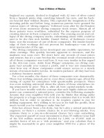
I’ve previously summarized the returns and risks of the major U.S.
stock and bond classes over the twentieth century in Table 1-1. In
Figure 1-19, I’ve plotted these data.
Figure 1-19 showsaclear-cut relationship betweenr
isk and return.

Some may object to the magnitudeof the risksI’veshown for stocks.
But as the recentperformance in emerging markets and tech invest-
ing show, losses in excess of 50% are not unheard of.If you
are not
prepared to accept riskinpursuitof high returns, you are doomed to
fail.
38 The Four Pillars of Investing
Figure 1-19. Risk and return summary. (Source: Kenneth French and Jeremy Siegel.)
CHAPTER 1 SUMMARY
1.The history of the stock and bond markets shows that risk and
reward are inextricably intertwined. Do not expect high returns
without high risk. Do not expect safety without correspondingly
low returns. Further, when the political and economic outlook is
the brightest, returns are the lowest. And it is when things look
the darkest that returns are the highest.
2.
The longer a risky asset is held, the less the chance of a loss.
3. Be especially wary of data demonstrating the superior long-term
performance of U.S. stocks. For most of its history, the U.S. was
a very risky place to invest, and its high investment returns reflect
that. Now that the U.S. seems to be more of a “sure thing,” prices
have risen, and future investment returns will necessarily be
lower.
No Guts, No Glory 39
This page intentionally left blank
The New World Order,
circa 1913
The tragic events in New York, Washington, DC, and
Pennsylvania in the fall of 2001 served to underscore the rela-
tionship between return and risk. Prior to the bombings, most

investors felt that the world had become progressively less risky.
This resulted in a dramatic rise in stock prices. When this illu-
sion was shattered, prices reacted equally dramatically.
This is not a new story. There is no better illustration of the
dangers of living and investing in an apparently stable and pros-
perous era than this passage from Keynes’s The Economic
Consequences of the Peace, which chronicles life in Europe just
before the lights went out for almost two generations:
The inhabitant of London could order by telephone, sipping
his morning tea in bed, the various products of the whole
earth, in such quantity as he might see fit, and reasonably
expect their early delivery upon his doorstep; he could at
the same moment and by the same means adventure his
wealth in the natural resources and new enterprises of any
quarter of the world, and share, without exertion or even
trouble, in their prospective fruits and advantages; or he
could decide, to couple the security of his fortunes with the
good faith of the townspeople of any substantial munici-
pality in any continent that fancy or information might rec-
ommend. He could secure forthwith, if he wished it, cheap
and comfortable means of transit to any country or climate
without passport or other formality, could dispatch his ser-
vant to the neighboring office of a bank for such supply of
the precious metals as might seem convenient, and could
then proceed abroad to foreign quarters, without knowl-
edge of their religion, language, or customs, bearing coined
wealth upon his person, and would consider himself great-
ly aggrieved and much surprised at the least interference.
But, most important of all, he regarded this state of affairs
as normal, certain, and permanent, except in the direction

of further improvement, and any deviation from it as aber-
rant, scandalous, and avoidable. The projects and politics of
militarism and imperialism, of racial and cultural rivalries, of
monopolies, restrictions, and exclusion, which were to play
the serpent to this paradise, were little more than the
amusements of his daily newspaper, and appeared to exer-
cise almost no influence at all on the ordinary course of
social and economic life, the internationalization of which
was nearly complete in practice.
This page intentionally left blank
2
Measuring the Beast
Capital value is income capitalized, and nothing else.
Irving Fisher
43
In the history of modern investing, one economist towers above all
others in influence on the way we examine stocks and bonds. His
name was Irving Fisher: distinguished professor of economics at Yale,
advisor to presidents, famous popular financial commentator, and,
most importantly, author of the seminal treatise on investment value,
The Theory of Interest. And it was Fisher, who, a century ago, first
attempted to scientifically answer the question, “What is a thing
worth?” His career was dazzling, and his precepts are still widely stud-
ied today, more than seven decades after the book was written.
Fisher’s story is a caution to all great men, because, in spite of his
long list of staggering accomplishments, he will be forever remem-
bered for one notorious gaffe. Just before the October 1929 stock mar-
ket crash, he declared, “Stock prices have reached what looks like a
permanently high plateau.” Weeks before the start of a bear market
that would eventually result in a near 90% decline, the world’s most

famous economist declared that stocks were a safe investment.
The historical returns we studied in the last chapter are invaluable,
but these data can, at times, be misleading. The prudent investor
requires a more accurate estimate of future returns for stocks and
bonds than simply looking at the past. In this chapter, we’re going to
explore Fisher’s great gift to finance—the so-called “discounted divi-
dend model” (referred to from now on as the DDM), which allows the
investor to easily estimate the expected returns of stocks and bonds
with far more accuracy than the study of historical returns.
1
1
Many credit John Burr Williams, in his 1938 classic, The Theory of Investment Value,
with the DDM, and, indeed, he fleshed out its mathematics in much greater detail than
Fisher. But The Theory of Interest, published eight years earlier, clearly lays out the
principles of the DDM with sparkling, and at times, entertaining clarity.
Bluntly stated, an understanding of the DDM is what separates the
amateur investor from the professional; most often, small investors
haven’t the foggiest notion of how to estimate a reasonable share price
for the companies they are buying.
You may find this chapter the most difficult in the book; the con-
cepts we will explore are not intuitively obvious, and, in a few spots,
you will have to put the book down and think. But if you can under-
stand the chapter’s central point—that the value of a stock or a bond
is simply the present value of its future income stream—then you will
have a better grasp of the investment process than most professionals.
As we’ve seen, the British enjoy a nearly millennial head start on us
in the capital markets. This has allowed them to embed some bits of
financial wisdom into their culture that we have yet to absorb. Ask an
Englishman how wealthy someone is, and you’re likely to hear a
response like, “He’s worth 20,000 per year.”

This sort of answer usually confuses us less sophisticated Yanks, but
it’s an estimable response, because it says something profound about
wealth: it does not consist of inert assets but, instead, a stream of
income. In other words, if you own an orchard, its value is defined not
by its trees and land but, rather, by the income it produces. The worth
of an apartment house is not what it will fetch in the market, but the
value of its future cash flow. What about your own house? Its value is
the shelter and pleasure it provides you over the years.
The DDM, by the way, is the ultimate answer to the age-old ques-
tion of how to separate speculation from investment. The acquisition
of a rare coin or fine painting for purely financial purposes is clearly
a speculation: these assets produce no income, and your return is
dependent on someone else paying yet a higher price for them later.
(This is known as the “greater fool” theory of investing. When you pur-
chase a rapidly appreciating asset with little intrinsic value, you are
dependent on someone more foolish than you to take it off your hands
at a higher price.) There is nothing wrong with purchasing any of
these things for the future pleasure they may provide, of course, but
this is not the same thing as a financial investment.
Onlyani
ncome-producing possession, such as a stock, bond,or
working piece ofreal estate isatrue investment. Theskeptic will point
out that many
stocks do not havecurrentearningsor produce divi-
dends. True enough, but any stock price abovezero reflects the fact that
at least some investorsconsiderit possiblethat the stock will regain its
earningsand produce dividends in the future,
evenifonly from thesale
ofits assets. And,asBen Graham pointed out decades ago, a stock pur-
chasedwith the hope that its price will soonrise independentofits div-

idend-producing ability isalso a speculation, not
an investment.
44 The Four Pillars of Investing
And lest I unnecessarily offend art lovers, it should be pointed out
that even an old master, bought from the artist for $100 and sold 350
years later for $10,000,000, has returned only 3.34% per year. Ideally,
a fine painting, like a house, is neither a speculation nor an invest-
ment; it is a purchase. Its value consists solely of the pleasure and util-
ity it provides now and in the future. The dividend the painting pro-
vides is of the non-financial variety.
How, then, do we define a stock’s stream of income? Next, how do
we determine its actual worth? This is a tricky problem, which we’ll
tackle in steps. In the next several pages, we’ll uncover how the stock
market is properly valued and how future stock market returns are esti-
mated. These pages may prove difficult. I recommend that you slow
your reading down a bit at this juncture, making sure you have care-
fully read each sentence before proceeding to the next.
One of Fisher’s favorite investment paradigms was a gold or lead
mine that began with a maximum yield in year one, then dwindled to
nothing in 10 years:
Now that we’ve defined the incomes
treamintheabovetable, howdo
we value it? At first glance, it
appearsthat the mine’s worthissimplythe
sum of the income for all ten years—in this case, $11,000. But there’sa
hitch.Humanbeingsprefer presentconsumption to futurec
onsumption.
That is, a dollar ofincome next year is worthless to us than a dollar today,
and a dollarinthirty years, a great dealless than a dollar today. Thus, the
value offuture income must be reduced to reflect its

true present value.
Theamountof this reductionmust take into account four things:
• The number of years you have to wait: The further in the future
you receive income, the less it is worth to you now.
• The rate of inflation: The higher the rate of inflation, the less
value in terms of real spending power you can expect to receive
in the future.
Year Income
1 $2,000
2$1,800
3$1,600
4$1,400
5$1,200
6$1,000
7 $800
8 $600
9 $400
10 $200
Total $11,000
Measuring the Beast 45
• The “impatience” of society forfutureconsumption:The more
society preferspresenttofutureconsumption,the higher are inter-
est rates, and the less future income is worth today. (The
second
and third factorscanbecombinedinto the “realrate ofinterest.”)
• Risk itself: The greater the risk that you might not receive the
income at all, the less its present value.
The simplest way to look at the problem is to imagine waiting in
line to board a plane for a week in Paris. You’ve been working hard
at your job in downtown Cleveland, and you can almost smell the

crêpes on Rue Saint Germain. But wait! Just as you get to the head of
the line, the ticket agent swipes your boarding pass and says, “Sorry
sir, but Hillary Clinton has just arrived, and she needs your seat.”
(You’re flying first class, of course.) “It’s the last one, and the Secret
Service agent demands I give it to her. Don’t worry though, because I
can offer you another trip in ten years.”
What a raw deal! A week in Paris in ten years is not worth nearly as
much to you as a trip right now. You balk. Finally, “I’m sorry, but
you’ll have to make it five weeks in Paris a decade from now to make
it worth my while.” With a sigh of defeat, the agent accepts.
What you have just done is what financial economists call “dis-
counting to the present.” That is, you have decided that a week in
Paris in ten years is worth a good deal less to you than a week there
right now; you have lowered the value of the future weeks in Paris to
account for the fact that you will not be enjoying them for another
decade. To wit, you have decided that five weeks in ten years is worth
as much as just one week today. In the process of doing so, you have
determined that your week-in-Paris discount interest rate is 17.5% per
year; 17.5% is the rate at which one week grows to five weeks over
ten years.
Here is wherethings starttoget a bitsticky, because the discount
rate (referred to fromnow on as the DR) and thepresent value are
inversely related:the higher the DR,
the lower thepresent value. This
isthesameaswith consolsand prestiti, whose values are inversely
related to interest rates. For example, if you decidethat a weekinParis
nowis worth ten weeksadecade fromnow,that implies
a much high-
erDRof 25.9%. This isthesame as saying that thepresent value of a
weekinParis in a decade has cheapened. Again,an increase in the DR

meansthat thepresent value
of a future itemhas decreased; if the value
of one weekinParis nowhas increasedfrom fivetotenweeks in Paris
in the future, then the value of those future weeks has just fallen.
Fisher’s genius was in describing the factors that affect the DR, or
simply, the “interest rate,” as he called it. For example, a starving man
46 The Four Pillars of Investing
would be willing to pay much less for a delayed meal than a well-fed
person. In other words, a hungry person’s DR for food is very high
since he has a more immediate need for it than someone who is well
nourished. Fisher, in fact, uses the words “impatience” and “interest
rate” interchangeably; the wastrel has a higher interest rate (DR) than
the tightwad.
Another of Fisher’s observations was that societies characterized by
highly durable goods have lower interest rates than those that are not.
Where the houses are made of bricks and stone, interest rates are low.
Where the houses are made of mud and straw, rates are high.
Fisher found that, by far, the single most important factor affecting
the DR is risk. The one week/five week Paris trip relationship dis-
cussed above assumed that the airline and travel agent were well-
established and likely to still be in business in ten years when you
return for your vacation. But what if you weren’t so sure that they
would be there for you in a decade? You would, of course, demand a
longer vacation in 10 years—say 10 weeks, instead of five. In which
case, you’ve arrived at the 25.9% DR we mentioned previously. In
other words, the riskier the payoff, the higher the return you would
demand.
Let’s now return to our mine. We have to decide on a discount fac-
tor to apply in each successive year to its income. But before I tell you
just how to estimate the DR, let’s see what a given DR means. Say that

we decide on an 8% DR. The table below is the same one we saw a
few pages ago, but now we’ve added two more columns. The column
labeled “Discount Factor” is the amount we must reduce the dividend
by in a given future year to compute its value in the present day; the
first year’s income must be divided by 1.08, the second year’s by 1.08
ϫ 1.08, and so on. The last column, labeled “Discounted Income,” is
the resultant present value:
Year Income Discount FactorDiscounted Income
1 $2,000 1.0800 $1,852
2$1,800 1.1664 $1,543
3$1,600 1.2597 $1,270
4$1,400 1.3605 $1,029
5$1,200 1.4693$817
6$1,000 1.5869 $630
7 $800 1.7138 $467
8 $600 1.8509 $324
9 $400 1.9990
$200
10 $200 2.1589 $93
Total $8,225
Measuring the Beast 47
For example, look at year 8. In this year, the mine earns $600 but,
just like your delayed trip to Paris, this future payment of $600 is not
worth $600 to you right now. To obtain the current value of this future
$600, you must divide it by 1.8509 (1.08 multiplied by itself seven
times), to yield a value of $324. This is the present value of $600 for
which we must wait eight years at an 8% DR. The total present value
of the mine—in effect, its “true value”—is the sum of all of the future
dividends, discounted to the present. This is the sum at the bottom of
the table: $8,225.

The next step is to apply this method to stocks. The primary job of
the security analyst is to predict the dividend flow of a company so
that it may be discounted to obtain the “fair value” of its stock. If the
market price is below the calculated fair value, it is bought. If the mar-
ket price is above the calculated fair value, it is sold. This is no easy
task. (In fact, as we’ll find out in Chapter 4, it is an impossible task.)
Not infrequently, promising companies with large expected future div-
idend streams stumble and fall; nearly as often, companies given up
for dead recover and provide shareholders with prodigious amounts
of future income.
On the other hand, when you examine an entire market, consisting
of hundreds or thousands of companies, these unexpected events
average out. For this reason, the income stream of the market as a
whole is a much more reliable calculation.
But at first, even this seems a hopeless task. Because the stock mar-
ket is expected to produce dividends forever, you have to predict the
future income stream for an infinite number of future years, discount
the dividends for each year to the present, then add them all up. But
with a few mathematical tricks, this nut is easily cracked.
A Stream of Future Dividends, Forever and Ever, Amen
To paraphrase the famous Chinese proverb, even a journey of a thou-
sand miles must begin with a single step. Here’s our first one. At the
end of 2001, the Dow Jones Industrial Average was selling at around
9,000 and yielded 1.55% of that, or about $140 per year in dividends.
Further, over the long haul, the Dow’s dividends grow at about 5% per
year. So in 2002, there should be about $147 of dividends; in 2031,
$605. Now take a look at Table 2-1. In the second column, under
“Nominal Dividends” (“nominal” refers to the actual dollar amount,
not adjusted for inflation), I’ve tabulated the actual dividend for each
future year; I’ve also plotted this rise in dividends in Figure 2-1.

We’ve just taken the first step in valuing the market: we’ve defined
its future stream of dividends. Next, we must discount the actual divi-
48 The Four Pillars of Investing
Measuring the Beast 49
Table 2-1. Dow Jones Industrial Average Projected and Discounted Dividends
8% 8% 15% 15%
Nominal Discount Discount Discount Discount
Year Dividends FactorValue FactorValue
2001 $140.00 1.00 $140.00 1.00 $140.00
2002 $147.00 1.08 $136.11 1.15 $127.83
2003 $154.35 1.17 $132.33 1.32 $116.71
2004 $162.071.26 $128.65 1.52 $106.56
2005 $170.17 1.36 $125.08 1.75 $97.30
2006 $178.681.47 $121.61 2.01 $88.84
2007 $187.611.59 $118.23 2.31 $81.11
2008 $196.99 1.71 $114.94 2.66 $74.06
2009 $206.84 1.85 $111.75 3.06 $67.62
2010$
217.19 2.00 $108.65 3.52 $61.74
2011 $228.05 2.16 $105.63 4.05 $56.37
2012 $239.45 2.33 $102.69 4.65 $51.47
2013 $251.42 2.52 $99.84 5.35 $46.99
2014 $263.99 2.72 $97.07 6.15 $42.91
2015$277.19 2.94 $94.37 7.08 $39.17
2016$291.05 3.17 $91.75 8.14 $35.77
2017 $305.60 3.43 $89.20 9.36 $32.66
2018 $320.88 3.70 $86.72 10.76 $29.82
2019 $336.93 4.00 $84.32 12.38 $27.23
2020 $353.77 4.32 $81.97 14.23 $24.86
2021 $371.46 4.66 $79.70 16.37 $22.70

2022 $390.03 5.03 $77.48 18.82 $20.72
2023 $409.54 5.44 $75.33 21.64 $18.92
2024 $430.01 5.87 $73.24 24.89 $17.28
2025 $451.51 6.34 $71.20 28.63 $15.77
2026 $474.09 6.85 $69.23 32.92 $14.40
2027 $497.79 7.40 $67.30 37.86 $13.15
2028 $522.687.99 $65.43 43.54 $12.01
2029 $548.82 8.63 $63.62 50.07 $10.96
2030 $576.26 9.32 $61.85 57.58 $10.01
2031 $605.0710.06 $60.13 66.21 $9.14
2032 $635.33 10.87 $58.46 76.14 $8.34
2033 $667.0911.74 $56.84 87.57 $7.62
2034 $700.45 12.68 $55.26 100.70 $6.96
2035 $735.4713.69 $53.72 115.80 $6.35
2036 $772.24 14.79 $52.23 133.18 $5.80
2037 $810.85 15.97 $50.78 153.15 $5.29
2038 $851.40 17.25 $49.37 176.12 $4.83
2039 $893.97 18.63 $48.00 202.54 $4.41
2040 $938.67 20.12 $46.66 232.92 $4.03
2041 $985.60 21.72 $45.37 267.86 $3.68
2042 $1,034.88 23.46 $44.11 308.04 $3.36
dend in each future year to the present. To do this, we divide the div-
idend in each future year by the appropriate discount factor, similar to
our calculation for the mine. How do we decide on a DR for the entire
stock market? Similar to our hypothetically discounted future meal, the
50 The Four Pillars of Investing
Table 2-1. (Continued)
8% 8% 15% 15%
Nominal Discount Discount Discount Discount
Year Dividends FactorValue FactorValue

2043 $1,086.62 25.34 $42.88 354.25 $3.07
2044 $1,140.9527.37 $41.69 407.39 $2.80
2045 $1,198.00 29.56 $40.53 468.50 $2.56
2046 $1,257.9031.92 $39.41 538.77 $2.33
2047 $1,320.80 34.47 $38.31 619.58 $2.13
2048 $1,386.8437.23 $37.25 712.52 $1.95
2049 $1,456.18 40.21 $36.21 819.40 $1.78
2050
$1,528.99 43.43 $35.21 942.31 $1.62
Etc. Etc. Etc. Etc. Etc. Etc.
Sum of Discounted Dividends
in All Years $4,667.67 $1,400.00
Figure 2-1. Dow dividend value.
DR of the Dow is simply the rate of return we expect from it, taking its
risk into consideration.
Let’s say that we expect an 8% return from stocks. So just like our
mine, the market’s DR, by definition, is thus 8%. As we’ve already
determined, the Dow’s dividend 30 years from now should be about
$605. Similar to our mine, to get the present value of those dividends
we have to divide that amount by 1.08 for each year in the future. To
obtain the present value of the Dow dividend 30 years from now, in
2031, you have to divide $605 by 10.06 (1.083
30
, that is, 1.08 multiplied
by itself 29 times). Dividing the $605 dividend in 2031 by 10.06 yields
a present value of $60. If we perceive that economic, political, or mar-
ket risk has increased, we may decide that the DR should be higher;
if we are really frightened about the state of the economy, the nation,
or the world, we will decide that 15% is appropriate. In that case, the
present value of the year 2031’s $605 dividend is reduced even further,

to just $9.
Take another look at Table 2-1. Again, the second column in this
table displays the nominal expected dividends, which rise at a 5%
annual rate in each future year. The third column is the discount fac-
tor at 8% for each year. The fourth column is the value of the dividend
in that year, discounted to the present (this is calculated by dividing
the actual dividend in the second column by the discount factor in the
third). As with prestiti and consols, when the DR rises, prices fall;
when the DR falls, prices rise.
I’ve also plotted these numbers in Figure 2-2. The top curve—the
same curve plotted in Figure 2-1—represents the actual, or “nominal,”
dividends received in each future year. To reiterate, the top curve rep-
resents the actual dividend stream of the Dow received by sharehold-
ers before its value has been adjusted down to its present value. The
bottom curves are the present value of the Dow’s income stream,
obtained by discounting the nominal dividends at rates of 8% and 15%.
Notice how at the higher discount rate, the discounted value of the
dividends decays nearly to zero after a few decades; such is the cor-
rosive effect of high DRs, caused by high risk or high inflation, on
stock values.
Better Living Through Mathematics
Now we need only perform one more step. To obtain the “true value”
of the Dow, you have to add together all of the discounted dividends
for each year (excluding the first, because it has already been paid).
For example at a DR of 8%, you would add up all of the numbers
(except the first) in the fourth column, the one labeled “8% Discount
Measuring the Beast 51
Value.” Does this seem like a hopelessly difficult task? It is, if you are
doing the computation by what mathematicians call the “brute force”
method, i.e., trying to add the infinite column of numbers in column

four.
Fortunately, mathematicians can help us out of this pickle with a
simple formula that calculates the sum of all of the desired values in
column four. Here it is:
Market Value ϭ Present Dividend/(DR Ϫ Dividend Growth Rate)
Using our assumption of a $140 present dividend, an 8% DR, and
5% earnings growth, we get:
Market Value ϭ $140/(0.08Ϫ0.05) ϭ $140/0.03 ϭ $4,667
(Finance types always do their calculations with decimals; 8%
becomes 0.08 in the formula.)
Oops. This formulation suggests that the Dow, currently priced at
around 10,000, is about 100% overvalued compared to the 4,667 value
we just computed using the rosy 8% DR Ϫ return scenario.
And if things get really rough, investors may decide they require a
15% DR to invest in stocks (as they did in the early 1980s, when
52 The Four Pillars of Investing
Figure 2-2. Discounted Dow dividend value.
Treasury bonds yielded almost 16%). I’ve shown the relevant figures
for a 15% DR in the last two columns of Table 2-1. The simplified cal-
culation looks like this:
Market Value ϭ $140/(0.15 Ϫ 0.05) ϭ $140/0.10 ϭ $1,400
It is unlikely (but not impossible) that the Dow will drop as far as
1,400 at any point in the future, but recall that at least twice in this cen-
tury U.S. investors indeed did demand a 15% DR.
This kind of calculation is enormously sensitive to the DR and divi-
dend growth rate. For example, raise earnings growth to 6% and lower
the DR to 7%, and you come up with a market value of 14,000. Some
of you may be aware of the controversy surrounding a book by James
Glassman and Kevin Hassett, provocatively titled Dow 36,000, in
which they arrive at the title’s number by fiddling with the above equa-

tion in the manner we’ve described.
In fact, using entirely reasonable assumptions, you can make the
Dow’s discounted market value almost anything you want it to be. To
show how the DR affects the “fair value” of the Dow via this tech-
nique, I’ve plotted the Dow’s “fair value” from the DDM versus the DR
in Figure 2-3.
Rescued by the Gordon Equation
Why have we spent so much time and effort on the DDM when it turns
out that it cannot be used to accurately price the stock market? For
Measuring the Beast 53
Figure 2-3. Dow fair value versus discount rate.
three reasons. First and foremost, because it provides an intuitive way
to think about the value of a security. A stock or bond is not an
abstract piece of paper that has a randomly fluctuating value; it is a
claim on real future income and assets.
Second, it enables us to test the growth and return assumptions of
a stock or of the entire market. At the height of the tech madness in
April 2000, the entire Nasdaq market sold at approximately 100 times
earnings. Applying the DDM to it revealed that this implied either a
ridiculously high earnings growth rate or a low expected return. The
latter seemed far more plausible to serious observers, and unfortu-
nately, this is eventually what happened.
Third, and most important, the real beauty of the above formulas is
that they can be rearranged to calculate the market’s expected return,
producing an equation that is at once stunningly simple and powerful:
DR (Market Return) ϭ Dividend Yield ϩ Dividend Growth
This formula, which is known as the “Gordon Equation,” provides
an accurate way to predict long-term stock market returns. For exam-
ple, during the twentieth century, the average dividend yield was
about 4.5%, and the compounded rate of dividend growth was also

about 4.5%. Add the two together and you get 9.0%. The actual return
was 9.89%—not too shabby. The approximately 1% difference was due
to the fact that stocks had become considerably more expensive (that
is, the dividend yield had fallen) during the period.
The Gordon Equation also has an elegant intuitive beauty. If the
stock market is simply viewed as a source of dividends, then its price
should rise in proportion to those dividends. So if its dividends
increase at 4.5% per year, then over the very long term its price should
also increase by 4.5% per year. In addition to the price increase, you
also receive the actual dividend each year: the annualized total return
comes from the combination of the annualized price increase (which
is roughly the same as the annualized dividend growth) and the aver-
age dividend yield.
The Gordon Equation is as close to being a physical law, like grav-
ity or planetary motion, as we will ever encounter in finance. There
are those who say that dividends are quaint and outmoded; in the
modern era, return comes from capital gains. Anyone who really
believes that might as well be wearing a sandwich board on which is
written in large red letters, “I haven’t the foggiest notion what I’m talk-
ing about.”
It is, of course, true that a company never has to pay out a dividend
in order to provide capital gains. But even if all of the companies in
the U.S. stopped paying out dividends (which they have just about
54 The Four Pillars of Investing
done), in the long term their return would be roughly the same as their
aggregate earnings growth. Thus, in a world without dividends, com-
pany earnings must grow at an average rate of 10% per year in order
to provide the historical 10% long-term return of stocks. And, as we’ll
soon see, the long-term average rate of corporate earnings and divi-
dend growth is only 5%. Worse, when adjusted for inflation, it has not

changed in the past century.
Never forget that in the long run, it is corporate earnings growth that
produces stock price increases. If, over the very long term, the annu-
alized earnings growth is about 5%, then the annualized stock price
increase must be very close to this number.
One exception to this is the case of companies that are buying back
their shares. A company that has grown its earnings by 5% per year
and annually buys back 5% of its outstanding shares will appreciate by
10% per year, in the long term. The opposite is true of companies that
issue new stock. Averaged over the whole U.S. market, these two fac-
tors tend to cancel each other out.
The discounted dividend model is a powerful way of understanding
stock and bond behavior. As we’ve seen, it isn’t of much use in accu-
rately predicting the fair value of the market, let alone a stock.
Princeton economist Burton Malkiel famously stated that “God
Almighty himself does not know the proper price-earnings multiple for
a common stock.” In other words, it is impossible to know the intrin-
sic value of a stock or the market. But the DDM is useful in more sub-
tle, powerful ways. First, it can be used in reverse. That is, instead of
entering the estimated dividend growth and DR and getting the price,
we can derive these two values from the price of the market or for a
given stock. We’ve already seen that in 1999, for example, applying
the DDM in this manner would have told you that highly unrealistic
growth expectations were embedded in the prices of tech stocks.
And,of course,
the DDM gives
us theGordonEquation, which
allowsustoestimate stockreturns. This raises animportantpoint.
Wall Street and the mediaareconstantlyobsessedwith the question
ofwhether the market isovervalued or undervalued(and

by implica-
tion, whetherit is headed up ordown). As we’ve just seen,this is
essentially impossibletodetermine. But in theprocess, we’ve just
acquired a muchmore valuable bitofknowledge: the long-term
expected return of the market. Think about it, whichwould you rather
know:the market return
for the next six months, orfor the next 30
years? I don’t know about you, but I’d muchratherk
now the latter.
And, within a reasonable margin of error, you can. But you don’tsell
newspapers, magazines, and airtime speculating about 30-year
returns.
Measuring the Beast 55
And what does the Gordon Equation tell us today about future stock
returns? The news, I’m afraid, is not good. Dividend growth still seems
to be about 5%, and the yield, as we’ve already mentioned, is only
1.55%. These two numbers add up to just 6.55%. Even making some
wildly optimistic assumptions—say a 6% to 7% dividend growth rate—
does not get us anywhere near the 10% annualized returns of the past
century.
What about bonds? The expected return of a long-term bond is sim-
ply its “coupon,” that is its interest payments. (For a bond, the second
number in the Gordon Equation, dividend growth, is zero. In almost
all cases, a bond’s interest does not grow.) High-quality corporate
bonds currently yield about 6%. This figure provides a reasonably
accurate estimate of their future returns. If interest rates rise, their
value will fall, but the rate at which the interest is reinvested will rise,
and vice versa. So over a 30-year period, the total bond return cannot
be very far from the 6% coupon.
What we have now is a very different picture from what transpired

in the twentieth century, with its high stock returns and low bond
returns. Going forward, it looks like stock and bond returns should
both be in the 6% range, not the 10% historical reward. Don’t shoot
me, I’m only the messenger.
Viewed from an historical perspective, what has happened is that
stocks have had an incredible run the past few decades. Their prices
have been bid up dramatically, so their future returns will be com-
mensurately lower. The exact opposite has happened to bonds. As
we’ve already seen, bondholders were severely traumatized by the
unprecedented monetary shift in the twentieth century. Their prices
have fallen, so their expected returns have commensurately risen.
On ani
ntellectuallevel, most investors have notroubleunderstand-
ing the notion that high past returns result in high prices, which, in
turn, result in lowerfuture returns. But at thesametime, most investors
find thisalmost impossible
to accept on an emotionallevel. Bysome
strangequirk ofhumannature, financial assets seem to become more
attractiveafter their price has risengreatly. But buying stocksand
bonds is no differentthanbuying tomatoes.
Most folksaresensible
enough to load up when thetomatoes areselling at 40 cents per
pound and to forgothem at three dollars. But stocksare different. If
prices fall drasticallyenough,they becomethe lepersof the financial
world.C
onversely, if prices rise rapidly, everyone wants in on the fun.
Until very recently, there was a great deal of talk about the “new
investment paradigm.” Briefly stated, this doctrine asserts that Fisher
had gotten it all wrong: earnings, dividends, and price no longer mat-
ter. The great companies of the New Economy—Amazon, eToys, and

56 The Four Pillars of Investing
Cisco—were going to dominate the nation’s business scene, and no
price was too high to pay for the certain bonanza these firms would
provide their shareholders.
Of course, we’ve seen this movie before. In 1934, the great invest-
ment theorist Benjamin Graham wrote of the pre-1929 stock bubble:
Instead of judging the market price by established standards of
value, the new era based its standards of value upon the mar-
ket price. Hence, all upper limits disappeared, not only upon
the price at which a stock could sell, but even upon the price
at which it would deserve to sell. This fantastic reasoning actu-
ally led to the purchase for investment at $100 per share of
common stocks earning $2.50 per share. The identical reason-
ing would support the purchase of these same shares at $200,
at $1,000, or at any conceivable price.
Even the most casual investor will see the parallels of Graham’s
world with the recent tech/Internet bubble. Graham’s $100 stock sold
at 40 times its $2.50 earnings. At the height of the 2000 bubble, most
of the big-name tech favorites, like Cisco, EMC, and Yahoo! sold at
much more than 100 times earnings. And, of course, almost all of the
dot-coms went bankrupt without ever having had a cent of earnings.
At the end of the day, the Fisher DDM method of discounting inter-
est streams is the only proper way to estimate the value of stocks and
bonds. Future long-term returns are quite accurately predicted by the
Gordon Equation. As I’ve already said, these are essentially the laws
of gravity and planetary motion of the financial markets. But it seems
that once every 30 years or so, investors tire of valuing stocks by these
old-fashioned techniques and engage in orgies of unthinking specula-
tion. Invariably, Fisher and Graham’s lesson—not to overpay for
stocks—is re-learned in excruciating slow motion in the years follow-

ing the inevitable market crash.
The rubis,
theGordonEquationis useful only in the long term—
ittellsusnothing about day-to-day, or even year-to-year, returns. And
eveninthe very long term, it is not
perfect. As we’vealready seen
above, over the course of thetwentieth century, it was off byabout
1%of annualizedreturn.This 1% difference canbe attributed to the
change in the dividend
rate, whichdecreasedfrom 4.5% to 1.4%
between1900 and 2000. In otherwords, stocks, whichin1900 sold
for 22 times their dividends, now sell for70times their dividends. The
ratioof price to dividends—22 in 1900, 70 in 2000—iscalled the “div-
idend multiple.”(This issimplythe inverse
of the dividend yield:
1/.045 ϭ 22, and 1/.014 ϭ 70.) This ratio isthe number ofdollars you
must pay to get one dollar of dividends. It issimilar to the more famil-
Measuring the Beast 57
iar“PEmultiple”:price dividedbyearnings. ThePEmultiple isthe
most popularmeasureofhow“expensive” the stockmarket is.
The Gordon Equation does not account for changes in the dividend
or PE multiple. The tripling of the dividend multiple between 1900 and
2000 accounts for most of the approximately 1% difference between
the 9% predicted by the Gordon Equation and the 9.89% actual return.
(Compounding 0.89% over a century produces close to a tripling of the
stock market’s value.) Stating that there was a “tripling of the dividend
multiple” is just another way of saying that an enthusiastic investing
public has driven up stock prices relative to earnings and dividends by
a factor of three.
Over relatively short periods of time—less than a few decades—this

change in the dividend or PE multiple accounts for most of the stock
market’s return, and over periods of less than a few years, almost 100%
of it. John Bogle, founder of the Vanguard Group of mutual funds,
provides us with a very useful way of thinking about this. He calls the
short-term fluctuations in stock prices due to changes in dividend and
PE multiples the “speculative return” of stocks.
On theo
therhand,the long-term increase in stockmarket value is
entirelythe resultof thesum oflong-term dividend growth and dividend
yield calculatedfrom theGordonEquation, what Boglecallsthe “fun-
damentalreturn” of stocks.
In engineering terms, Bogle’s fundamental
return isthesignal—aconstant, reliable occurrence. Bogle’s speculative
return isthe noise—distracting and unpredictable. For example,
on
October19, 1987,the stockmarket fell by 23%. Certainly, on that day—
Black Monday—there were nosignificantchanges in the dividend pay-
ments or dividend growth of common stocks. The market crash of
1987,
and the run up which precededit, werepurely speculativeevents.
The key point, which we’ll return to again and again, is that the fun-
damental return of the stock market—the sum of dividends and divi-
dend growth—is somewhat predictable, but only in the very long
term. The short-term return of the market is purely speculative and
cannot be predicted. Not by anyone. Not the panelists on Wall Street
Week, not the “market strategists” at the biggest investment houses, not
the newsletter writers, and certainly not your stockbroker.
Perhaps
somewhere in a dark secret corner ofWall Street,
there isone

personwho knows just wherethe market is going tomorrow. But if she
exists, she would of course not tell a soulforfear of tipping off the mar-
ket and damaging theenormous profits
that aretobe herson the mor-
row. (Or,asfinancial economist Rex Sinquefield replies with astraight
face when asked about the direction of the stockmarket, “I knowwhere
the market’s headed,Ijust don’t wantt
osharethat with anyone.”)
A superb metaphor for the long-term/short-term dichotomy in stock
58 The Four Pillars of Investing
returns comes from Ralph Wanger, the witty and incisive principal of
the Acorn Funds. He likens the market to an excitable dog on a very
long leash in New York City, darting randomly in every direction. The
dog’s owner is walking from Columbus Circle, through Central Park,
to the Metropolitan Museum. At any one moment, there is no predict-
ing which way the pooch will lurch. But in the long run, you know
he’s heading northeast at an average speed of three miles per hour.
What is astonishing is that almost all of the market players, big and
small, seem to have their eye on the dog, and not the owner.
As we’ve already mentioned, the Gordon Equation is not good news
for future equity returns. Is there any way out of this gloomy scenario?
Yes. There are three possible scenarios in which equity returns could
be higher than the predicted 6.4%:
•
Dividend growth could accelerate. Companies usually only pay
part of their dividends out as earnings. At the present time, the
market sells at about 25 times its annual earnings. Another way
of saying this is that the “earnings yield” of the market is 4%
(1/25). So, if these companies are paying out 1.4% as dividends,
that leaves 2.6% to pay for growth.

The above figures represent an average of the whole market.
Many companies earn far more or far less than 4% of their market
value, while many, like Microsoft, pay out zero dividends, retain-
ing all their earnings for future growth. It is said that U.S. compa-
nies have experienced dramatic increases in productivity in the
past few decades, and that this will further accelerate earnings
growth beyond the 5% historical figure. This is wishful thinking.
In the first
place, before 1980, companies kept farmorethan
2.6% of their capitalvalue in retained earnings. In the second place,
there is voluminous evidence
that excess corporate cashfrom
“retained earnings”(that is, earnings not paid out to thesharehold-
ers, but insteadreinvestedinthecompany) tendstobe wasted. And
finally, it just isn’t happening.In Figure2-4, I’veplotted the divi-
dendsand earningsof the
stockmarket since 1900 (courtesy of
RobertShiller at Yale). Figure2-4 isanother oneof those confusing
“semilog” graphs. Their major advantage isthat they allow you to
estimate thepercent rate
ofincrease of earningsand dividends
across a wide rangeofvalues. This is not true of standard “arith-
metic” plots. With asemiloggraph,aconstant growthrate produces
aplot that moves up at a fairlyconstantangle, called theslope.
This
is approximately what is seeninFigure2-4.
Those of you with an eagle eye will detect that the slope for
the first 50 years seems to be ever-so-slightly less than for the last
Measuring the Beast 59