Báo cáo toán học: " Order-distributions and the Laplace-domain logarithmic operator" docx
Bạn đang xem bản rút gọn của tài liệu. Xem và tải ngay bản đầy đủ của tài liệu tại đây (525.27 KB, 19 trang )
RESEARC H Open Access
Order-distributions and the Laplace-domain
logarithmic operator
Tom T Hartley
1*
and Carl F Lorenzo
2
* Correspondence:
1
Department of Electrical and
Computer Engineering, University
of Akron, Akron, OH 44325-3904,
USA
Full list of author information is
available at the end of the article
Abstract
This paper develops and exposes the strong relationships that exist between time-
domain order-distributions and the Laplace-domain lo garithmic operator. The paper
presents the fundamental theory of the Laplace-domain logarithmic operator, and
related operators. It is motivated by the appearance of logarithmic operators in a
variety of fractional-order systems and order-distributions. Included is the
development of a system theory for Laplace-domain logarithmic operator systems
which includes time-domain representations, frequency domain representations,
frequency response analysis, time response analysis, and stability theory.
Approximation methods are included.
Keywords: Order-distribution, Laplace transform, Fractional-order systems, Fractional
calculus
Introduction
The area of mathematics known as fractional calculus has been studied for over 300
years [1]. Fra ctional-order systems, or systems described using fractional derivatives
and integrals, have been studied by many in the engineering area [2-9]. Additionally,
very readable discussions, devoted to the mathemat ics of t he subj ect, are presented by
Oldham and Spanier [1], Miller and Ross [10], Oustaloup [11], and Podlubny [12]. It
should be noted that there are a growing number of physical systems whose behavior
can be compactly described using fractional-order system theory. Specific app lications
are viscoelastic materials [13-16], electrochemical processes [17,18], long lines [5],
dielectric polarization [19], colored noise [20], soil mechanics [21], chaos [22], control
systems [23], and optimal control [24]. Conferences in the area are held annually, and
a particularly interesting publication containing many applications and numerical
approximations is Le Mehaute et al. [25].
The concept of an order-distribution is well documented [26-31]. Essentially, an
order-distribution is a parallel connection of fractional-order integrals and derivatives
taken to the infinitesimal limit in delta-order. Order-distributions can arise by design
and construction, or occur naturally. In Bagley [32], a thermo-rheological fluid is dis-
cussed. There it is shown that the order of the rheological fluid is roughly a linear
function of temperature. Thus a spatial temperature distribution inside the material
leads to a related spatial dist ribution of system orders in the rheological fluid, that is,
the position-force dynamic response will be represented by a fractional-order derivative
whose order varies with position or temperature inside the material. In Hartley and
Hartley and Lorenzo Advances in Difference Equations 2011, 2011:59
/>© 2011 Hartley and Lorenzo; licensee Springer. This is an Open Access article distributed under the terms of the Creative Commons
Attribution License ( which permits unrestricted use, distribution, and reproduction in
any medium, provid ed the original work is properly cited.
Lorenzo [33], it is shown that various order-distributions can lead to a variety of trans-
fer functions, many of which contain a ln(s)term,wheres is the Laplace variable.
Some of these result s are reproduced in the tables at the end of this paper. In Adams
et al. [ 34], it is shown that a conjugated-order derivative can lead directly to terms
containing ln(s). In Adams et al. [35], it is also shown that the conjugated derivative is
equivalent to the third generation CRONE control which has been applied extensively
to control a variety of systems [25].
The purpose of this paper is to provide an understanding of the ln(s) operator, the
Laplace-domain logarithmi c operator, and determine what special properties are asso-
ciated with it. The motivation is the frequent occurrence of the ln(s) operator in pro-
blems whose dynamics are expressed as fractional-order systems or order-distributions.
This can be seen in Figure 1 which shows the transf er functions corresponding to sev-
eral order-distributions, taken from Hartley and Lorenzo [33]. This figure demonstrates
that the ln(s) operator appears frequently.
The next section will review the necessary results from fractional calculus and the
theory of order-distributions. It will then be shown that the Laplace-domain logarith-
mic operator arises naturally as an order distributi on, thereby providing a method for
constructi ng a logarithmic operator eith er in the time or frequency domain. It is then
shown that Laplace-domain logarithmic operators can be combined to form systems of
logarithmic operators. Following this is the development of a system theo ry for
Laplace-domain logarithmic operator systems which includes time-domain representa-
tions, frequency domain representations, frequency response analysis, time response
analysis, and stability theory. Fractional-order approximations for logarithmic operators
are then developed using finite differences. The paper concludes with some special
order-distribution applications.
()Xs ()
F
s
1
ln( )
s
1
q
s
2
q
s
3
q
s
4
q
s
n
q
s
()Xs
6
0
() (), 1
q
Fs s dqXs s
f
!
³
Figure 1 High frequency continuum order-distribution realization of the Laplace-domain reciprocal
logarithmic operator.
Hartley and Lorenzo Advances in Difference Equations 2011, 2011:59
/>Page 2 of 19
Order-distributions
In Hartley and Lorenzo [30,33], the theory of order-distributions has been presented. It
is based on the use of fractional-order differentiation and integration. The definition of
the uninitialized qth-order Riemann-Liouville fractional integral is
0
d
−q
t
x(t) ≡
1
(q)
t
0
(t − τ )
q–1
x(τ )dτ , q ≥ 0
(1)
The pth-order fractional derivative is defined as an integer derivative of a fractional
integral
0
d
p
t
x(t) ≡
1
(1 − p)
d
dt
t
0
(t − τ )
−p
x(τ )dτ 0, < p < 1
(2)
If higher deriv atives are desired (p > 1), multiple integer derivatives are taken of the
appropriate fractional integral. The integer derivatives are taken as in the standard cal-
culus. In what follows, it will be important to use the Laplace transform of the frac-
tional integrals and derivatives. This Laplace transform is given in Equation 3, where it
is assumed that any initialization is zero
L
0
d
q
t
x(t)=s
q
X(s)for all q
(3)
By comparing the convolution operators with the Laplace transforms, a fundamen-
tally useful Laplace transform pair is
Lt
q−1
=
(q)
s
q
, q > −1
(4)
Here it can be seen that an operator such as that in Equation 3, can also be written
as a Laplace-domain operator as
F( s )=s
q
X(s).
where for example, f(t) could be force, and x(t) could be displacement. Now if there
exists a collection of these individual fractional-order operators driven by the same
input, then their outputs can be combined
F( s )=k
1
s
q
1
X(s)+k
2
s
q
2
X(s)+k
3
s
q
3
X(s)+k
4
s
q
4
X(s)+··· =
N
n=1
k
n
s
q
n
X(s)
where the k’s are weightings on each fractional integral. Taking the summation to a
continuum limit yields the definition of an order-distribution
⎛
⎝
q
max
0
k(q)s
q
X(s)dq
⎞
⎠
=
⎛
⎝
q
max
0
k(q)s
q
dq
⎞
⎠
X(s)=F(s),
(5)
where q
max
is an upper limit on the differential order and sho uld be finite for the
integral to converge, and k(q) must be such that the integral is convergent. Equation 5
has the uninitialized time domain representation
Hartley and Lorenzo Advances in Difference Equations 2011, 2011:59
/>Page 3 of 19
q max
0
k(q)
0
d
q
t
x(t)dq = f (t)
(6)
Order-distributions can also be defined using integral operators instead of differential
operators as
X(s)=
⎛
⎝
∞
0
k(q)s
−q
F( s ) dq
⎞
⎠
=
⎛
⎝
∞
0
k(q)s
−q
dq
⎞
⎠
F( s ),
(7)
The uninitialized time domain representation of Equation 7 is
∞
0
k(q)
0
d
q
t
f (t)dq = x(t)
(8)
As a further generalization, in Equation 5, the lower limit of integration can be
extended below zero to give
⎛
⎝
q max
0
k(q)s
q
d(s)dq
⎞
⎠
X(s)=F(s)
(9)
where again, k(q) must be chosen such that the integral converges. Even more gener-
ally, an order distribution can be written as
⎛
⎝
b
a
k(q)s
–q
dq
⎞
⎠
X(s)=−
⎛
⎝
−a
−b
k(−q)s
q
dq
⎞
⎠
X(s)=F(s), a < b.
(10)
The Laplace-domain logarithmic operator
The logarithmic operator can now be defined using the order-distribution conce pt. In
Equation 10, let k(q) be unity over the region of integration, a = 0, and b equal to infi-
nity. Then the order-distribution is
F( s )=
⎛
⎝
∞
0
s
−q
dq
⎞
⎠
X(s)=−
⎛
⎝
0
−∞
s
q
dq
⎞
⎠
X(s).
(11)
Evaluating the first integral on the left gives
F( s )=
∞
0
s
−q
dq
X(s)=
∞
0
e
−qln(s)
dq
X(s)=
e
−qln(s)
-ln(s)
X(s)
∞
0
,
|
s
|
> 1,
=
e
−∞ln(s)
-ln(s)
−
e
−0ln(s)
-ln(s)
X(s),
|
s
|
> l
.
Thus
F( s )=
⎛
⎝
∞
0
s
−q
dq
⎞
⎠
X(s)=
1
ln(s)
X(s), | s |> 1
(12)
Hartley and Lorenzo Advances in Difference Equations 2011, 2011:59
/>Page 4 of 19
With the constraint that |s| > 1 for the integral to converge, it is seen that this
order-distribution is an exact representation of the Laplace domain logarithmic opera-
tor at high frequencies, ω > 1, or small time. From Equation 12, it can be seen that the
reciprocal Laplace-domain logarithmic operator can be represented by the sum of all
fractional-order integrals at high frequencies, ω > 1. This can be visualized as shown
in Figure 2.
At high frequencies, ω > 1, the time-domain operator corresponding to Equation 12
is
f (t)=
∞
0
t
0
(t − τ )
q−1
(q)
x(τ )dτ dq,
(13)
so that
1
ln(s)
X(s) ⇔
∞
0
t
0
(t − τ )
q−1
(q)
x(τ )dτ dq.
These results are verified by the Laplace transform pair given in Roberts and Kauf-
man
1
ln(s)
⇔
∞
0
t
q−1
(q)
dq,
(14)
which is obtained from Equation 13 by letting x(t)=δ(t), a unit impulse. It is impor-
tant to note that the time domain function on t he right-hand side of Equation 14 is
known as a Volterra function, and is defined for all positive time, not just at high fre-
quencies (small time) [36].
()Xs
1
q
s
2
q
s
3
q
s
6
0
() (), 1
q
Fs sdqXs s
f
³
()Xs ()
F
s
1
ln( )
s
4
q
s
n
q
s
Figure 2 Low frequency continuum order-distribution realization of the Laplace-domain reciprocal
logarithmic operator.
Hartley and Lorenzo Advances in Difference Equations 2011, 2011:59
/>Page 5 of 19
Referring back to Equation 10, again let k(q) be unity over the region of integration,
a = negative infinity, and b=0. Then the order-distribution is
F( s )=
⎛
⎝
0
−∞
s
−q
dq
⎞
⎠
X(s)= −
⎛
⎝
+∞
0
s
q
dq
⎞
⎠
X(s).
(15)
Evaluating the integral on the right gives
F( s )=−
⎛
⎝
∞
0
s
q
dq
⎞
⎠
X(s)=−
⎛
⎝
∞
0
e
qln(s)
dq
⎞
⎠
X(s)=−
e
qln(s)
ln(s)
X(s)
∞
0
,
|
s
|
< 1,
= −
e
∞ln(s)
ln(s)
−
e
0ln(s)
ln(s)
X(s),
|
s
|
< l.
Thus,
F( s )=−
⎛
⎝
∞
0
s
q
dq
⎞
⎠
X(s)=
1
ln(s)
X(s), | s |< 1.
(16)
With the constraint that |s| < 1 for the integral convergence, it is seen that this
order-distribution is an exact representation of the Laplace domain logarithmic opera-
tor at l ow frequencies, ω < 1, or large time. From Equation 16, it can be seen that the
reciprocal Laplace-domain logarithmic operator can be represented by the sum of all
fractional-order derivatives at low frequencies (large time). This can be visualized as
shown in Figure 3.
At low frequencies, ω < 1, or large time, the integral over all the fractional deriva-
tivesmustbeusedasinEquation16.Thetime-domain operator corresponding to
Equation 16 is then, with q = p - u,
f (t)=
∞
0
d
p
dt
p
t
0
(t − τ )
u−1
(u)
x(τ )dτ dq, p = 1,2,3, , p > q > p − 1,
(17)
v
/2
T
S
/2
T
S
unstablestripcorrespondsto
rightͲhalfsͲplane
uppervͲplanecorrespondsto
upperleftͲhalfsͲplane
lowervͲplanecorrespondsto
lowerleftͲhalfsͲplane
s
f0s
increasing
s
increasing
s
Figure 3 Stable and unstable regions of the v = ln(s) plane.
Hartley and Lorenzo Advances in Difference Equations 2011, 2011:59
/>Page 6 of 19
so that
1
ln(s)
X(s) ⇔
∞
0
d
p
dt
p
t
0
(t − τ )
u−1
(u)
x(τ )dτ dq, p =1,2,3, , p > q > p−1, | s |< 1.
(18)
Letting the input x(t)=δ(t), a unit impulse, this equation becomes
1
ln(s)
X(s) ⇔
∞
0
d
p
dt
p
(t)
u−1
(u)
dq, p =1,2,3, , p > q > p − 1, | s |< 1.
(19)
Performing the integral yields
1
ln(s)
⇔
∞
0
t
−q−1
(−q)
dq.
(20)
The properties of this integral require further study, although it appears to be con-
vergentforlargetimeduetothegamma function going to infinity when q passes
through an integer and thus driving the integrand to zero there.
Higher powers of the Laplace-domain logarithmic operator
Higher powers of logarithmic operators can be generated using order distributions. In
Equation 10, rather than letting k(q) be unity over the region of integration, a = 0, and
b equal to infinity, now set k(q)=q. Then, at high frequencies, the integral becomes
F( s )=
⎛
⎝
∞
0
qs
−q
dq
⎞
⎠
X(s)=
⎛
⎝
∞
0
qe
−q ln(s)
dq
⎞
⎠
X(s).
Recognizing the rightmost term a s the Laplace transform of q using ln(s)asthe
Laplace variable, gives
F( s )=
⎛
⎝
∞
0
qe
−q ln(s)
dq
⎞
⎠
X(s)=
1
ln
2
(s)
X(s), | s |> 1,
the square of the logarithmic operator. Likewise, this process can be continued for
other polynomial terms in q, to give
F(s)=
⎛
⎝
∞
0
q
n
s
−q
dq
⎞
⎠
X(s)=
⎛
⎝
∞
0
q
n
e
−q ln(s)
dq
⎞
⎠
X(s)=
n!
ln
n+1
(s)
X(s), n = 0, 1, 2, 3, , | s |> 1
For non-integer values of n, this process gives
F(s)=
⎛
⎝
∞
0
q
n
s
−q
dq
⎞
⎠
X(s)=
⎛
⎝
∞
0
q
n
e
−q ln(s)
dq
⎞
⎠
X(s)=
(n +1)
ln
n+1
(s)
X(s), | s |> 1,
(21)
Referring back to Equation 10, rather than letting k(q) be unity over the region of
integration, a = negative infinity, and b=0, now set k(q)=q. Thus, at low frequencies,
the integral becomes
Hartley and Lorenzo Advances in Difference Equations 2011, 2011:59
/>Page 7 of 19
F( s )=
⎛
⎝
0
−∞
qs
−q
dq
⎞
⎠
X(s)=−
⎛
⎝
+∞
0
qs
q
dq
⎞
⎠
X(s)=−
⎛
⎝
∞
0
qe
qln(s)
dq
⎞
⎠
X(s).
(22)
Recognizing the rightmost term a s the Laplace transform of q using ln(s)asthe
Laplace variable, gives
F( s )=−
⎛
⎝
∞
0
qe
qln(s)
dq
⎞
⎠
X(s)=
1
ln
2
(s)
X(s), | s |< 1,
the square of the logarithmic operator. Likewise, this process can be continued for
other polynomial terms in q, to give
F(s)=−
⎛
⎝
∞
0
q
n
s
q
dq
⎞
⎠
X(s)=−
⎛
⎝
∞
0
q
n
e
qln(s)
dq
⎞
⎠
X(s)=
n!
ln
n+1
(s)
X(s), n = 0, 1, 2, 3, , | s |< 1.
For non-integer values of n, this process gives
F(s)=−
⎛
⎝
∞
0
q
n
s
q
dq
⎞
⎠
X(s)=−
⎛
⎝
∞
0
q
n
e
qln(s)
dq
⎞
⎠
X(s)=
(n +1)
ln
n+1
(s)
X(s), | s |< 1,
(23)
Systems of Laplace-domain logarithmic operators
Using the definitions for higher powers of logarithmic operators, it is possible to create
systems of Laplace-domain logarithmic operator equations. As an example, consider
the high frequency realization
a
2
⎛
⎝
∞
0
q
2
s
–q
X(s)dq
⎞
⎠
+ a
1
⎛
⎝
∞
0
qs
–q
X(s)dq
⎞
⎠
+ a
0
⎛
⎝
∞
0
s
–q
X(s)dq
⎞
⎠
= b
2
⎛
⎝
∞
0
q
2
s
–q
U(s) dq
⎞
⎠
+ b
1
⎛
⎝
∞
0
qs
–q
U(s) dq
⎞
⎠
+ b
0
⎛
⎝
∞
0
s
–q
U(s) dq
⎞
⎠
, | s |> 1.
Simplifying this gives
a
2
2
ln
3
(s)
X(s)
+ a
1
1
ln
2
(s)
X(s)
+ a
0
1
ln(s)
X(s)
= b
2
2
ln
3
(s)
U( s )
+ b
1
1
ln
2
(s)
U( s )
+ b
0
1
ln(s)
U( s )
.
or
2a
2
X(s)+a
1
ln(s)X(s)+a
0
ln
2
(s)X(s)=2b
2
U(s)+b
1
ln(s)U( s)+b
0
ln
2
(s)U ( s).
This results in the transfer function
X(s)
U( s )
=
b
0
ln
2
(s)+b
1
ln(s)+2b
2
a
0
ln
2
(s)+a
1
ln(s)+2a
2
.
(24)
Properties of transfer fu nctions of this type will be the subje ct of the remain der of
the paper.
Hartley and Lorenzo Advances in Difference Equations 2011, 2011:59
/>Page 8 of 19
Stability properties
The stabilit y of systems composed only of Laplac e-domain logarithmic operators must
be studied in the complex ln(s)-plane. Gene rally, to study stability of an operator in a
complex plane, which is a mapping of another complex variable, the boundary of stabi-
lity in the original co mplex plane must be mapped through the operator into the new
complex plane. For the ln(s) operator, let v = ln(s), thus
v =ln(s)
s=re
jθ
=ln(re
jθ
),
or
v =ln(r)+jθ + j2nπ ,
where n is generally all integers. Usi ng only the primary strip, for n =0,givesthe
plot of Figure 4. The stability boundary in the s-plane is the imaginary axis, or θ =±
π/2, and all r. Using the mapping, the positive imaginary s-axis maps into a line at v=
+jπ/2, which goes from minus inf ini ty to plus inf ini ty as r is varied from zero to plus
infinity. Continuing around a contour with radius infinity in the left half of the s-plane,
yields an image in the v-plane moving downward out at plus infinity. Then moving
back in the negative imaginary s-axis as r is varied from plus infinity to zero, gives a
line in the v-plane at v =-jπ/2, which goes from plus infinity to minus infinity. Closing
the contour in the s-plane by going around the origin on a semi-circle of radius zero,
gives an upward vertical line at v equal to minus infinity. As orientations are preserved
through the mapping, the stable region always lies to the left of the contour. In the v-
plane, this is the region above the top horizontal line, and below the lower h orizontal
0 5 10 1
5
-0.6
-0.4
-0.2
0
0.2
0.4
0.6
0.8
1
time
,
seconds
response
w=1.6
w=2.0
w=2.5
w=3.0
Figure 4 Time response associated with the example for various w.
Hartley and Lorenzo Advances in Difference Equations 2011, 2011:59
/>Page 9 of 19
line. Note that the origin of the v-plane corresponds to s = 1. Note that beyond v =±
jπ, the image in the s-plane moves inside the branch cut on the negative real s-axis.
Time-domain responses
Equation 24 can be rewritten using v = ln(s)as
X(v)
U( v)
=
b
0
v
2
+ b
1
v +2b
2
a
0
v
2
+ a
1
v +2a
2
.
Letting b
0
=0,b
1
=1,b
2
=0,a
0
=1,a
1
=3,a
2
= 1, results in
X(v)
U( v)
=
v
v
2
+3v +2
=
v
v +1 v +2
.
Let u(t) be an impulse function, and write this equation as a partial fraction to give
X(v)=
−1
v +1
+
2
v +2
.
Now notice that the Laplace-domain logarithmic function has some interesting prop-
erties, particularly
1
ln(s)+c
=
1
ln(s)+ln(e
c
)
=
1
ln(s)+lna
=
1
ln(as)
=
1
ln(e
c
s)
.
Using the scaling law
G(as) ⇔
1
a
g
t
a
, applied to Equation 1 4 gives the transform
pair
1
ln(as)
⇔
1
a
∞
0
t
a
q−1
(q)
dq,
(25)
or letting a = e
c
gives
1
ln(s)+c
=
1
ln(e
c
s)
⇔
1
e
c
∞
0
t
e
c
q−1
(q)
dq.
(26)
Thus, the time response for this system becomes
X(s)=
−1
ln(s)+1
+
2
ln(s)+2
⇔ x(t)=
1
e
2
∞
0
t/e
2
q−1
(q)
dq −
1
e
∞
0
t/e
q–1
(q)
dq.
For this system, the v-plane poles are at v =-1,-2,ors=e
v
=e
-1
,e
-2
, which implies
an unstable time response.
Now in Equation 24, letting b
0
=0,b
1
=0,b
2
= 0.5, a
0
=1,a
1
=0,a
2
= 2, results in
X(v)
U( v)
=
1
v
2
+4
=
1
(v + j2)(v −−j2)
.
Hartley and Lorenzo Advances in Difference Equations 2011, 2011:59
/>Page 10 of 19
Let u(t) be an impulse function, and write this equation as a partial fraction to give
X(v)=
j0.25
v + j2
+
−j0.25
v − j2
or X(s)=
j0.25
ln(s)+j2
+
−j0.25
ln(s) − j2
.
Using the transform pair from Equation 26 for each term yields
x(t)=+j0.25
1
e
+j2
∞
0
t
e
+j2
q−1
(q)
dq − j0.25
1
e
−j2
∞
0
t
e
−j2
q−1
(q)
dq,
a real function of time. For th is system, the v-plane poles are at v =+j2, -j2, s = e
v
=
e
j
2, e
-j2
, which implies a stable and damped-oscillatory time response.
This time-response can be seen in Figure 5. The time-response can also be found for
the more general transfer function
X(v)=
1
ln
2
(s)+w
2
=
1
v
2
+ w
2
=
1
(v + jwv + jw)
⇔
X(s)=+
j
2w
1
e
+jw
∞
0
t
e
+jw
q−1
(q)
dq −
j
2w
1
e
−jw
∞
0
t
e
−jw
q−1
(q)
dq
Time-response plots for this system are also shown in Figure 5 with w = 1.6, 2.5, and
3.0 in addition to w = 2.0. Note that the initial value of these functions is infinity, and
that the response becomes unstable for
w <
π
2
.
0 0.1 0.2 0.3 0.4 0.5 0.6 0.
7
-0.4
-0.3
-0.2
-0.1
0
0.1
0.2
0
.
3
real
(
s
)
imag
(
s
)
Figure 5 Nyquist plot of the system
X(s)
U(s)
=
1
ln
2
(s)+4
.
Hartley and Lorenzo Advances in Difference Equations 2011, 2011:59
/>Page 11 of 19
Frequency responses of systems with Laplace-domain logarithmic operators
As shown earlier, the mapping from the s-plane to the v-plane is
v =ln(s)
s=re
jθ
=ln(re
jθ
) or v =ln(r)+ jθ + J2nπ .
or
v =ln(r)+jθ + j2nπ .
Again staying on the primar y strip, with n = 0, the frequency response can be fou nd
to be
v =ln(s)
s=jω=ωe
jπ /2
=ln(ω)+jπ /2.
For the stable and damped-oscillatory example of the last section
X(s)
U( s )
s=jω
=
1
ln
2
(s)+4
s=jω
=
1
ln(ω)+j
π
2
2
+4
=
1
ln
2
(ω) −
π
2
4
+ jπ ln(ω)+4
This frequency response is plotted in Figures 6 and 7, where a resonance can be seen
as expected. It is interesting to notice that the low and high frequency phase shift is
zero degrees for this syst em, yet there is a resona nce, and a -100° phase shift thr ough
the resonant frequency.
An approximation to the logarithm
Equation 11 provides an interesting insight to an approximation for the logarithm,
using discrete steps in q in Figure 2. Approximating the integral in Equation 11 using
a sum of rectangles gives
1
ln(s)
=
⎛
⎝
∞
0
s
−q
dq
⎞
⎠
= lim
Q→0
Qs
0
+Qs
−Q
+Qs
−2Q
+Qs
−3Q
+··· = lim
Q→0
∞
n=0
Qs
−nQ
,—s— > 1.
(27)
with Q asthestepsizeinorder.Itshouldbenoticed that the sum on the right has
the closed form representation
∞
n=0
Qs
- nQ
=
Q
1 − s
- Q
, |s| > 1,
(28)
This now provides a definition and an approximation, for the logarithmic operator at
high frequencies
1
ln(s)
≡ lim
Q→0
Q
1 − s
−Q
= lim
Q→0
Qs
Q
s
Q
− 1
, | s |> 1,
(29)
Likewise
ln(s) ≡ lim
Q→0
1 − s
−Q
Q
= lim
Q→0
s
Q
− 1
Qs
Q
, | s |> 1,
(30)
Hartley and Lorenzo Advances in Difference Equations 2011, 2011:59
/>Page 12 of 19
10
-5
10
0
10
5
-45
-40
-35
-30
-25
-20
-15
-10
-5
0
frequency, rads/s
Magnitude, dB
10
-5
10
0
10
5
-60
-40
-20
0
20
40
60
frequenc
y
, rads/s
Angle, degrees
Figure 6 Bode plot of the system
X(s)
U(s)
=
1
ln
2
(s)+4
.
Hartley and Lorenzo Advances in Difference Equations 2011, 2011:59
/>Page 13 of 19
Or
d
er-
di
str
ib
ut
i
on Lap
l
ace Transfer Funct
i
on
)ln(
1
)(
2
s
s
sP
(1)
2
2
)ln(
21
)(
s
ss
sP
(2)
2
2
)ln(
))ln(21(1
)(
s
ss
sP
(3)
2
2
)ln(
)ln(21
)(
s
ss
sP
(4)
)ln(
)ln(1
)(
2
s
sss
sP
(5)
2
2
2
)ln(
1)ln()ln(
)(
s
ssss
sP
(6)
2
2
2
)ln(
)ln()ln(1
)(
s
sssss
sP
(7)
22
22
4))(ln()ln(2
14
)(
S
S
ss
s
sP
(8)
)ln(
1
)(
s
s
sP
(9)
2
)ln(
))ln(1(1
)(
s
ss
sP
(10
)
qk
q
1
2
2
1
qk
q
1
2
2
1
qk
q
1
2
2
1
qk
q
1
2
2
1
qk
q
1
2
2
1
qk
q
1
2
2
1
qk
q
1
2
2
1
qk
q
1
2
2
1
qk
q
1
2
2
1
qk
q
1
2
2
1
Figure 7 Order-distributions for orders between 0 and 2, and their transfer functions, using
∞
0
k(q)e
qln(s)
dq
X(s)=P(s)X(s)=F(s)
.
Hartley and Lorenzo Advances in Difference Equations 2011, 2011:59
/>Page 14 of 19
This definition can be found in Spanier and Oldham [37].
A similar discussion can be given for a low frequency approximation.
Approximating the integral in Equation 15 using a sum of rectangles gives
1
ln(s)
= −
⎛
⎝
∞
0
s
q
dq
⎞
⎠
= − lim
Q→0
Qs
0
+Qs
Q
+Qs
2Q
+Qs
3Q
+··· = − lim
Q→0
∞
n=0
Qs
nQ
, | s |< 1,
(31)
with Q asthestepsizeinorder.Itshouldbenoticed that the sum on the right has
the closed form representation
−
∞
n=0
Qs
nQ
= −
Q
1 − s
Q
=
Q
s
Q
− 1
, | s |< 1,
(32)
This now provides a definition and an approximation, for the logarithmic operator at
low frequencies
1
ln(s)
≡ lim
Q→0
Q
s
Q
− 1
, | s |< 1,
(33)
These approximati ons were found to agree at high and low frequencies as predicted
for 1/ln(s).
Laplace-domain logarithmic operator representation of ODE’s
Equation 11 can be rewrit ten to demonstrate that any ODE or FODE can result from
using incomplete logarithmic operators.
An incomplete Laplace-domain logarithmic operator can be defined as
F( s )=
⎛
⎝
a
−∞
s
q
dq
⎞
⎠
X(s),
(34)
where now the right-most integral is preferred. Evaluating the integral gives
F( s )=
⎛
⎝
a
−∞
s
q
dq
⎞
⎠
X(s)=
⎛
⎝
a
−∞
e
qln(s)
dq
⎞
⎠
X(s)=
e
qln(s)
ln(s)
X(s)
a
−∞
=
e
aln(s)
ln(s)
−
e
−∞ln(s)
ln(s)
X(s)
=
s
a
ln(s)
X(s), |s| > 1
(35)
Notice that this equation has mixed terms, containing both an s and a ln(s), a result
that is generally easy to o btain using orde r-distributions. A similar equation can be
found for small s by reversing the limits of integration.
A two-sided incomplete Laplace-domain logarithmic operator can also be defined as
F( s )=
⎛
⎝
a
b
s
q
dq
⎞
⎠
X(s)
(36)
Hartley and Lorenzo Advances in Difference Equations 2011, 2011:59
/>Page 15 of 19
This expression can be evaluated as
F( s )=
⎛
⎝
a
b
s
q
dq
⎞
⎠
X(s)=
⎛
⎝
a
b
e
qln(s)
dq
⎞
⎠
X(s)=
e
qln(s)
ln(s)
X(s)
a
b
=
e
aln(s)
ln(s)
−
e
bln(s)
ln(s)
X(s)
=
s
a
− s
b
ln(s)
X(s).
(37)
Trans
f
orm Pa
i
rs_______
_
0
,1
q
sdq s
f
½
§·
°°
!
®¾
¨¸
°°
©¹
¯¿
³
1
0
1
ln( ) ( )
q
t
dq
sq
f
*
³
0
,1
q
sdq s
f
½
§·
°°
®¾¨¸
°°
©¹
¯¿
³
1
0
1
ln( ) ( )
q
t
dq
sq
f
*
³
1
0
11
ln( ) ( )
q
t
a
dq
as a q
f
§·
¨¸
©¹
*
³
1
0
111
ln( ) ln( ) ( )
q
c
cc
t
e
dq
sc es e q
f
§·
¨¸
©¹
*
³
1
2
00
1
,1
ln ( ) ( )
q
q
qt
qs dq s dq
sq
ff
½
§·
°°
!
®¾¨¸
*
°°
©¹
¯¿
³³
1
2
00
1
,1
ln ( ) ( )
q
q
qt
qs dq s dq
sq
ff
½
§·
°°
®¾¨¸
*
°°
©¹
¯¿
³³
1
1
00
(1)
,1
ln ( ) ( )
nq
nq
n
nqt
qs dq s dq
sq
ff
½
§·
*
°°
!
®¾¨¸
*
°°
©¹
¯¿
³³
1
1
00
(1)
,1
ln ( ) ( )
nq
nq
n
nqt
qsdq s dq
sq
ff
½
§·
*
°°
®¾¨¸
*
°°
©¹
¯¿
³³
Figure 8 Transform pairs for logarithmic and related systems.
Hartley and Lorenzo Advances in Difference Equations 2011, 2011:59
/>Page 16 of 19
It is interesting to o bserve that a rational or fractional-order transfer function can
arise from incomplete logarithmic operators. Consider
a
2
⎛
⎝
q
2
−∞
s
q
X(s)dq
⎞
⎠
+ a
l
⎛
⎝
q
1
−∞
s
q
X(s)dq
⎞
⎠
+ a
0
⎛
⎝
q
0
−∞
s
q
X(s)dq
⎞
⎠
= b
1
⎛
⎝
r
1
−∞
s
q
U( s ) dq
⎞
⎠
+ b
0
⎛
⎝
r
0
−∞
s
–q
U( s ) dq
⎞
⎠
, | s |> 1.
(38)
Using Equation 35, this equation reduces to
a
2
s
q
2
ln(s)
X(s)+a
1
s
q
1
ln(s)
X(s)+a
0
s
q
0
ln(s)
X(s)
= b
1
s
r
1
ln(s)
U( s )+b
0
s
r
0
ln(s)
U( s ), | s |> 1,
(39)
_
__Laplace-domain Operation _______Time-domain Operation___
_
1
000
()
() (), 1 () ()
()
t
q
q
t
Fs s dq Xs s ft x d dq
q
W
W
W
ff
½
§·
°°
!
®¾
¨¸
*
°°
©¹
¯¿
³³³
1
00
1()
() () () ()
ln( ) ( )
t
q
t
Fs Xs ft x d dq
sq
W
W
W
f
ªº
«»
*
¬¼
³³
1
000
()
() (), 1 () ,
()
1, 2,3, , 1
t
pu
q
p
dt
Fs sdq Xs s x d dq
dt u
ppqp
W
WW
ff
½
§·
°°
®¾¨¸
*
°°
©¹
¯¿
!!
³³³
1
00
1()
() () () ,
ln( ) ( )
1, 2,3, , 1, 1
t
pu
p
dt
Fs Xs x d dq
sdtu
ppqps
W
WW
f
ªº
«»
*
¬¼
!!
³³
1
000
()
() (), 1 () ()
()
t
q
q
qt
F s qs dq X s s f t x d dq
q
W
W
W
ff
½
§·
°°
!
®¾¨¸
*
°°
©¹
¯¿
³³³
1
2
00
1()
() () () ()
ln ( ) ( )
t
q
qt
Fs Xs ft x d dq
sq
W
W
W
f
*
³³
1
000
()
() (), 1 () ()
()
t
nq
nq
qt
Fs qs dq Xs s ft x d dq
q
W
W
W
ff
½
§·
°°
!
®¾¨¸
*
°°
©¹
¯¿
³³³
1
1
00
(1) ( )
() () () ()
ln ( ) ( )
t
nq
n
nqt
Fs Xs ft x d dq
sq
W
W
W
f
*
*
³³
Figure 9 Time-domain operations for Laplace-domain logarithmic operations.
Hartley and Lorenzo Advances in Difference Equations 2011, 2011:59
/>Page 17 of 19
or equivalently
X(s)
U( s )
=
b
1
s
r
1
+ b
0
s
r
0
a
2
s
q
2
+ a
1
s
q
1
+ a
0
s
q
0
.
(40)
Thus it can be seen that in some cases, systems of order-distributions can surpris-
ingly be represented by standard fractional-order systems.
Discussion
This paper develops and expo ses the strong relationships that exist between time-
domain order-distributions and the Laplace-domain logarithmic operator. This paper
has presented a theory of Laplace-domain logarithmic operators. The motivation is the
appeara nce of logarithmic operators in a variety of fractional-order systems and order-
distributions. A system theory for Laplace-domain logarithmic operator systems has
been developed which includes time-domain representations, frequency domain repre-
sentations, frequency response analysis, time response analysis, and stability theory.
Approximation methods are also included. Mixed systems with s and ln(s)require
furth er study. These considerations have provided several Laplace transform pairs that
are expected to be useful for applications in science and engineering where variations
of properties are involved . These pairs are shown in Figures 8 and 9. More research is
required to understand the behavior of systems containing both the Laplace variable, s,
and the Laplace-domain logarithmic operator, ln(s).
Acknowledgements
The authors gratefully acknowledge the continued support of NASA Glenn Research Center and the Electrical and
Computer Engineering Department of the University of Akron. The authors also want to express their great
appreciation for the valuable comments by the reviewers.
Author details
1
Department of Electrical and Computer Engineering, University of Akron, Akron, OH 44325-3904, USA
2
NASA Glenn
Research Center, Cleveland, OH 44135, USA
Authors’ contributions
TH and CL worked together in the derivation of the mathematical results. Both authors read and approved the final
manuscript.
Competing interests
The authors declare that they have no competing interests.
Received: 15 December 2010 Accepted: 30 Nove mber 2011 Published: 30 November 2011
References
1. Oldham, KB, Spanier, J: The Fractional Calculus. Academic Press, San Diego (1974)
2. Bush, V: Operational Circuit Analysis. Wiley, New York (1929)
3. Carslaw, HS, Jeager, JC: Operational Methods in Applied Mathematics. Oxford University Press, Oxford, 2 (1948)
4. Goldman, S: Transformation Calculus and Electrical Transients. Prentice-Hall, New York (1949)
5. Heaviside, O: Electromagnetic Theory. Chelsea Edition 1971, New YorkII (1922)
6. Holbrook, JG: Laplace Transforms for Electronic Engineers. Pergamon Press, New York, 2 (1966)
7. Mikusinski, J: Operational Calculus. Pergamon Press, New York (1959)
8. Scott, EJ: Transform Calculus with an Introduction to Complex Variables. Harper, New York (1955)
9. Starkey, BJ: Laplace Transforms for Electrical Engineers. Iliffe, London (1954)
10. Miller, KS, Ross, B: An Introduction to the Fractional Calculus and Fractional Differential Equations. Wiley, New York
(1993)
11. Oustaloup, A: La derivation non entiere. Hermes, Paris (1995)
12. Podlubny, I: Fractional Differential Equations. Academic Press, San Diego (1999) ISBN 0-12-558840-2
13. Bagley, RL, Calico, RA: Fractional order state equations for the control of viscoelastic structures. J Guid Cont Dyn.
14(2):304–311 (1991). doi:10.2514/3.20641
14. Koeller, RC: Application of fractional calculus to the theory of viscoelasticity. J Appl Mech. 51, 299–307 (1984).
doi:10.1115/1.3167616
Hartley and Lorenzo Advances in Difference Equations 2011, 2011:59
/>Page 18 of 19
15. Koeller, RC: Polynomial operators, Stieltjes convolution, and fractional calculus in hereditary mechanics. Acta Mech. 58,
251–264 (1986). doi:10.1007/BF01176603
16. Skaar, SB, Michel, AN, Miller, RK: Stability of viscoelastic control systems. IEEE Trans Auto Cont. 33(4):348–357 (1988).
doi:10.1109/9.192189
17. Ichise, M, Nagayanagi, Y, Kojima, T: An analog simulation of non-integer order transfer functions for analysis of
electrode processes. J Electroanal Chem Interfacial Electrochem. 33, 253–265 (1971)
18. Sun, HH, Onaral, B, Tsao, Y: Application of positive reality principle to metal electrode linear polarization phenomena.
IEEE Trans Biomed Eng. 31(10):664–674 (1984)
19. Sun, HH, Abdelwahab, AA, Onaral, B: Linear approximation of transfer function with a pole of fractional order. IEEE Trans
Auto Control. 29(5):441–444 (1984). doi:10.1109/TAC.1984.1103551
20. Mandelbrot, B: Some noises with 1/f spectrum, a bridge between direct current and white noise. IEEE Trans Inf Theory.
13(2):289–298 (1967)
21. Robotnov, YN: Elements of Hereditary Solid Mechanics (In English). MIR Publishers, Moscow (1980)
22. Hartley, TT, Lorenzo, CF, Qammar, HK: Chaos in a fractional order chua system. IEEE Trans Circ Syst I. 42(8):485–490
(1995). doi:10.1109/81.404062
23. Oustaloup, A, Mathieu, B: La commande CRONE. Hermes, Paris (1999)
24. Agrawal, OP, Defterli, O, Baleanu, D: Fractional optimal control problems with several state and control variables. J
Vibrat Control. 16(13):1967–1976 (2010). doi:10.1177/1077546309353361
25. Le Mehaute, A, Tenreiro Machado, JA, Trigeassou, JC, Sabatier, J: Fractional differentiation and its applications.
Proceedings of IFAC-FDA’04. (2005)
26. Bagley, RL, Torvik, PJ: On the existence of the order domain and the solution of distributed order differential equations.
Parts I and II. Int J Appl Math 7(8):865–882 (2000). 965-987, respectively
27. Caputo, M: Distributed order differential equations modeling dielectric induction and diffusion. Fract Calculus Appl Anal.
4, 421–442 (2001)
28. Diethelm, K, Ford, NJ: Numerical solution methods for distributed order differential equations. Fract Calculus Appl Anal.
4, 531–542 (2001)
29. Hartley, TT, Lorenzo, CF: Dynamics and control of initialized fractional-order systems. Nonlinear Dyn. 29(1-4):201–233
(2002)
30. Hartley, TT, Lorenzo, CF: Fractional system identification: an approach using continuous order-distributions. NASA/TM-
1999-209640. (1999)
31. Lorenzo, CF, Hartley, TT: Variable order and distributed order fractional operators. Nonlinear Dyn. 29(1-4):57–98 (2002)
32. Bagley, RL: The thermorheologically complex material. Int J Eng Sci. 29(7):797–806 (1991). doi:10.1016/0020-7225(91)
90002-K
33. Hartley, TT, Lorenzo, CF: Fractional system identification based continuous order-distributions. Signal Process. 83,
2287–2300 (2003). doi:10.1016/S0165-1684(03)00182-8
34. Adams, JL, Hartley, TT, Lorenzo, CF: Identification of complex order-distributions. J Vibrat Control. 14(9-10):1375–1388
(2008). doi:10.1177/1077546307087443
35. Adams, JL, Hartley, TT, Lorenzo, CF: Complex order-distributions using conjugated-order differintegrals. In: Agrawal, J,
Tenreiro, OP, Machado, JA (eds.) Advances in Fractional Calculus: Theoretical Developments and Applications in Physics
and Engineering Sabatier. pp. 347–
360. Springer, Berlin (2007)
36. Erdelyi, A., et al: Higher Transcendental Functions. Dover3 (2007)
37. Spanier, J, Oldham, K: An Atlas of Functions. Hemisphere Publishing, New York (1987)
doi:10.1186/1687-1847-2011-59
Cite this article as: Hartley and Lorenzo: Order-distributions and the Laplace-domain logarithmic operator.
Advances in Difference Equations 2011 2011:59.
Submit your manuscript to a
journal and benefi t from:
7 Convenient online submission
7 Rigorous peer review
7 Immediate publication on acceptance
7 Open access: articles freely available online
7 High visibility within the fi eld
7 Retaining the copyright to your article
Submit your next manuscript at 7 springeropen.com
Hartley and Lorenzo Advances in Difference Equations 2011, 2011:59
/>Page 19 of 19