Báo cáo toán học: " A comparative study of some methods for color medical images segmentation" pptx

RESEARCH Open Access
A comparative study of some methods for color
medical images segmentation
Liana Stanescu
*
, Dumitru Dan Burdescu and Marius Brezovan
Abstract
The aim of this article is to study the problem of color medical images segmentation. The images represent
pathologies of the digestive tract such as ulcer, polyps, esophagites, colitis, or ulcerous tumors, gathered with the
help of an endoscope. This article presents the results of an objective and quantitative study of three
segmentation algorithms. Two of them are well known: the color set back-projection algorithm and the local
variation algorithm. The third method chosen is our original visual feature-based algorithm. It uses a graph
constructed on a hexagonal structure containing half of the image pixels in order to determine a forest of
maximum spanning trees for connected component representing visual objects. This third method is a superior
one taking into consideration the obtained results and temporal complexity. These three methods wer e
successfully used in generic color images segmentation. In order to evaluate these segmentation algorithms, we
used error measuring methods that quantify the consistency between them. These measures allow a principled
comparison between segmentation results on different images, with differing numbers of regions generated by
different algorithms with different param eters.
Keywords: graph-based segmentation, color segmentation, segmentation evalu ation, error measures
1 Introduction
The problem of partitioning images into homogenous
regions or semantic entities is a basic problem for iden-
tifying relevant objects. Some of the practical applica-
tions of image segmentation are medical imaging , locate
objects in satellite images (roads, forests, etc.), face
recognition, fingerprint recognition, traffic control sys-
tems, visual information retrieval, or machine vision.
Segmentation of medical images is the task of p arti-
tioning the data into contiguous regions representing
individual anatomical objects. This task is vital in many

biomedical imaging applications such as the quantifica-
tion of tissue volumes, diagnosis, localization of pathol-
ogy, study of anatomical structure, treatment planning,
partial volume correction of functional imaging data,
and computer-integrated surgery [1,2].
This article presents the results of an objective and
quantitative study of three segmentation algorithms.
Two of them are already well known:
- The color set back-projection; this method was
implemented and tested on a wide variety of images
including medical images and has achieved good results
in automated detection of color regions (CS).
- An efficient graph-based image segmentation algo-
rithm known also as the local variation algorithm (LV)
The third method design by us is an original visual
feature-based algorithm that uses a graph constructed
on a hexagonal structure (HS) containing half of the
image pixels in order to determine a forest of maximum
spanning trees for connected component representing
visual objects. Thus, the image segmentation is treated
as a graph partitioning problem.
The novelty of our contribution concerns the HS used
in the unified framework for image segmentation and
the using of maximum spanning trees for determining
the set of nodes represen ting the connected
components.
According to medical specialists most of digestive
tract diseases imply major changes in color and less in
texture of the affected tissues. This is the reason why
we have chosen to do a research of some algorithms

that realize images segmentation based on color feature.
* Correspondence:
Faculty of Automation, Computers and Electronics, University of Craiova,
200440, Romania
Stanescu et al. EURASIP Journal on Advances in Signal Processing 2011, 2011:128
/>© 2011 Stanescu et al; licensee Springer. This is an Open Access article distributed under the terms of the Creative Commons
Attribution License ( which pe rmits unrestricted use, distribution, and reproduction in
any medium, provided the original work is properly cited.
Experiments were made on color medical images
representing pathologies of the digestive tract. The pur-
pose of this article is to find the best method for the
segmentation of these images.
The accuracy of an algorithm in creating segmentation
is the degree to which the segmentation corresponds to
the true segmentation, and so the assessment of accu-
racy of segmentation requires a reference sta ndard,
representing the true segmentation, against which it
may be compared. An ideal reference standard for
image segmentation would be known to high accuracy
and would reflect the characteristics of segmentation
problems encountered in practice [3].
Thus, the segmentation algorithms were evaluated
through objective comparison of their segmentation
results with manual segmentations. A medical expert
made the manual segmentation and identified objects in
the image due to his knowledge about typical shape and
image data characteristics. This manual segmentation
can be considerate as “ground truth”.
The evaluation of these th ree segmentation algorithms
is based on two metr ics defined by Marti n et al.: Global

Consistency Error (GCE), and Local Consistency Error
(LCE) [4]. These measures operate by computing the
degree of overlap between clusters or the cluster asso-
ciated with each pixel in one segmentation and its “clo-
sest” approximation in the other segmentation. GCE
and LCE metrics allow labeling refinement in either one
or both directions, respectively.
The comparative study of these methods for color
medical images segmentation is motivated by the follow-
ing aspects:
- The methods were successfully used in generic color
images segmentation
- The CS algorithm was implemented and studied for
color medical images segmentation, the results being
promising [5-8]
- There are relatively few published studies for medi-
cal color images of the digestive tract, although the
number of these images, acquired in the diagnostic pro-
cess, is high
- The color medical images segmentation is an impor-
tant task in order to improve the diagnosis and treat-
ment activity
- There is not a segmentation method for medical
images that produces good results for all types of medi-
cal images or applications.
The article is organized as follows: Section 2 presents
the related study; Section 3 describes our original
method based on a HS. Sections 4 and 5 briefly present
the other two methods: the color set back-projection
and the LV; Section 6 describes the two error metrics

used for evaluation; Section 7 presents the experim ental
results and Section 8 presents the conclusion of this
study.
2 Related study
Image segmentation is defined as the partitioning of an
image into no overlapping, constituent regions that are
homogeneous, taking into consideration some character-
istic such as intensity or texture [1,2].
If the domain of the image is given by I, then the seg-
mentation problem is to determine the sets S
k
⊂ I
whoseunionistheentireimage.Thus,thesetsthat
make up segmentation must satisfy:
I =
K

k=1
S
k
(1)
Where S
k
∩ S
j
= ∅ for k ≠ j and each S
k
is connected
[9].
In an ideal mode, a segmentation method finds those

sets that correspond to distinct anatomical structures or
regions of interest in the image.
Segmentation of medical images is the task of p arti-
tioning the data into contiguous regions representing
individual anatomical objects. This task plays a vital role
in many biomedical imaging applications: the quantifica-
tion of tissue volumes, diagnosis, localization of pathol-
ogy, study of anatomical structure, treatment planning,
partial volume correction of functional i maging data,
and computer-integrated surgery.
Segmentation is a difficult task because in most cases
it is very hard to separate theobjectfromtheimage
background. Also, the image acquisition process brings
noise in the medical data. Moreover, inhomogeneities in
the data might lead to undesired boundaries. The medi-
cal experts can overcome these problems and identify
objects in the data due to their knowledge about typical
shape and image data characteristics. But, manual seg-
mentation is a very time-consuming process for the
already increasing amount of medical images. As a
result, reliable automatic methods for image segmenta-
tion are necessary.
It cannot be said that there is a segmentation method
for medical images that produces good results for all
types of images. There have been studied several segmen-
tation methods that are influenced by factors such as
application domain, imaging modality, or others [1,2,10].
The segmentation methods were grouped into cate-
gories. Some of these categories are thresholding, region
growing, classifiers, clustering, Markov random field

(MRF) models, artificial neural networks (ANNs),
deformable models, or graph partitioning. Of course,
there are ot her important methods that do not belong
to any of these categories [1].
Stanescu et al. EURASIP Journal on Advances in Signal Processing 2011, 2011:128
/>Page 2 of 12
In thresholding approaches, an intensity value called
the threshold must be established. This value will sepa-
rate the image intensities in two classes: all pixels with
intensity greater than the threshold are grouped into
one class and all the other pixels into another class. If
more than o ne threshold is determined, the process is
called multi-thresholding.
Region growing i s a techni que for extracting a region
from an image that contains pixels connected by some
predefined criteria, based on intensity information and/
or edges in the image. In its simplest form, region grow-
ing requires a seed point that is manually selected by an
operator, and extracts all pixels connected to the initial
seed having the same intensity value. It can be used par-
ticularly for emphasizing small and simple structures
such as tumors and lesions [1,11].
Classifier methods represent pattern recognition tech-
niques that try to partition a feature space extracted
from the image using data with known labels.
A feature space is the range space of any function of
the image, with the most common feature space being
the image intensities themselves. Classifiers are known
as supervised methods because they need training data
that are manually segmented by medical experts and

then used as references for automatically segmenting
new data [1,2].
Clustering algorithms work like classifier methods but
they do not use training data. As a result they are called
unsupervised methods. Because there is not any training
data, clustering methods iterate between segmenting the
image and characterizing the properties of each class. It
can be said that clustering methods t rain themselves
using the available data [1,2,12,13].
MRF is a statistical model that can be used within seg-
mentation methods. For example, MRFs are often incor-
porated into clustering segmentation algorithms such as
the K-means algorithm under a Bayesian prior model.
MRFs model spatial interactions between neighboring or
nearby pixels. In medical imaging, they are typically
used to take into account the fact that most pixels
belong to the same class as their neighboring pixels. In
physical terms, this implies that any anatomical struc-
ture that consists of only one pixel has a very low prob-
ability of occurring under a MRF assumption [1,2].
ANNs are massively parallel networks of processing
elements or nodes that simulate biological learning.
Each node in an ANN is capable of performing elemen-
tary computations. Learning is possible through the
adaptation of weights assigned to the connections
between nodes [1,2]. ANNs are used in many ways for
image segmentation.
Deformable models are physically motivated, model-
based techniques for outlining region boundaries using
closed parametric curves or surfaces that deform under

the influence of internal and external forces. To outline
an object bo undary in an image, a closed curve or sur-
face must be placed first near the desired boundary that
comes into an iterative relaxation process [14-16].
To have an effective segmentation of images using
varied image databases the segmentation process has to
be done based on the color and texture properties of
the image regions [10,17].
The automatic segmentation techniques were applied
on various imaging mo dalities: brain imaging, liver
images, chest radiography, computed tomography, digi-
tal mammography, or ultrasound imaging [1,18,19].
Finally, we briefly discuss the graph-based segmenta-
tion methods because they are most relevant to our
comparative study.
Most graph-based segm entation methods attempt to
search a certain structures in the associated edge
weighted graph constructed on the image pixels, such as
minimum spanning tree [20,21], or minimum cut
[22,23]. The major concept used in graph-based cluster-
ing algorithms is the concept of homogeneity of regions.
For color segmentation algorithms, the homogeneity
of regions is color-b ased, and thus the edge weights are
based on color distance. Early graph-based methods [24]
use fixed thresholds and local measures in finding a
segmentation.
The segmentation criter ion is to break the minimum
spanning tree edges with the largest weight, which
reflect the low-cost connection between two elements.
To overcome the problem of fixed threshold, Urquhar

[25] determined the normalized weight of an edge using
thesmallestweightincidentontheverticestouching
that edge. Other methods [20,21] use an adaptive criter-
ion that depends on local properties rather than global
ones. In contrast with t he simple graph-based methods,
cut-criterion methods capture the non-local properties
of the image. The methods based on minimum cuts in a
graph are designed to minimize the similarity between
pixels that are being split [22,23,26]. The normalized cut
criterion [22] takes into consideration self-similarity of
regions. An alternative to the graph cut approach is to
look for cycles in a graph embedded in the image plane.
For example i n [27], the quality of each cycle is normal-
ized in a way that is closely related to the normalized
cuts approach.
Other approaches to image segmentation consist of
splitting and merging regions according to how well
each region fulfills some uniformity criterion. Such
methods[28,29]useameasureofuniformityofa
region.
In contrast, [20,21] use a pairwise region comparison
rather than applying a uniformity criterion to each indi-
vidual region. A number of approaches to segmentation
are based on finding compact clusters in some feature
Stanescu et al. EURASIP Journal on Advances in Signal Processing 2011, 2011:128
/>Page 3 of 12
space [30,31]. A recent technique using feature space
clustering [30] first transforms the data by smoothing it
in a way that preserves boundaries between regions.
Our method is related to the works in [20,21] in the

sense of pairwise comparison of region similarity. We
use different measures for internal contrast of a con-
nected component a nd for external contrast between
two connected components than the measures used in
[20,21]. The internal contrast of a component C repre-
sents the maximum weight of edges connecting vertices
from C, and the external contrast between two compo-
nents represents the maximum weight of edges connect-
ing vertices from these two components. These
measures are in our opinion clos er to the human per-
ception. We use maximum spanning tree instead of
minimum spanning tree in order to manage external
contrast between connected components.
3 Image segmentation using an HS
The low-level system for image segmentation described
in this section is designed to be integrated in a general
framework of indexing and semantic image processing.
In this stage, it uses color to determine salient visual
objects.
The color is the visual feature that is immediately per-
ceived on an image. There is no color system that is
universally used, because the notion of color can be
modeled and interpreted i n different ways. Each system
has its own color models that represent the system
parameters.
There exist several color systems, for different pur-
poses: RGB (for displaying process), XYZ (for color
standardization), rgb, xyz (for color normalization and
representation), CieL*u*v*, CieL*a*b* (for perceptual
uniformity), HSV (intuitive description) [2,32].

We decided to use the RGB color space because it is
efficient and no conversion is required. Although it also
suffers from the non-uniformity problem where the
same distance between two color points within the color
space may be perceptually quite different in different
parts of the space, within a certain color threshold it is
still definable in terms of color consistency. We use the
perceptual Euclidean distance with weight-coefficients
(PED) as the distance between two colors, as proposed
in [33]:
PED(e, u)=

w
R
(R
e
− R
u
)
2
+ w
G
(G
e
− G
u
)
2
+ w
B

(B
e
− B
u
)
2
(2)
the weights for the different color channels, w
R
, w
G
,
andw
B
verify the condition w
R
+ w
G
+ w
B
=1.
Based on the theoretical and experimental results on
spectral and realworld datasets, in [25] it is concluded
that the PED distance with weightcoefficients ( w
R
=
0.26, w
G
= 0.70, w
B

= 0.04) c orrelates significantly
higher than all other distance measures including the
angular error and Euclidean distance.
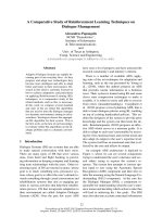
In order to optimize the running time of segmentation
and contour detection algorithms, we use a HS con-
structed on the image pixels, as presented in Figure 1.
Each hexagon represents an elementary item and the
entire HS represents a grid-graph, G =(V, E), where
each hexagon h in this structure has a corresponding
vertex v Î V. The set E of edges is constructed by con-
necting pairs of hexagons that are neighbors in a 6-con-
nected sense, because each hexagon has six neighbors.
The advantage of using hexagons instead of pixels as
elementary piece of information is that the amount of
memory space associated to the graph vertices is
reduced. Denoting by n
p
thenumberofpixelsofthe
initial image, the number of the resulted hexagons is
always less than n
p
= 4, and then the cardinal of both
sets V and E is significantly reduced.
We associate to each hexagon h from V two impor-
tant attributes representing its dominant color and t he
coordinates of its gravity center. For determining these
attributes, we use eight pixels contained in a hexagon h:
six pixels from the frontier and two interior pixels. We
select one of the two interior pixels to represent with
approximation the gravity center of the hexagon because

pixels from an image have integer values as coordinates.
We select always the left pixel from the two interior pix-
els of a hexagon h to represent the pseudo-center of the
gravity of h, denoted by g(h).
The dominant color of a hexagon is denoted by c(h)
and it represe nts the mean color v ector of the all eight
colors of its associated pixels. Each hexagon h in the
hexagonal grid is thus represented by a single point, g
(h),6 having the color c(h).
The segmentation system creates an HS on the pixels
of the input image and an undirected grid graph having
hexagons as vertices, and uses this graph in order to
produce a set of salient objects contained in the image.
In order to allow an unitary processing for the multi-
level system at this lev el we store, for e ach determined
component C:
- an unique index of the component;
Figure 1 HS constructed on the image pixels.
Stanescu et al. EURASIP Journal on Advances in Signal Processing 2011, 2011:128
/>Page 4 of 12
- the set of the hexagons contained in the region asso-
ciated to C;
- the set of hexagons located at the boundary of t he
component.
In addition for each component a mean color of the
region is extracted. Our HS is similar to quincunx sam-
pling scheme, but there are some important differences.
The quincux sample grid is a sublattice of a square lat-
tice that retains half of the image pixels [34]. The key
point of our HS, that also uses half of the image pixels,

is that the hexagonal grid is not a lattice because hexa-
gons are not regular. Although our hexagonal grid is
not a hexagonal lattice, we use some of the advantages
of the hexagonal grid such as uniform connectivity. In
our case, only one type of neighborhood is possible,
sixth neighborhood structure, unlike several types as N4
and N8 in the case of square lattice.
3.1 Algorithms for computing the color of a hexagon and
the list of hexagons with the same color
The algorithms return t he list of salient regions from
the input image. This list is obtained using the hexago-
nal network and the distance betwe en two colors in the
RGB color space. In order to obtain the color of a hexa-
gon a procedure called sameVertexColour is used. This
procedure has a constant execution time because all
calls are constant in time processing. The color informa-
tion will be used by the procedure expandColorArea to
find the list of hexagons that have the same color.
3.1.1 Determination of the hexagon color
The input of this procedure contains the current hexa-
gon h
i
, L
1
–the colors list of pixels corresponding to the
hexagona l network: L
1
={p
1
, ,p

6n
}. The output is repre-
sented by the object crtColorHexagon.
Procedure sameVertexColour (h
i
, L
1
)
initialize
crtColorHexagon;
determine the colors for the six ver-
tices of hexagon h
i
determine the colors for the two ver-
tices from interior of hexagon h
i
calculate the mean color value meanCo-
lor for the eight colors of vertices;
crtColorHexagon.colorHexagon <-
meanColor;
crtColorHexagon:sameColor <- true;
for k <- 1 to 6 do
if colorDistance(meanColor, color-
Vertex[k]) > threshold then
crtColorHexagon:sameColor <-
false;
break;
end
end
return crtColorHexagon;

Intheabovefunction,thethresholdvalueisanadap-
tive one, defined as the sum between the average of the
color distances associated to edges (between the adja-
cent hexagons) and the standard deviation of these color
distances.
3.1.2 Expand the current region
The function expandColourArea is a depth-first traver-
sing procedure, which starts with an specified hexagon
h
i
, pivot of a region item, and determines the list of all
adjacent hexagons representing the current region con-
taining h
i
such that the color dissimilarity between the
adjacent hexagons is below a determined threshold.
The input parameters of this function is the current
region item, index-CrtRegion, its first hexagon, h
i
,and
the list of all hexagons V from the hexagonal grid.
Procedure expandColourArea (h
i
, crtRegionI-
tem, V)
push(h
i
);
while not(empty(stack)) do
h <- pop();

for each hexagon h
j
neighbor to h do
if not(visit (V[h
j
])) then
if colorDistance(h, h
j
) < threshold
then
add h
j
to crtRegionItem
mark visit (V[h
j
])
push (h
j
)
end
end
end
end
The running time of the procedure expandColourArea
is O(n)wheren is the number of hexagons from a
region with the same color [35].
3.2 The algorithm used to obtain the regions
The procedures presented above are used by the listRe-
gions procedure to obtain the list of regions.
This procedure has an input which contains the vector

V representing the list of hexagons and the list L
1
.
The output is represented by a list of colors pixels and
a list of regions for each color.
Procedure listRegions (V, L
1
)
colourNb <- 0;
for i <- 1 to n do
initialize crtRegionItem;
if not(visit( h_ i)) then
crtColorHexagon <- sameVer texCo-
lour (L
1
, h
i
);
if crtColorHexagon.sameColor then
k <- findColor(crtColorHexagon.
color);
if k < 0 then
Stanescu et al. EURASIP Journal on Advances in Signal Processing 2011, 2011:128
/>Page 5 of 12
add new color ccolourNb to list C;
k <- colourNb++;
indexCrtRegion <- 0;
else
indexCrtColor <- k;
indexCrtRegion<-

findLastIndexRegion(index
CrtColor);
indexCrtRegion++;
end
hi.indexRegion <- indexCrtRegion;
hi.indexColor <- k;
add h
i
to crtRegionItem;
expandColourArea(h
i
, L
1
,V,
indexCrtRegion, indexCrtColor,
crtRegionItem);
add new region crtR egionItem to
list of element k from C
end
end
end
The running time of the procedure list Regions is O(n)
2
, where n is the number of the hexagons network [35].
Let G =(V, E) be the initial graph constructed on the
HS of an image. The color-based sequence of segmenta-
tions, S
i
=(S
0

, S
1
, , S
t
), will be generated by using a
color-based region model and a maximum spanning
tree construction method based on a modified form of
the Kruskal’s algorithm [36].
In the color-based region model, the evidence for a
boundary between two regions is based on the d iffer-
ence between the internal contrast of the regions and
the external contrast between them. Both notions of
internal contrast or internal variation of a component,
and external contrast or external variation between two
components are based on the dissimilarity bet ween two
colors [37]:
ExtVar(C

, C

)= max
(h
i
,h
j
)∈cb(c

,c

)

w(h
i
, h
j
)
(3)
IntVar(C)= max
(h
i
,h
j
)∈c
w(h
i
, h
j
)
(4)
where cb(C’, C“) represents the common boundary
between the components C’ and C“ and w is the color
dissimilarity between two adjacent hexagons:
w(h
i
, h
j
)=PED(c(h
i
), c(h
j
))

(5)
where c(h) represents the mean color vector associated
with the hexagon h.
The maximum internal contrast between two compo-
nents is defined as follows [37]:
IntVar(C

, C

)=max(IntVar(C

), IntVar(C

)) + r
(6)
where the threshold r is an adaptive value defined as
the sum between the average of the c olor distances
associated to edges and the standard deviation, r = μ +
s.
The comparison predicate between two neighboring
components C’ and C“ determines if there is an evi-
dence for a boundary between them [37].
dif f
col
(C

, C

)=


true, ExtVar(C

, C

) > IntVar(C

, C

)
false, ExtVar(C

, C

) ≤ IntVar(C

, C

)
(7)
The color-based segmentation algorithm represents an
adapted form of a Kruskal’s algorithm and it builds a
maximal spanning tree for each salient region of the
input image.
4 The color set back-projection algorithm
Color sets provide an alternative to color histograms for
representing color information. Their utilization is based
on the assumption that salient regions have not more
than few equally prominent colors [38].
The color set back-projection algorithm proposed in
[38] is a t echnique for the automated extraction o f

regions and representation of their color content.
The back-projection process requires several stages:
color set selection, back-projection onto the image,
thresholding, and labeling. Candidate color sets are
selected first with one color, then with two colors, etc.,
until the salient regions are extracted. For each image
quantization of the RGB color space at 64 colors is
performed.
The algorithm follows the reduction of insignificant
color information and makes evident the significant CS,
followed by the generation, in automatic way, of the
regions of a single color, of the two colors, etc.
For each detected region the color set, the area and
the localization are stored. The region localization is
given by the minimal bounding r ectangle. The region
area is represented by the number of color pixels, and
can be smaller than the minimum bounding rectangle.
The image processing algorithm computes both the
global histogram of the image, and the binary color set
[7,32]. The quantized colors are stored in a matrix. To
this matrix a 5 × 5 median filter is applied which has
the role of eliminating the isolated points. The process
of regions extraction is using the filtered matrix and it
is a depth-first traversal described in pseudo-code in the
following way:
Procedure FindRegions (Image I, colorset
C)
InitStack(S)
Visited = ∅
Stanescu et al. EURASIP Journal on Advances in Signal Processing 2011, 2011:128

/>Page 6 of 12
for *each node P in I do
if *color of P is in C then
PUSH(P)
Visited <- Visited ∪ P
while not Empty(S) do
CrtPoint <- POP()
Visited <- Visited ∪ CrtPoint
For *each unvisited neighbor S o f
CrtPoint do
if *color of S is in C then
Visited <- Visited ∪ S
PUSH(S)
end
end
end
* Output detected region
end
end
The total running time for a call of the procedure Fin-
dRegions (Image I, colorset C) is O(m
2
× n
2
) where m is
the width and n is the height of the image [7,32].
5 Local variation algorithm
This algorithm described in [20] is using a graph-based
approach for the image segmentation process. The pix-
els are considered the graph nodes so in this way it is

possible to define an undirected graph G =(V, E)where
the vertices v
i
from V representthesetofelementsto
be segmented. Each edge (v
i
, v
j
) belonging to E has asso-
ciated a corresponding weight w(v
i
, v
j
) calculated based
on color, which is a measure o f the dissimilarity
between neighboring elements v
i
and v
j
.
A minimum spanning tree is obtained using Kruskal’s
algorithm [36]. The connected components that are
obtained represent image regions. It is supposed that
the graph has m edges and n vertices. This algorithm is
described also in [39] where i t has four major steps that
are presented below:
Sort E=(e
1
, , e
m

) such that |e
t
|<
|e

t
|
∪ t
<t’
Let S
0
=({x
1
}, , {x
n
}) be each initial
cluster containing only one vertex.
For t = 1, , m
Let x
i
and x
j
be the vertices con-
nected by e
t
Let
C
t−1
xi
be the connected component

containing point x
i
on iteration t-1 and
l
i
= max
mst
C
t−1
xi
be the longest edge in
the minimum spanning tree of
C
t−1
xi
. Likewise
for l
j
.
Merge
C
t−1
xi
and
C
t−1
xj
if
|e
t

| < min{l
i
+
k
C
t−1
xi
, l
j
+
k
C
t−1
xj
}
where k is a
constant.
S = S
m
The existence of a boundary between two components
in segmentation is based on a predicate D.Thispredi-
cate is measuring the dissimilarity between elements
along the boundary of the two componen ts relative to a
measure of the dissimilarity among neighboring ele-
ments within each of the two compone nts. The internal
difference of a component C ⊆ V was defined as the lar-
gest weight in the minimum spanning tree of a compo-
nent MST(C, E):
Int(C)=max
e∈MST(CE)

w(e)
(8)
A threshold function is used to control the degree to
which the difference between components must be lar-
ger than minimum internal difference. The pa irwise
comparison predicate is defined as:
D(C
1
, C
2
)=

true, ifDif (C
1
, C
2
) > MInt(C
1
, C2)
false, otherwise
(9)
where the minimum internal difference Mint is
defined as:
MInt(C
1
, C
2
)=min(Int(C
1
)+τ (C

1
), Int(C
2
)+τ (C
2
))
(10)
The threshold function was defined based on the size
of the component: τ(C)=k/|C|. The k value is set taking
into account the size of the image. For images having
the size 128 × 128 k is set to 150 and for images with
size 320 × 240 k is set to 300. The algorithm for creat-
ing the minimum spanning tree can be implemented to
run in O(m log m)wherem is the number of edges in
the graph. The input of the algo rithm is represented by
agraphG =(V, E)withn vertices and m edges. The
obtained output i s a segmentation of V in the compo-
nents S =(C
1
, , C
r
). The algorithm has five major steps:
Sort E into π =(o
1
,,o
tπ
) by non-decreas-
ing edge weight
Start with a segm entation S
D

, where each
vertex v
i
is in own component
Repeat step 4 for $q = 1, . . . , m$
Construct S
q
using S
q
-1
and the internal
difference. If v
i
and v
j
areindisjointcom-
ponents of S
q
-1
and the weight of t he edge
between v
i
and v
j
is small compared to the
internal difference then merge the two com-
ponents otherwise do nothing.
Return S = S
tπ
Unlike the classica l methods this technique adaptively

adjusts the segmentation criterion based on the degree
of variability in neighboring regions of the image.
Stanescu et al. EURASIP Journal on Advances in Signal Processing 2011, 2011:128
/>Page 7 of 12
6 Segmentation error measures
A potential user of an algorithm’s output needs to know
what types of i ncorrect/invalid results to expect, as
some types of results might be acceptable while others
are not. T his called for the use o f metrics that are
necessary for potential consumers to make intelligent
decisions.
This section presents the characteristics of the error
metrics defined in [4]. The authors proposed two
metrics that can be used to evaluate the consistency of a
pair of segmentations, where segmentation is simply a
division of the pixels of an image into sets. Thus a seg-
mentation error measure takes two segmentations S1
and S2 as input and produces a real valued output in
the range [0 1] where zero signifies no error.
The process defines a measure of error at each pixel
that is tolerant to refinement as the basis of both mea-
sures. A given pixel pi is defined in relation to the seg-
ments in S1 and S2 that contain that pixel. As the
segments are sets of pixels and one segment is a prop er
subset of the other, then the pixel lies in an area of
refinement and the local error should be zero. If there is
no subset relationship, then the two regions overlap in
an inconsistent manner. In this case, the local error
should be non-zero. Let \ denote set difference, and |x|
the cardinality of set x. If R(S,pi) is the set of pixels cor-

responding to the region in segmentation S that con-
tains pixel pi, the local refinement error is defi ned as in
[4]:
E(S1, S2, pi)=
|R(S1, pi)/R(S2, pi)|
|R(S1, pi)|
(11)
Note that this local error measure is not symmetric. It
encodes a measure of refinement in one direction only:
E(S1, S2, pi) is zero precisely when S1 is a refinement of
S2 at pixel pi, but not vice versa. Given this local refine-
ment error in each direction at each pixel, there are two
natural ways to combine the values into an error mea-
sure for the entire image. GCE forces all local refine-
ments to be in the same direction. Let n be the number
of pixels:
GCE(S1, S2) =
1
n
min{

i
E(S1, S2, pi),

i
E(S2, S1, pi)}
(12)
LCE allows refinement in different directions in differ-
ent parts of the image.
LCE(S1,S2) =

1
n

i
min{E(S1, S2, pi), E(S2, S1, pi)}
(13)
As LCE ≤ GCE for any two segmentations, it is clear
that GCE is a tougher measure than LCE. Martin et al.
showed that, as expected, when pairs of human
segmentations of the same image are compared, both
the GCE and the LCE are low; conversely, when random
pairs of human segmentations are compared, the result-
ing GCE and LCE are high.
7 Experiments and results
This section presents the experimental results for the
evaluation of the three segmentation algorithms and
error measures values.
The experiments were made on a database with 500
medical images from digestive area captured by an
endoscope. The images were taken from patients having
diagnoses such as polyps, ulcer, esopha gites, coliti s, and
ulcerous tumors.
For each image, the following steps are performed by
theapplicationthatwehavecreatedtocalculatethe
GCE and LCE values:
Obtain the image regions using the color set back-
projection segmentation
Obtain the image regions using the LV
Obtain the image regions using the algorithm based
on the HS

Obtain the manually segmented regions
Store these regions in the database
Calculate GCE and LCE
Store these values in the database for later statistics
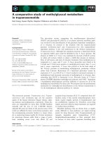
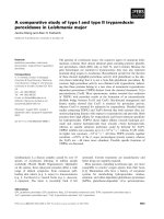
In Figure 2 the images for which we present some
experimental results are presented. Figures 3 and 4 pre-
sent the regions resulted from manual segmentation and
from the application of the three algorithmspresented
above for the images displayed in Figure 2.
In Table 1 the number of regions resulted from the
application of the segmentation can be seen.
In Table 2 the GCE values calculated for each algo-
rithm are presented.
In Table 3 the LCE values calculated for each algo-
rithm are presented.
If two different segmentations arise from different per-
ceptual organizations of the scene, then it is fair to
declare the segmentations inconsistent. If, however, seg-
mentation is simply a refinement of the other, then the
error should be small, or even zero. The error measures
presented in the above tables are calculated in r elation
with the manual segmentation which is considered true
segmentation. From Tables 2 and 3 it can be observed
that the values for GCE and LCE are lower in the case
of hexagonal segmentation. The error measures, for
almost all tested images, have smaller values in the case
of the original segmentation method which use a HS
defined on the set of pixels.
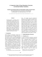
Figure 5 presents the repartition of the 500 images
from the database on GCE values. The focus point here

isthenumberofimagesonwhichtheGCEvalueis
under 0.5.
Stanescu et al. EURASIP Journal on Advances in Signal Processing 2011, 2011:128
/>Page 8 of 12
Figure 2 Images used in experiments.
Figure 3 The resulted regions for image no. 1.
Stanescu et al. EURASIP Journal on Advances in Signal Processing 2011, 2011:128
/>Page 9 of 12
In conclusion, for HS algorithm, a number of 391
images (78%) obtained GCE values under 0.5. Similarly,
for CS algorithm only 286 images (57%) obtained GCE
values under 0.5. The segmentation based on LV
method is close to our original algorithm: 382 images
(76%) had GCE values under 0.5.
Because the error measures for segmentation using a
HS defined on the set of pixels are lower than for color
set back-projection and local variation segment ation, we
can infer that t he segmentation method based on HS is
more efficient.
Experimental result s show that the original segmenta-
tionmethodbasedonaHSisagoodrefinementofthe
manual segmentation.
8 Conclusion
The aim of this article is to evaluate three algorithms
able to detect the regions in endoscopic images: a
Figure 4 The resulted regions for image no. 2.
Table 1 The number of regions detected for each
algorithm
Image number CS LV HS MS
19534

28723
Table 2 GCE values calculated for each algorithm
Image number GCE-CS GCE-LV GCE-HS
1 0.18 0.24 0.09
2 0.36 0.28 0.10
Table 3 LCE values calculated for each algorithm
Image number LCE-CS LCE-LV LCE-HS
1 0.11 0.15 0.07
2 0.18 0.17 0.12
Stanescu et al. EURASIP Journal on Advances in Signal Processing 2011, 2011:128
/>Page 10 of 12
clustering method (the color set back-projection algo-
rithm), as well as other two methods of segmentation
based on graphs: the LV and our original segme ntation
algorithm.
Our method is based on an HS defined on the set of
image pixels. The advantage of using a virtual hexagonal
network superposed over the initial im age pixels is that
it reduces the execution time and the memory space
used, without loosing the initial resolution of the image.
In comparison to other segmentation methods, our
algorithm is able to adapt and does not require neither
parameters for establishing the optimal values, nor sets
of training images to set parameters.
Furthermore, the article presents a method that
enables the assessment of the segmentation accuracy.
The role of this review is to find out which segmenta-
tion algorithm gives the best results for medical images
from digestive area captured by an endoscope.
First, the correctness of segments resulted after the

application of the three algorithms described above is
compared. Concerning the endoscopic database all the
algorithms have the ability to produce segmentations
that comply with the manual segmentation made by a
medical expert. Then for evaluating the accuracy of the
segmentation error measures are used. The proposed
error measures quantify the consistency between seg-
mentations of differing granularities. Because human
segmentation is considered true segmentation the error
measures are calculated in relation with manual seg-
mentation. The GCE and LCE demonstr ate that the
image segmentation based on an HS produces a better
segmentation than the back-projection method and the
LV.
The future research will focus on developing our seg-
mentation algorithm so as to include the texture feature
along with the color feature and reducing the algorithm
complexity at O(n log n), where n represents the num-
ber of image pixels.
Acknowledgements
The support of The National University Research Council under Grant CNC-
SIS IDEI 535 is gratefully acknowledged.
Competing interests
The authors declare that they have no competing interests.
Received: 15 May 2011 Accepted: 9 December 2011
Published: 9 December 2011
References
1. DL Pham, C Xu, JL Prince, Current methods in medical image
segmentation. Annu Rev Biomed Eng. 2, 315–337 (2000). doi:10.1146/
annurev.bioeng.2.1.315

2. L Stanescu, D Burdescu, M Brezovan, in Chapter Book: Multimedia Medical
Databases, Biomedical Data and Applications, Series: Studies in Computational
Intelligence, vol. 224, ed. by Sidhu AS, Dillon T, Bellgard M (Springer, 2009)
3. SK Warfield, KH Zou, WM Wells, Simultaneous truth and performance level
estimation (STAPLE): an algorithm for the validation of image segmentation.
Med Imag IEEE Trans. 23(7), 903–921 (2004). doi:10.1109/TMI.2004.828354
4. D Martin, C Fowlkes, D Tal, J Malik, A database of human segmented
natural images and its application to evaluating segmentation algorithms
and measuring ecological statistics, in Proceedings of the Eighth International
Conference On Computer Vision (ICCV-01). 2, 416–425 (2001)
5. DD Burdescu, L Stanescu, A new algorithm for content-based region query
in databases with medical images, in Conference of International Council on
Medical and Care Compunetics, Symposium On Virtual Hospitals, Symposium
on E-Health, Proceedings in Studies In Health Technology and Informatics. 114,
132–133 (2005). Medical and Care Compunetics 2
6. DD Burdescu, L Stanescu, A new algorithm for content-based region query
in multimedia database, in 16th International Conference on Database and
Expert Systems Applications, Proceedings in Lectures Notes in Computer
Science. 3588, 124–133 (2005)
7. DD Burdescu, L Stanescu, Color image segmentation applied to medical
domain. Intell Data Eng Autom Learn. 4881, 457–466 (2007). doi:10.1007/
978-3-540-77226-2_47
8. L Stanescu, DD Burdescu, Medical image segmentation–a comparison of
two algorithms, in International Workshop on Medical Measurements and
Applications (2010)
9. JR Smith, Integrated spatial and feature image systems: retrieval,
compression and analysis, PhD thesis, Graduate School of Arts and Sciences
Columbia University, (1997)
10. H Muller, N Michoux, D Bandon, A Geissbuhler, A review of content-based
image retrieval systems in medical applications–clinical benefits and future

directions. Int J Med Inf. 73(1), 1–23 (2004). doi:10.1016/j.
ijmedinf.2003.11.024
11. C Jiang, X Zhang, M Christoph, Hybrid framework for medical image
segmentation. Lecture Notes in Computer Science. 3691, 264–271 (2005).
doi:10.1007/11556121_33
Figure 5 Number of images relative to GCE values.
Stanescu et al. EURASIP Journal on Advances in Signal Processing 2011, 2011:128
/>Page 11 of 12
12. S Belongie, C Carson, H Greenspan, J Malik, Color and texture-based image
segmentation using the expectation-maximization algorithm and its
application to content-based image retrieval. in ICCV 675–682 (1998)
13. C Carson, S Belongie, H Greenspan, J Malik, Blobworld: image segmentation
using expectation-maximization and its application to image querying. IEEE
Trans Pattern Anal Mach Intell. 24(8), 1026–1038 (2002). doi:10.1109/
TPAMI.2002.1023800
14. L Ballerini, Medical image segmentation using Genetic snakes, Applications
and Science of Neural Networks, Fuzzy Systems, and Evolutionary Computation
II, (Denver Co, 1999)
15. S Ghebreab, AWM Smeulders, Medical images segmentation by strings, in
Proceedings of the VISIM Workshop: Information Retrieval and Exploration in
Large Collections of Medical Images (2001)
16. S Ghebreab, AWM Smeulders, An approximately complete string
representation of local object boundary features for concept-based image
retrieval, in IEEE International Symposium on Biomedical Imaging (2004)
17. S Gordon, G Zimmerman, H Greenspan, Image segmentation of uterine
cervix images for indexing in PACS, in Proceedings of the 17th IEEE
Symposium on Computer-Based Medical Systems, CBMS (2004)
18. H Lamecker, T Lange, M Seeba, S Eulenstein, M Westerhoff, HC Hege,
Automatic segmentation of the liver for preoperative planning of
resections, in Proceedings of Medicine Meets Virtual Reality, Studies in Health

Technologies and Informatics. 94, 171–174 (2003)
19. H Muller, S Marquis, G Cohen, PA Poletti, CL Lovis, A Geissbuhler, Automatic
abnormal region detection in lung CT images for visual retrieval. Swiss Med
Inf. 57,2–6 (2005)
20. PF Felzenszwalb, WD Huttenlocher, Efficient graph-based image
segmentation. Int J Comput Vis. 59(2), 167–181 (2004)
21. L Guigues, LM Herve, LP Cocquerez, The hierarchy of the cocoons of a
graph and its application to image segmentation. Pattern Recogn Lett.
24(8), 1059–1066 (2003). doi:10.1016/S0167-8655(02)00252-0
22. J Shi, J Malik, Normalized cuts and image segmentation. in Proceedings of
the IEEE Conference on Computer Vision and Pattern Recognition 731–737
(1997)
23. Z Wu, R Leahy, An optimal graph theoretic approach to data clustering:
theory and its application to image segmentation. IEEE Trans Pattern Anal
Mach Intell. 15(11), 1101–1113 (1993). doi:10.1109/34.244673
24. C Zahn, Graph-theoretical methods for detecting and describing gestal
clusters. IEEE Trans Comput. 20(1), 68–86 (1971)
25. R Urquhar, Graph theoretical clustering based on limited neighborhood
sets. Pattern Recogn. 15(3), 173–187 (1982). doi:10.1016/0031-3203(82)
90069-3
26. Y Gdalyahu, D Weinshall, M Werman, Self-organization in vision: stochastic
clustering for image segmentation, perceptual grouping, and image
database organization. IEEE Trans Pattern Anal Mach Intell. 23(10),
1053–1074 (2001). doi:10.1109/34.954598
27. I Jermyn, H Ishikawa, Globally optimal regions and boundaries as minimum
ratio weight cycles. IEEE Trans Pattern Anal Mach Intell. 23(8), 1075–1088
(2001)
28. M Cooper, The tractibility of segmentation and scene analysis. Int J Comput
Vis. 30(1), 27–42 (1998). doi:10.1023/A:1008013412628
29. T Pavlidis, Structural Pattern Recognition (Springer, 1977)

30. D Comaniciu, P Meer, Robust analysis of feature spaces: color image
segmentation. in Proceedings of the IEEE Conference on Computer Vision and
Pattern Recognition 750–755 (2003)
31. A Jain, R Dubes, Algorithms for Clustering Data (Prentice Hall, 1988)
32. L Stanescu, Visual Information. Procecessing, Retrieval and Applications
(Sitech, Craiova, 2008)
33. A Gijsenij, T Gevers, M Lucassen, A perceptual comparison of distance
measures for color constancy algorithms, in Proceedings of the European
Conference on Computer Vision. 5302, 208–2011 (2008)
34. X Zhang, X Wu, Image coding on quincunx lattice with adaptive lifting and
interpolation. in Data Compression Conference 193–202 (2007)
35. DD Burdescu, M Brezovan, E Ganea, L Stanescu, A new method for
segmentation of images represented in a HSV color space. in ACIVS
606–617 (2009)
36. MT Goodrich, R Tamassia, Data Structures and Algorithms in Java, 4th edn.
(John Wiley and Sons, Inc, 2006)
37. M Brezovan, DD Burdescu, E Ganea, L Stanescu, Boundary-based
performance evaluation of a salient visual object detection algorithm, in
Proceedings of the WorldComp IPCV (2010)
38. JR Smith, SF Chang, Tools and techniques for color image retrieval, Proc.
SPIE Storage retrieval for still image and video databases, IV. 2670, 426–437
(1996)
39. C Pantofaru, M Hebert, A comparison of image segmentation algorithms,
Technical Report CMU-RI-TR-05-40, Robotics Institute, Carnegie Mellon
University, Pittsburgh, PA, (2005)
doi:10.1186/1687-6180-2011-128
Cite this article as: Stanescu et al.: A comparative study of some
methods for color medical images segmentation. EURASIP Journal on
Advances in Signal Processing 2011 2011:128.
Submit your manuscript to a

journal and benefi t from:
7 Convenient online submission
7 Rigorous peer review
7 Immediate publication on acceptance
7 Open access: articles freely available online
7 High visibility within the fi eld
7 Retaining the copyright to your article
Submit your next manuscript at 7 springeropen.com
Stanescu et al. EURASIP Journal on Advances in Signal Processing 2011, 2011:128
/>Page 12 of 12