Báo cáo hóa học: " Hard versus fuzzy c-means clustering for color quantization" ppt
Bạn đang xem bản rút gọn của tài liệu. Xem và tải ngay bản đầy đủ của tài liệu tại đây (637.29 KB, 12 trang )
RESEARCH Open Access
Hard versus fuzzy c-means clustering for color
quantization
Quan Wen
1
and M Emre Celebi
2*
Abstract
Color quantization is an important operation with many applications in graphics and image processing. Most
quantization methods are essentially based on data clustering algorithms. Recent studies have demonstrated the
effectiveness of hard c-means (k-means) clustering algorithm in this domain. Other studies reported similar findings
pertaining to the fuzzy c-means algorithm. Interestingly, none of these studies directl y compared the two types of
c-means algorithms. In this study, we imp lement fast and exact variants of the hard and fuzzy c-means algorithms
with several initialization schemes and then compare the resulting quantizers on a diverse set of images. The
results demonstrate that fuzzy c-means is significantly slower than hard c-means, and that with respect to output
quality, the former algorithm is neither objectively nor subjectively superior to the latter.
1 Introduction
True-color images typically contain thousands of colors,
which makes their display, storage, transmission, and
processing problematic. For this reason, color quantiza-
tion (reduction) is commonly used as a preprocessing
step for various graphics and image processing tasks. In
the past, col or quantization was a necessity due to t he
limitations of the display hardware, which could not
handle over 16 million possible colors in 24-bit images.
Although 24-bit display hardware has be come more
common, color quantization still maintains its practical
value [1]. M odern applications of color quantization i n
graphics and image processing include: (i) compression
[2], (ii) segmentation [3], (iii) text localization/detection
[4], (iv) colo r-text ure analysis [5], (v) waterm arking [6],
(vi) non-photorealistic rendering [7], (vii) and content-
based retrieval [8].
The process of color quantization is mainly comprised
of two phases: palette design (the selection of a small
set of colors that represents the original image colors)
and pixel mapping (the assignment of each input pixel
to one of the palette colors). The primary objective is to
reduce the number of unique colors, N’,inanimageto
C, C ≪ N’, with minimal distortion. In most applica-
tions, 24-bit pixels in the original image are reduced to
8 bits or fewer. Since natural images often contain a
large number of colors, faithful representation of these
images with a limited size palette is a difficult problem.
Color quantization methods can be broadly classified
into two categories [9]: image-independent methods that
determine a universal (fixed) palette without regard to
any specific image [10] and image-dependent methods
that determine a custom (adaptive) palette based on the
color distribution of the images. Despite being very fast,
image-independent methods usually give poor results
since they do not take into account the image contents.
Therefore, most of the studi es in the liter atur e cons ider
only image-dependent methods, which strive to achieve
a better balance between computational efficiency and
visual quality of the quantization output.
Numerous image-dependent color quantization meth-
ods have been developed i n the past three decades.
These can be categorized into two families: preclustering
methods and postclustering methods [1]. Preclustering
methods are mostly based on the statistical analysis of
the color distribution of the images. Divisive precluster-
ing methods start with a single cluster that contains all
N’ image colors. This initial cluster is recursively subdi-
vided until C clusters are obtaine d. Well-known divisive
methods include median-cut [11], octree [12], variance-
based method [13], binary splitting method [14], and
greedy orthogonal bipartitioning method [15]. On the
other hand, agglomerative preclusterin g methods
[16-18] start with N’ singleton clusters each of which
* Correspondence:
2
Department of Computer Science, Louisiana State University, Shreveport,
LA, USA
Full list of author information is available at the end of the article
Wen and Celebi EURASIP Journal on Advances in Signal Processing 2011, 2011:118
/>© 2011 Wen and Celebi; licensee Springer. This is an Open Access article distributed under the terms of the Cre ative Commons
Attribution License ( whi ch permits unrestricted use, distribution, and reproduction in
any medium, provid ed the original work is properly cited.
contains one image color. These clusters are repeatedly
merged until C clusters remain. In contrast to preclus-
tering methods that compu te the palette only once,
postclustering methods first determine an initial palette
and then improve it iteratively. Essentially, any data
clustering method can be used for this p urpose. Since
these methods involve iterative or stochastic optimiza-
tion, they can obtain higher quality results when com-
pared to preclustering methods at the expense of
increased computational time. Clustering algorithms
adapted to color quantization include hard c-means
[19-22], competitive learning [23-27], fuzzy c-means
[28-32], and self-organizing maps [33-35].
In this paper, we compare the performance of hard
and fuzzy c-means algorithms within the context of
color quantization. We implement several ef ficient var-
iants of both algorithms, each one with a different initia-
lization scheme, and then compare the resulting
quantizers on a diverse set of images. The rest of the
paper is organized as follows. Section 2 reviews the
notions of hard and fuzzy partitions and gives an over-
view of the hard and fuzzy c-means algorithms. Section
3 describes the experimental setup and compares the
hard and fuzzy c-means variants on the test images.
Finally, Sect. 4 gives the conclusions.
2 Color quantization using c-means clustering
algorithms
2.1 Hard versus fuzzy partitions
Given a data set X ={x
1
, x
2
, ,x
N
} Î ℝ
D
,areal
matrix U =[u
ik
]
C×N
represents a hard C-partition of X
if and only if its elements satisfy three conditions [36]:
u
ik
∈{0, 1} 1 ≤ i ≤ C,1≤ k ≤ N
C
i=1
u
ik
=1 1≤ k ≤ N
0 <
N
k=1
u
ik
< N 1 ≤ i ≤ C.
(1)
Row i of U,sayU
i
=(u
i1
, u
i2
, ,u
iN
), exhibits the
characteristic function of the ith partition (cluster) of X:
u
ik
is 1 if x
k
is in the ith partition and 0 otherwise;
C
i=1
u
ik
=1 ∀k
means that each x
k
is in exactly one
of the C partitions;
0 <
N
k=1
u
ik
< N ∀i
means that
no partition is empty and no partition is all of X,i.e.2
≤ c ≤ N. For obvious reasons, U is often called a parti-
tion (membership) matrix.
The concept of hard C-partition can be generalized by
relaxing the first condition in Equation 1 as u
ik
Î 0[1]
in which case the partition matrix U is said to represent
a fuzzy C-partition of X [37]. In a fuzzy partition matrix
U, the total membership of each x
k
is still 1, but since 0
≤ u
ik
≤ 1 ∀i, k, it is possible for each x
k
to have an arbi-
trary distribution of membership among the C fuzzy
partitions {U
i
}.
2.2 Hard c-means (HCM) clustering algorithm
HCMisinarguablyoneofthemostwidelyusedmeth-
ods for data clustering [38]. It attempts to generate opti-
mal hard C-partitions of X by minimizing the following
objective functional:
J(U, V)=
N
k=1
C
i=1
u
ik
(d
ik
)
2
(2)
where U is a hard partition matrix as defined in §2.1, V
={v
1
, v
2
, ,v
C
} Î ℝ
D
is a set of C cluster representa-
tives (centers), e.g. v
i
is the center of hard cluster U
i
∀i,
and d
ik
denotes the Euclidean
(L
2
)
distance between
input vector x
k
and cluster center v
i
, i.e. d
ik
=||x
k
- v
i
||
2
.
Since u
ik
=1⇔ x
k
Î U
i
, and is zero otherwise, Equa-
tion 2 can also be written as:
J(U, V)=
C
i=1
x
k
∈U
i
(d
ik
)
2
.
Thi s problem is known to be NP-hard even for C =2
[39] or D = 2 [40], but a heuristic method developed by
Lloyd [41] offers a simple solution. Lloyd’s algorithm
starts with C arbitrary centers, typically chosen uni-
formly at random from the data points. Each point is
then assigned to the nearest center, and each center is
recalculated as the mean of all points assigned to it.
These two steps are repeated until a predefined termina-
tion criterion is met.
The complexity of HCM is
O(NC)
per iteration for a
fixed D value. In color quantization applications, D
often equals three since the clustering procedure is
usually performed in a three-dimensional color space
such as RGB or CIEL * a * b * [42].
From a cl ustering perspective, HCM has the fo llowing
advantages:
◊ It is conceptually simple, versatile, and easy to
implement.
◊ It has a time complexity that is linear in N and C.
◊ It is guaranteed to terminate [43] with a quadratic
convergence rate [44].
Due to its gradient descent nature, HCM often con-
verges to a local minimum of its objective functional
[43] and its output is highly sensitive to the selection of
the initial cluster centers. Adverse effects of improper
initialization include empty clusters, slower convergence,
and a higher chance of getting stuck in bad local
minima. From a color quantization perspective, HCM
Wen and Celebi EURASIP Journal on Advances in Signal Processing 2011, 2011:118
/>Page 2 of 12
has two additional drawbacks. First, despite its linear
time complexity, the iter ative nature of the algorithm
renders the palette generation phase computationally
expensive. Second, the pixel mapping phase is ineffi-
cient, since for each input pixel a full search of the pal-
ette is required to determine the nearest color. In
contrast, preclustering methods often manipulate and
store the palette in a special data structure (binary trees
are commonly used), which allows for fast nearest
neighbor search during the mapping phase. Note that
these drawbacks are shared by the majority of postclus-
tering methods, including the fuzzy c-means algorithm.
We have recently proposed a fast and exact HCM var-
iant called Weighted Sort-Means (WSM) that utilizes
data reduction and accelerated nearest neighbor search
[21,22]. When initialized with a suitable preclustering
method, WSM has b een shown to outperform a large
number of classic and state-of-the-art quantization
methods including median-cut [11], octree [12], var-
iance-based method [ 13], binary splitting method [14],
greedy orthogonal bipartitioning method [15], neu-
quant [33], split and merge method [18], adaptive distri-
buting units method [23,26], finite-state HCM me thod
[19], and stable-flags HCM method [20].
In this study, WSM is used in place of HCM since
both algorithms give numerically identical results. How-
ever, in t he remainder of this paper, WSM will be
referred to as HCM for reasons of uniformity.
2.3 Fuzzy c-means (FCM) clustering algorithm
FCM is a generalization of HCM in which points can
belong to more than one cluster [36]. It attempts to
generate optimal fuzzy C-partitions of X by minimizing
the following objective functional:
J
m
(U, V)=
N
k=1
C
i=1
(u
ik
)
m
(d
ik
)
2
(3)
where the parameter 1 ≤ m < ∞ controls the degree of
membership sharing between fuzzy clusters in X.
As in the case of HCM, FCM is based on an alter nat-
ing minimization procedure [45]. At each iteration, the
fuzzy partition matrix U is updated by
u
ik
=
⎡
⎣
C
j=1
d
ik
d
jk
2/(m−1)
⎤
⎦
−1
.
(4)
which is followed by the update of the proto type
matrix V by
v
i
=
N
k=1
(u
ik
)
m
x
k
/
N
k=1
(u
ik
)
m
.
(5)
As
m
+
→
1
, FCM converges t o an HCM solution.
Conversely, as m ® ∞ it can be shown that u
ik
® 1/C
∀i, k,so
v
i
→
¯
X
, the centroid of X. In general, the larger
m is, the fuzzier are the membership assignments; and
conversely, as
m
+
→
1
, FCM solutions b ecome hard. In
color quantization applications, in order to map each
input color to the nearest (most similar) palette color,
the membership values should be defuzzified upon con-
vergence as follows:
ˆ
u
ik
=
⎧
⎨
⎩
1 u
ik
=max
1≤j≤C
u
jk
0otherwise
.
A näive implementation of FCM has a complexity of
O(NC
2
)
per iteration, which is quadratic in the number
of clusters. In this study, a linear complexity formula-
tion, i.e.
O(NC)
, described in [46] is used. In order to
take advantage of the peculiarities of color image data
(pr esence of duplicate samples, limited range, and spar-
sity), the same data reduction strategy used in WSM is
incorporated into FCM.
3 Experimental results and discussion
3.1 Image set and performance criteria
Six publicly available, true-color images were used in the
experim ents. Five of these were natural images from the
Kodak Lossless True Color Image Suite [47]: Hats (768 ×
512; 34,871 unique colors), Motocross (768 × 512;
63,558 unique colors), Flowers and Sill (768 × 512;
37,552 unique colors), Cover Girl (768 × 512; 44,576
unique colors), and Parrots (768 × 512; 72,079 unique
colors). The sixth image w as synthetic, Poolballs (510 ×
383; 13,604 unique colors) [48]. The images are shown
in Figure 1.
The effectiveness of a quantization method was quan-
tified by the commonly used mean absolute error
(MAE) and mean squared error (MSE) measures:
MAE
I,
ˆ
I
=
1
HW
H
h=1
W
w=1
I(h, w) −
ˆ
I(h, w)
1
MSE
I,
ˆ
I
=
1
HW
H
h=1
W
w=1
I(h, w) −
ˆ
I(h, w)
2
2
(6)
where I and
ˆ
I
denote, respectively, the H × W original
and quantized images in the RGB color space. MAE and
MSE represent the average color distortion with respect
to the
L
1
(City-block) and
L
2
2
(squared Euclidean)
norms, respectively. Note that most of the other popular
evaluation measures in the color quantization literature
such as peak signal-to-noise ratio (PSNR), normalized
Wen and Celebi EURASIP Journal on Advances in Signal Processing 2011, 2011:118
/>Page 3 of 12
MSE, root MSE, and average color distortion [24,34] are
variants of MAE or MSE.
The efficiency of a quantization method was measured
by CPU time in milliseconds, which includes the time
required for both the palette generation and the pixel
mapping phases. The fast pixel mapping algorithm
described in [49] was used in the experiments. All of
the programs were implemented in the C language,
compiled with the gcc v4.4.3 compiler, and executed on
an Intel Xeon E5520 2.26 GHz machine. The time fig-
ures were averaged over 20 runs.
3.2 Comparison of HCM and FCM
The following well-known preclustering methods were
used in the experiments:
• Median-cut (MC) [11]: This method starts by
building a 32 × 32 × 32 color histogram that con-
tains the original pixel values reduced to 5 bits per
channel by uniform quantization (bit-cutting). This
histogram volume is then recursively split into smal-
ler boxes until C boxes are obtained. At each step,
the box that contains the largest number of pixels is
split along the longest axis at the median point, so
that the resulting sub-boxes each contain approxi-
mately the same number of pixels. The centroids of
the final C boxes are taken as the color palette.
• Octree (OCT) [12]: This two-phase method first
builds an octree (a tree data structure in wh ich each
internal node has u p to eight children) that
represents the color distribution of the input image
and then, starting from the bottom of the tree,
prunes the tree by merging its nodes until C colors
are obtained. In the experiments, the tree depth was
limited to 6.
• Variance-based method (WAN) [13]: This
method is similar to MC with the exception that at
each step the box with the largest weighted variance
(squared error) is split along the major (principal)
axis at the point that minimizes the marginal
squared error.
• Greedy orthogonal bipartitioning method (WU)
[15]:ThismethodissimilartoWANwiththe
exception that at each step the box with the largest
weighted variance is split along the axis that mini-
mizes the sum of the variances on both sides.
Four variants of HCM/FCM, each one initialized with
a different preclustering method, were tested. Each var-
iant was executed until it converged. Convergence was
determined by the following commonly used criterion
[50]: (J
(i-1)
- J
(i)
)/J
(i)
≤ ε,whereJ
(i)
denotes the value o f
the objective functional (Eqs. (2) and (3) for HCM and
FCM, respectively) at the end of the ith iteration. The
convergence threshold was set to ε = 0.001.
The weighting exponent (m) value recommended for
color quantization applications ranges between 1.3 [30]
and 2.0 [31]. In the experiments, four different m values
were tested for each of the FCM variants: 1.25, 1.50,
1.75, and 2.00.
(f) Poolballs
(
e
)
Parrots
(a) Hats
(b) Motocross
(c) Flowers and Sill
(d) Cover Girl
Figure 1 Test images. a Hats, b Motocross, c Flowers and Sill, d Cover Girl, e Parrots, f Poolballs.
Wen and Celebi EURASIP Journal on Advances in Signal Processing 2011, 2011:118
/>Page 4 of 12
Table 1 MAE comparison of the quantization methods
Hats Motocross
HCM FCM HCM FCM
C Init 1.25 1.50 1.75 2.00 Init 1.25 1.50 1.75 2.00
32 MC 30 16 16 16 16 15 26 19 19 19 18 18
OCT 19 15 15 15 15 15 21 17 18 18 18 18
WAN 26 15 15 15 15 15 24 18 18 18 18 18
WU 18 15 15 15 15 15 21 18 18 17 17 18
64 MC 18 12 12 11 11 11 20 15 15 14 14 14
OCT 13 10 10 10 10 10 15 13 13 13 13 13
WAN 18 11 11 10 10 11 19 14 14 13 13 14
WU 12 10 10 10 10 10 15 13 13 13 13 13
128 MC 13 9 8 8 8 8 16 12 11 11 11 11
OCT 9 7 7 7 7 7 12 10 10 10 10 10
WAN 11 8 7 7 7 7 15 10 10 10 10 11
WU 9 7 7 7 7 7 12 10 10 10 10 10
256 MC 10 7 6 6 6 6 13 9 9 9 8 9
OCT655555988888
WAN955555128 8888
WU655555988888
Flowers and Sill Cover Girl
HCM FCM HCM FCM
C Init 1.25 1.50 1.75 2.00 Init 1.25 1.50 1.75 2.00
32 MC 20 14 14 14 13 13 22 16 15 14 14 14
OCT 15 12 12 12 12 12 17 14 14 14 13 13
WAN 17 12 12 12 12 12 18 14 14 14 14 14
WU 14 12 12 12 12 12 16 14 14 14 14 14
64 MC 14 11 10 10 10 10 16 11 11 11 11 10
OCT 11 9 9 9 9 9 12 10 10 10 10 10
WAN 12 9 9 9 9 9 15 11 11 10 10 11
WU 10 9 9 9 9 9 12 10 10 10 10 10
128 MC 12 8 8 8 7 7 13 9 8 8 8 8
OCT877777987778
WAN977777128 8888
WU877777988888
256 MC 9 6 6 6 6 6 11 7 7 6 6 6
OCT655555766666
WAN855555106 6666
WU655555766666
Parrots Poolballs
HCM FCM HCM FCM
C Init 1.25 1.50 1.75 2.00 Init 1.25 1.50 1.75 2.00
32 MC 28 21 21 20 21 21 12 9 9 9 7 7
OCT 24 20 20 20 20 20 8 6 6 6 6 6
WAN 25 21 20 20 20 20 11 6 6 6 6 6
WU 23 20 20 20 20 20 7 7 6 6 6 6
64 MC 22 15 15 15 15 15 9 6 6 6 5 5
OCT 18 15 15 15 15 15 5 4 4 3 3 4
WAN 19 15 15 15 15 15 9 4 4 4 4 4
WU 17 15 15 15 15 15 5 4 4 4 4 4
128 MC 16 12 12 12 12 12 7 5 5 5 4 3
Wen and Celebi EURASIP Journal on Advances in Signal Processing 2011, 2011:118
/>Page 5 of 12
Table 1 MAE comparison of the quantization methods (Continued)
OCT 14 11 11 11 11 11 3 2 2 2 2 2
WAN 15 11 11 11 11 12 9 3 3 3 3 3
WU 13 11 11 11 11 11 4 3 3 3 2 2
256 MC 13 9 9 9 9 9 7 4 3 3 3 2
OCT 10 9 8 8 9 9 2 2 2 2 2 2
WAN 12 9 9 9 9 9 8 2 2 2 2 2
WU 10 9 8 8 9 9 4 2 2 2 2 2
Table 2 MSE comparison of the quantization methods
Hats Motocross
HCM FCM HCM FCM
C Init 1.25 1.50 1.75 2.00 Init 1.25 1.50 1.75 2.00
32 MC 618 159 169 163 175 185 427 217 209 229 236 253
OCT 293 185 184 187 214 242 301 197 203 249 277 280
WAN 624 162 160 165 172 201 446 194 193 220 235 291
WU 213 157 157 156 163 172 268 191 191 194 198 208
64 MC 192 91 87 86 87 99 232 125 123 119 125 134
OCT 132 79 79 78 87 94 159 111 112 122 129 142
WAN 311 89 83 84 100 110 292 112 111 117 122 141
WU 103 72 75 75 79 85 147 109 109 111 121 126
128 MC 111 47 45 45 50 52 154 76 74 72 75 86
OCT 65 43 43 43 48 52 96 65 65 69 76 91
WAN 106 44 42 44 48 51 169 66 66 68 72 85
WU 52 38 40 40 42 46 87 63 63 65 70 84
256 MC 63 29 27 26 28 31 100 49 45 45 48 57
OCT 34 22 24 25 28 33 54 39 39 42 48 55
WAN 53 21 23 24 26 30 92 39 39 40 44 53
WU 30 21 23 23 25 28 51 38 38 39 43 50
Flowers and Sill Cover Girl
HCM FCM HCM FCM
C Init 1.25 1.50 1.75 2.00 Init 1.25 1.50 1.75 2.00
32 MC 257 117 117 114 112 120 269 142 132 127 130 135
OCT 155 102 102 102 109 120 182 127 127 128 131 137
WAN 198 102 100 101 107 114 230 126 127 129 133 137
WU 134 101 100 101 103 108 162 126 125 126 129 133
64 MC 113 66 64 64 65 70 145 79 78 76 80 85
OCT 88 58 57 58 66 75 105 72 72 75 78 87
WAN 98 56 55 56 59 64 157 75 75 77 83 88
WU 71 53 56 57 59 61 93 71 72 73 76 82
128 MC 84 42 39 38 39 43 104 52 45 44 47 56
OCT 47 33 33 34 37 42 62 42 42 44 47 52
WAN 57 29 32 33 35 39 102 44 43 45 50 57
WU 40 30 32 32 34 38 55 41 40 41 44 49
256 MC 48 23 24 23 24 27 68 32 29 28 29 34
OCT 26 19 21 21 24 27 36 25 25 25 29 33
WAN 37 18 20 20 22 25 63 26 25 26 28 32
WU 26 18 20 20 22 24 33 24 24 24 26 31
Parrots Poolballs
HCM FCM HCM FCM
C Init 1.25 1.50 1.75 2.00 Init 1.25 1.50 1.75 2.00
Wen and Celebi EURASIP Journal on Advances in Signal Processing 2011, 2011:118
/>Page 6 of 12
Table 2 MSE comparison of the quantization methods (Continued)
32 MC 418 240 240 241 274 285 136 74 72 71 66 61
OCT 342 247 246 246 255 265 130 74 67 75 85 88
WAN 376 246 239 246 254 263 112 49 49 50 52 54
WU 299 234 234 237 244 256 68 50 50 50 50 54
64 MC 274 137 137 138 140 157 64 39 39 39 28 30
OCT 191 133 132 135 140 155 48 29 27 28 29 34
WAN 233 131 131 132 141 164 59 22 22 22 22 24
WU 167 130 130 131 135 155 31 22 21 21 22 23
128 MC 147 82 80 82 86 95 38 22 21 19 15 15
OCT 111 79 78 79 85 97 20 12 12 12 13 16
WAN 153 78 77 80 88 97 45 12 11 11 11 12
WU 95 77 77 78 83 91 17 11 10 10 11 11
256 MC 96 50 49 49 53 62 27 13 10 9 8 8
OCT 64 48 47 50 54 61 9 6 5 6 6 7
WAN 92 44 47 49 55 61 38 6 6 5 6 6
WU 58 46 46 48 52 59 11 6 5 5 6 6
Table 3 CPU time comparison of the quantization methods
Hats Motocross
HCM FCM HCM FCM
C 1.25 1.50 1.75 2.00 1.25 1.50 1.75 2.00
32 MC 48 2,664 3,238 3,192 934 84 11,797 7,749 9,244 1,895
OCT 80 1,883 2,032 1,656 691 110 4,139 5,034 4,054 912
WAN 45 3,406 2,709 2,980 762 60 4,261 2,971 4,013 715
WU 50 1,976 2,227 1,854 425 60 4,547 4,751 4,016 974
64 MC 59 10,536 11,059 5,494 1,211 101 29,081 24,021 24,858 5,640
OCT 97 5,045 7,353 5,533 1,379 130 10,154 8,752 9,366 1,857
WAN 62 9,350 9,729 10,303 1,501 94 12,531 8,842 10,308 3,160
WU 54 4,228 4,756 4,822 1,332 71 6,361 6,903 8,441 2,020
128 MC 108 20,269 19,945 15,815 2,879 156 49,930 54,102 57,146 14,704
OCT 141 12,700 11,745 8,799 2,444 180 22,410 20,504 18,866 5,297
WAN 89 22,871 13,143 11,544 2,071 125 17,472 19,467 23,061 5,683
WU 76 12,719 11,191 11,114 2,300 113 15,604 14,833 13,684 5,049
256 MC 267 42,670 51,559 35,602 6,126 607 144,758 116,915 131,130 28,752
OCT 306 20,287 19,512 17,806 5,039 328 39,101 42,906 37,946 7,988
WAN 202 26,505 20,574 18,794 5,649 380 50,621 45,127 38,105 9,152
WU 191 19,058 20,692 18,763 5,434 284 39,098 43,176 32,835 8,767
Flowers and Sill Cover Girl
HCM FCM HCM FCM
C 1.25 1.50 1.75 2.00 1.25 1.50 1.75 2.00
32 MC 56 5,591 5,633 5,243 1,385 55 6,067 6,772 7,402 1,545
OCT 81 2,618 4,151 3,447 645 82 1,992 2,615 2,026 584
WAN 42 2,240 2,525 2,625 709 45 1,934 1,988 1,975 613
WU 42 2,111 1,585 1,590 547 41 1,927 1,692 2,264 511
64 MC 62 10,508 9,098 8,938 1,970 77 14,165 24,945 18,248 4,979
OCT 99 9,091 6,579 7,396 1,369 100 6,431 6,775 4,570 1,803
WAN 58 5,413 4,060 4,491 1,067 59 6,540 9,785 7,905 2,574
WU 53 3,887 3,992 3,434 1,005 62 5,745 4,913 4,242 1,409
128 MC 124 35,372 31,854 28,658 4,198 120 47,186 45,248 34,731 9,428
Wen and Celebi EURASIP Journal on Advances in Signal Processing 2011, 2011:118
/>Page 7 of 12
Tables 1 and 2 compare the effectiveness of the HCM
and FCM variants on the test images. Similarly, Table 3
gives the efficiency comparison. For a given number of
colors C (C Î {32, 64, 128, 256}), preclustering method
P(P Î {MC, OCT, WAN, WU}), and input image I,the
column labeled as ‘Init’ contains the MAE/MSE between
I and
ˆ
I
(the output image obtained by reducing the
number of colors in I to C using P), whereas the one
labeled as ‘HCM’ contains the MAE/MSE value obtained
by HCM when initialized by P. The remaining four col-
umns contain the MAE/MSE values obtained by the
FCM variants. Note that HCM is equivalent to FCM
with m = 1.00. The following observations are in order
(note that each of these comparisons is made within the
context of a particular C, P, and I combination):
⊳ The most effective initialization method is WU,
whereas the least effective one is MC.
⊳ Both HCM and FCM reduces the quantization dis-
tortion regardless of the initialization method used.
However, the percentage of MAE/MSE reduction is
more significant for some initialization methods
than others. In general, HCM/FCM is more likely to
obtain a significant improvement in MAE/MSE
when initialized by an ineffective preclustering algo-
rithmsuchasMCorWAN.Thisisnotsurprising
given that such ineffective methods generate outputs
that are likely to be far from a local minimum, and
hence HCM/FCM can significantly improve upon
their results.
⊳ With respect to MAE, the HCM variant and the
four FCM variants have virtually identical
performance.
⊳ With respect to MSE, the performances of the
HCM variant and the FCM variant with m =1.25are
indistinguishable. Furthermore, the effectiveness of
the FCM variants degrades with increasing m value.
⊳ On average, HCM is 92 times faster than FCM.
This is because HCM uses hard memberships, which
makes possible various computational optimizations
tha t do not affec t accuracy of the algorithm [51-55].
On the o ther hand, due to the intensive fuzzy mem-
bership calculations involved, accelerating FCM is
significantly more difficult, which is why the major-
ity of existing acceleration methods involve approxi-
mations [56-60]. Note t hat the fast HCM/FCM
implementations used in this study give exactly the
same results as the conventional HCM/FCM.
Table 3 CPU time comparison of the quantization methods (Continued)
OCT 120 9,787 11,505 11,709 2,375 130 12,311 13,002 9,794 2,290
WAN 86 10,875 10,344 11,189 2,378 103 19,432 12,332 13,069 3,347
WU 84 9,145 12,170 9,570 2,897 95 11,016 9,889 8,602 2,872
256 MC 368 63,209 64,305 46,177 9,147 403 84,079 104,289 71,327 19,082
OCT 291 30,560 27,794 23,475 4,738 279 31,042 27,404 25,272 6,417
WAN 223 28,113 21,109 33,265 5,994 238 33,780 31,421 35,709 6,883
WU 226 19,480 19,660 19,310 5,480 216 27,107 25,100 26,488 7,728
Parrots Poolballs
HCM FCM HCM FCM
C 1.25 1.50 1.75 2.00 1.25 1.50 1.75 2.00
32 MC 74 8,209 9,359 6,894 1,917 15 1,076 813 1,004 518
OCT 124 8,127 8,586 13,018 2,408 31 980 1,041 974 305
WAN 65 8,465 4,977 4,095 1,172 15 549 467 441 116
WU 60 3,793 3,346 3,071 1,362 15 729 1,080 1,274 201
64 MC 120 16,492 16,168 18,400 4,936 17 1,556 1,504 2,819 708
OCT 132 10,659 8,395 9,286 2,773 36 3,261 2,625 2,692 519
WAN 85 11,756 12,993 8,709 3,065 19 1,133 1,396 1,103 371
WU 80 6,438 6,155 6,665 2,184 20 1,353 1,056 867 314
128 MC 158 49,581 49,913 42,309 12,247 33 2,492 5,939 4,760 849
OCT 181 28,474 27,161 26,921 5,902 51 3,032 2,385 3,310 1,042
WAN 136 30,827 20,314 23,764 6,878 36 3,576 4,150 2,517 767
WU 122 15,272 19,182 20,661 6,875 33 4,816 3,629 3,484 581
256 MC 536 128,094 103,153 104,613 20,178 224 15,378 10,863 9,566 2,499
OCT 391 54,419 57,325 41,750 10,665 144 6,091 6,194 5,398 1,306
WAN 380 63,969 59,283 50,189 16,601 120 6,372 4,831 6,123 1,292
WU 306 42,535 38,776 43,910 12,148 113 4,977 5,865 7,330 1,291
Wen and Celebi EURASIP Journal on Advances in Signal Processing 2011, 2011:118
/>Page 8 of 12
⊳ The FCM variant with m =2.00isthefastest
since, among the m values tested in this study, only
m = 2.00 leads to integer exponents in Equations 4
and 5.
Figure 2 shows sample quantization results for the
Motocross image. Since WU is the most effective initia-
lization method, only the outputs of HCM/FCM variants
that use WU are shown. It can be seen that WU is
(a) Original
(b) WU (c) HCM–WU
(d) FCM–WU 1.25 (e) FCM–WU 1.50
(
f
)
FCM–WU 1.75
(
g
)
FCM–WU 2.00
Figure 2 Sample quantiz ation results for the Motocross image (C =32). a Ori ginal, b WU, c HCM-WU, d FCM-WU 1.25, e FCM-WU 1.50, f
FCM-WU 1.75, g FCM-WU 2.00.
Wen and Celebi EURASIP Journal on Advances in Signal Processing 2011, 2011:118
/>Page 9 of 12
unable to represent the color distribution of certain
regions of the image (fenders of the leftmost and right-
most dirt bikes, helmet of the driver of the leftmost dirt
bike, grass, etc.) In contrast, the HCM/FCM variants
perform significantly better in allocating representative
colors to these regions. Note that among the FCM
variants, the one with m =2.00performsslightlyworse
in that the body color of the leftmost dirk bike and the
color of the grass are mixed.
Figure 3 shows sample quantization for the Hats
image. It can be seen that WU causes significant con-
touring in the sky region. It also adds a red tint to the
(a) Original
(b) WU (c) HCM–WU
(d) FCM–WU 1.25 (e) FCM–WU 1.50
(
f
)
FCM–WU 1.75
(
g
)
FCM–WU 2.00
Figure 3 Sample quantization results for the Hats image (C = 64). a Original, b WU, c HCM-WU, d FCM-WU 1.25, e FCM-WU 1.50, f FCM-WU
1.75, g FCM-WU 2.00.
Wen and Celebi EURASIP Journal on Advances in Signal Processing 2011, 2011:118
/>Page 10 of 12
pink hat. On the other hand, the HCM/FCM variants
are significantly better in representing these regions.
Once again, the less fuzzy FCM variants, i.e. those with
smaller m values, are sligh tly better than the more fuzzy
ones. For example, in the outputs of FCM 1.75 an d
2.00, a brownish region can be discerned in the upper-
rightregionwherethewhitecloudandthebluesky
merge.
ItcouldbearguedthatHCM’ s objective functional,
Equation 2, is essentially equivalent to MSE, Equation 6,
and therefore it is unreasonable to expect FCM to out-
perform HCM with respect to MSE unless m ≈ 1.00.
However, neither HCM nor FCM minimizes MAE and
yet their MAE performances are nearly identical. Hence,
it can be safely concluded that FCM is not superior to
HCM with respect to quantization effectiveness. More-
over, due to its simple formulation, HCM is amenable
to various optimization techniques, whereas FCM’sfor-
mulation permits only modest acceleration. Therefore,
HCM should definitely be preferred over FCM when
computationally efficiency is of prime importance.
4 Conclusions
In this paper, hard and fuzzy c-means clustering algo-
rithms were compared within the context of color quan-
tiza tion. Fast and exact variants of both algorithm s with
several initialization schemes were compared on a
diverse set of publicly available test images. The results
indicate that fuzzy c-means does not seem to offer any
advantage over hard c-means. Furthermore, due to the
intensive membership calculations involved, fuzzy c-
means is significantly slower than hard c-means, which
makes it unsuitable for time-critical applications. In con-
trast, as was also demonstrated in a recent study [22], an
efficient implementation of hard c-means with an
appropri ate initialization scheme can serve as a fast and
effective color quantizer.
Acknowledgements
This publication was made possible by grants from the Louisiana Board of
Regents (LEQSF2008-11-RD-A-12), US National Science Foundation (0959583,
1117457), and National Natural Science Foundation of China (61050110449).
Author details
1
School of Computer Science and Engineering, University of Electronic
Science and Technology of China, Chengdu, People’s Republic of China
2
Department of Computer Science, Louisiana State University, Shreveport,
LA, USA
Competing interests
The authors declare that they have no competing interest s.
Received: 2 March 2011 Accepted: 25 November 2011
Published: 25 November 2011
References
1. L Brun, A Trémeau, Digital Color Imaging Handbook Ch. Color Quantization,
(CRC Press, 2002), pp. 589–638
2. C-K Yang, W-H Tsai, Color image compression using quantization,
thresholding, and edge detection techniques all based on the moment-
preserving principle. Pattern Recognit Lett. 19(2), 205–215 (1998)
3. Y Deng, B Manjunath, Unsupervised segmentation of color-texture regions
in images and video. IEEE Trans Pattern Anal Mach Intell. 23(8), 800–810
(2001)
4. N Sherkat, T Allen, S Wong, Use of colour for hand-filled form analysis and
recognition. Pattern Anal Appl. 8(1), 163–180 (2005)
5. O Sertel, J Kong, UV Catalyurek, G Lozanski, JH Saltz, MN Gurcan,
Histopathological image analysis using model-based intermediate
representations and color texture: follicular lymphoma grading. J Signal
Process Syst. 55(1–3), 169–183 (2009)
6. C-T Kuo, S-C Cheng, Fusion of color edge detection and color quantization
for color image watermarking using principal axes Analysis. Pattern
Recognit. 40(12), 3691–3704 (2007)
7. S Wang, K Cai, J Lu, X Liu, E Wu, Real-time coherent stylization for
augmented reality. Visual Comput. 26(6–8), 445–455 (2010)
8. Y Deng, B Manjunath, C Kenney, M Moore, H Shin, An efficient color
representation for image retrieval. IEEE Trans Image Process. 10(1), 140–147
(2001)
9. Z Xiang, Handbook of Approximation Algorithms and Metaheuristics. Ch.
Color Quantization (Chapman & Hall/CRC, 2007), pp. 86-1–86-17
10. A Mojsilovic, E Soljanin, Color quantization and processing by fibonacci
lattices. IEEE Trans Image Process. 10(11), 1712–1725 (2001)
11. P Heckbert, Color image quantization for frame buffer display. ACM
SIGGRAPH Comput Graph. 16(3), 297–307 (1982)
12. M Gervautz, W Purgathofer, New Trends in Computer Graphics. Ch. A Simple
Method for Color Quantization: Octree Quantization (Springer, 1988), pp.
219–231.
13. S Wan, P Prusinkiewicz, S Wong, Variance-based color image quantization
for frame buffer display. Color Res Appl. 15(1), 52–58 (1990)
14. M Orchard, C Bouman, Color quantization of images. IEEE Trans Signal
Process. 39(12), 2677–2690 (1991)
15. X Wu, Graphics Gems, vol. II. Ch. Efficient Statistical Computations for
Optimal Color Quantization (Academic Press, 1991), pp. 126–133
16. R Balasubramanian, J Allebach, A new approach to palette selection for
color images. J Imaging Technol. 17(6), 284
–290
(1991)
17. L Velho, J Gomez, M Sobreiro, Color image quantization by pairwise
clustering, in Proceedings of the 10th Brazilian Symposium on Computer
Graphics and Image Processing, 203–210 (1997)
18. L Brun, M Mokhtari, Two high speed color quantization algorithms, in
Proceedings of the 1st International Conference on Color in Graphics and
Image Processing, 116–121 (2000)
19. Y-L Huang, R-F Chang, A fast finite-state algorithm for generating RGB
palettes of color quantized images. J Inf Sci Eng. 20(4), 771–782 (2004)
20. Y-C Hu, M-G Lee, K-means based color palette design scheme with the use
of stable flags. J Electron Imaging 16(3), 033003 (2007)
21. ME Celebi, Fast color quantization using weighted sort-means clustering. J
Opt Soc Am A. 26(11), 2434–2443 (2009)
22. ME Celebi, Improving the performance of K-means for color quantization.
Image Vis Comput. 29(4), 260–271 (2011)
23. T Uchiyama, M Arbib, An algorithm for competitive learning in clustering
problems. Pattern Recognit. 27(10), 1415–1421 (1994)
24. O Verevka, J Buchanan, Local k-means algorithm for colour image
quantization, in Proceedings of the Graphics/Vision Interface Conference,
128–135 (1995)
25. P Scheunders, Comparison of clustering algorithms applied to color image
quantization. Pattern Recognit Lett. 18(11–13), 1379–1384 (1997)
26. ME Celebi, An effective color quantization method based on the
competitive learning paradigm, in Proceedings of the 2009 International
Conference on Image Processing, Computer Vision, and Pattern Recognition 2,
876–880 (2009)
27. ME Celebi, G Schaefer, Neural gas clustering for color reduction, in
Proceedings of the 2010 International Conference on Image Processing,
Computer Vision, and Pattern Recognition, 429–432 (2010)
28. CW Kok, SC Chan, SH Leung, Color quantization by fuzzy quantizer, in
Proceedings of the SPIE Nonlinear Image Processing IV Conference, 235–242
(1993)
29. S Cak, E Dizdar, A Ersak, A fuzzy colour quantizer for renderers. Displays.
19(2), 61–65 (1998)
Wen and Celebi EURASIP Journal on Advances in Signal Processing 2011, 2011:118
/>Page 11 of 12
30. D Ozdemir, L Akarun, Fuzzy algorithm for color quantization of images.
Pattern Recognit. 35(8), 1785–1791 (2002)
31. D-W Kim, KH Lee, D Lee, A novel initialization scheme for the fuzzy c-
means algorithm for color clustering. Pattern Recognit Lett. 25(2), 227–237
(2004)
32. G Schaefer, H Zhou, Fuzzy clustering for colour reduction in images.
Telecommun Syst. 40(1–2), 17–25 (2009)
33. A Dekker, Kohonen neural networks for optimal colour quantization. Netw
Comput Neural Syst. 5(3), 351–367 (1994)
34. N Papamarkos, A Atsalakis, C Strouthopoulos, Adaptive color reduction. IEEE
Trans Syst Man Cybern Part B. 32(1), 44–56 (2002)
35. C-H Chang, P Xu, R Xiao, T Srikanthan, New adaptive color quantization
method based on self-organizing maps. IEEE Trans Neural Netw. 16(1),
237–249 (2005)
36. JC Bezdek, Pattern Recognition with Fuzzy Objective Function Algorithms
(Springer, 1981)
37. EH Ruspini, Numerical methods for fuzzy clustering. Inf Sci. 2(3), 319–350
(1970)
38. J Ghosh, A Liu, The Top Ten Algorithms in Data Mining. Ch. K-Means
(Chapman and Hall/CRC, 2009), pp. 21–35.
39. D Aloise, A Deshpande, P Hansen, P Popat, NP-hardness of euclidean sum-
of-squares clustering. Mach Learn. 75(2), 245–248 (2009)
40. M Mahajan, P Nimbhorkar, K Varadarajan, The planar k-means problem is
NP-hard. Theor Comput Sci (in press, 2011)
41. S Lloyd, Least squares quantization in PCM. IEEE Trans Inf Theory 28(2),
129–136 (1982)
42. ME Celebi, H Kingravi, F Celiker, Fast colour space transformations using
minimax approximations. IET Image Process. 4(2), 70–80 (2010)
43. SZ Selim, MA Ismail, K-means-type algorithms: A generalized convergence
theorem and characterization of local optimality. IEEE Trans Pattern Anal
Mach Intell. 6(1), 81–87 (1984)
44. L Bottou, Y Bengio, Advances in Neural Information Processing Systems, vol.
7. Ch. Convergence Properties of the K-Means Algorithms (MIT Press, 1995),
pp. 585–592
45. I Csiszar, G Tusnady, Information geometry and alternating minimization
procedures. Stat Decis, Suppl 1: 205–237 (1984)
46. JF Kolen, T Hutcheson, Reducing the time complexity of the fuzzy c-means
algorithm. IEEE Trans Fuzzy Syst. 10(2), 263–267 (2002)
47. RW Franzen, Kodak Lossless True Color Image Suite, />graphics/kodak/ (1999)
48. A Dekker, NeuQuant: Fast High-Quality Image Quantization, http://members.
ozemail.com.au/~dekker/NEUQUANT.HTML (1994)
49. Y-C Hu, B-H Su, Accelerated pixel mapping scheme for colour image
quantisation. The Imaging Sci J. 56(2), 68–78 (2008)
50. Y Linde, A Buzo, R Gray, An algorithm for vector quantizer design. IEEE
Trans Commun. 28(1), 84–95 (1980)
51. S Phillips, Acceleration of k-means and related clustering algorithms, in
Proceedings of the 4th International Workshop on Algorithm Engineering and
Experiments, 166–177 (2002)
52. T Kanungo, D Mount, N Netanyahu, C Piatko, R Silverman, A Wu, An
efficient k-means clustering algorithm: analysis and implementation. IEEE
Trans Pattern Anal Mach Intell. 24(7), 881–892 (2002)
53. C Elkan, Using the triangle inequality to accelerate k-means, in Proceedings
of the 20th International Conference on Machine Learning, 147–153 (2003)
54. J Lai, Y-C Liaw, Improvement of the k-means clustering filtering algorithm.
Pattern Recognit. 41(12), 3677–3681 (2008)
55. G Hamerly, Making k-means even faster, in Proceedings of the 2010 SIAM
International Conference on Data Mining, 130–140 (2010)
56. TW Cheng, DB Goldgof, LO Hall, Fast fuzzy clustering. Fuzzy Sets Syst. 93(1),
49–56 (1998)
57. F Hoppner, Speeding up Fuzzy c-means: using a hierarchical data
organisation to control the precision of membership calculation. Fuzzy Sets
Syst. 128(3), 365–376 (2002)
58. S Eschrich, J Ke, LO Hall, DB Goldgof, Fast accurate fuzzy clustering through
data reduction. IEEE Trans Fuzzy Syst. 11(2), 262–270 (2003)
59. Y-S Chen, BT Chen, WH Hsu, Efficient fuzzy c-means clustering for image
data. J Electron Imaging 14(1), 013017 (2005)
60. RJ Hathaway, JC Bezdek, Extending fuzzy and probabilistic clustering to very
large data sets. Comput Stat Data Anal. 51(1), 215–234 (2006)
doi:10.1186/1687-6180-2011-118
Cite this article as: Wen and Celebi: Hard versus fuzzy c-means
clustering for color quantization. EURASIP Journal on Advances in Signal
Processing 2011 2011:118.
Submit your manuscript to a
journal and benefi t from:
7 Convenient online submission
7 Rigorous peer review
7 Immediate publication on acceptance
7 Open access: articles freely available online
7 High visibility within the fi eld
7 Retaining the copyright to your article
Submit your next manuscript at 7 springeropen.com
Wen and Celebi EURASIP Journal on Advances in Signal Processing 2011, 2011:118
/>Page 12 of 12