Báo cáo hóa học: " Slotted Aloha with multi-AP diversity and APS transmit beamforming" pptx
Bạn đang xem bản rút gọn của tài liệu. Xem và tải ngay bản đầy đủ của tài liệu tại đây (437.42 KB, 10 trang )
RESEARCH Open Access
Slotted Aloha with multi-AP diversity and APS
transmit beamforming
Di Zheng and Yu-Dong Yao
*
Abstract
Slotted Aloha is an effective random access protocol and can also be an important element of more advanced
media access protocols. This paper investigates slotted Aloha in a radio environment with multiple access points.
Specifically, we examine the impact of multi-access-point (multi-AP) diversity on the performance of slotted Aloha.
The paper considers both omni-directional (OM) and beamforming (BF) antennas at transmission nodes. Th is leads
to the investigation and comparison of four different network scenarios, i.e., OM with multi-AP diversity, OM
without multi-AP diversity, BF with multi-AP diversity and BF without multi-AP diversity. Performance evaluations
and comparisons are presented in terms of throughput and average packet delay.
Keywords: Slotted Aloha, Multi-access-point diversity, Beamforming, Capture effect, Rayleigh fading, Throughput,
Average packet delay
I. Introduction
Slotted Aloha has been extensively used in wireless
environments [1-4], in which the power levels of
received packets can be different due to independent
fading. It is possible that the strongest packet captures
the receiver even when there is a packet collision [5],
which could increase throughput. This phenomenon is
referred to as the capture effect. A lot of research have
been conducted for the investigations of the capture
effect under various fading channels, including Rayleigh,
Rician and Nakagami [6-8].
Besides the capture effect, bea mforming (BF) techni-
ques can also poten tially increase throughput since they
are able to reduce collisions in slotted Aloha as com-
pared t o omni-directional (OM) antennas. The applica-
tions of BF at both receiving and transmitting sides have
been investigated. It is shown that a single-beam adap-
tive array at the receiver improves the performance of a
slotted Aloha network by creating a str ong capture
effect [9] and a multiple receiving beam adaptive array
can successf ully receive two or more overlapping pack-
ets at the same time [10]. Slotted Aloha using transmit
BF at mobile entities in mobile ad ho c networks has
also been studied [11].
Notice that there can be two types of interference in
slotted Aloha in a cellul ar environment , multiple access
interference and cochannel interference. For a given
user, multiple access interference is due to users within
the same cell and cochannel interferenc e is due to users
in cochannel cells. The performance of slotted Aloha in
Nakagami fading channels considering both synchro-
nized and asynchronous cochannel cells is analyzed in
[12], highlighting the differences betwee n these two
types of interference. While all cochannel interfering
packets are discarded in [12], a model, in which multiple
base stations are able to accept a packet from the sam e
user as long as it captures the receivers, is studied in
[13] through simulations. Clearly, such a scheme poten-
tially improves the throughput of slotted Aloha as com-
pared to the approach in [12].
Themodelin[13]isatypeofmulti-access-point
(multi-AP) diversity, a concept also addressed in [14]
which considers downlinks in cellular communications.
It is pointed out that a user can simultaneously receive
pilot channels from multiple base stations, which
introduces multi-AP diversity due to independent
channel variations between the user and the base sta-
tions [14]. Therefore, a user could choose one base
station among a set of base stations as its server
according to channel conditions. Si milarly, a multi-AP
* Correspondence:
Department of Electrical and Computer Engineering, Stevens Institute of
Technology, Hoboken, NJ 07030, USA
Zheng and Yao EURASIP Journal on Wireless Communications and Networking 2011, 2011:119
/>© 2011 Zheng and Yao; licensee Springer. This is an Open Access article distributed under the t erms of the Cre ative Commons
Attribution License ( .0), which permits unrestricted use, distribution, and reproduction in
any medium, provid ed the original work is properly cited.
architecture has been proposed for wireless local area
networks, in which one user can associate with more
than one access point [15].
This paper investigates slotted Aloha with multi-AP
diversity and it di ffers from previous research in the fol-
lowing aspects. Firstly, we develop analytical models and
derive closed-form solutions for the throughput and
average packet delay. Secondly, we investigate the joint
use of transmit BF and multi-AP diversity. We thus spe-
cifically study four network scenarios, i.e., O M with
multi-AP diversity, OM without multi-AP diversity, BF
with multi-AP diversity and BF without multi- AP diver-
sity, to exam and compare various technical options.
The rest of this paper is organized as follows. Section
2 gives the system model of slotted Aloha with multi-
AP diversity, including two cases in which OM and
directional antennas are ap plied, respectively. Sections 3
and 4 analyze these two cases and derive the capture
probabilities, throughput and average packet delay. In
Section 5, numerical results are presented and, finally,
Section 6 draws conclusions.
II. System Mod el
A. Network model
We consider a network with two access points (AP) A
and B (two servers) (Figure 1) placed to cover a given
area . Around AP A, there are a set of N
A
users (User Set
A), and around AP B,thereareasetofN
B
users (User
Set B). A user u
i
(1 ≤ i ≤ N
A
)inUser Set A t ransmits its
packet to AP A and/or AP B depending on its antenna
structures (OM or BF). Similarly, a user v
j
(1 ≤ j ≤ N
B
)
in User Set B transmits its packet to AP B and/or AP A.
We apply a traffic and retransmission model as in
[16]. If no packet retransmission is needed, each user
generates a new packet with a probability s and no
packet with a probability 1 − s during each time slot.
Once a user generates a packe t, it tran smits the packet
immediately. If the packet transmission fails, it will be
retransmitted in each of the f ollowing slots with a
probabi lity s until it is successfully transmitted. When a
user needs to perform packet retransmissions, it does
not generate any new packet.
B. Signal capture model
A transmission collision in fading channels does not
always result in transmission failures of all packets due
to the capture effect, in which a packet may capture a
receiver if its power level is higher than the sum of
powers of all interfering packets [ 17,18]. The capture
probability, P
cap
, can thus be calculated by
P
cap
(I, J)=Pr
x
I
i=1
y
i
+
J
j
=1
z
j
> R
(1)
for R ≥ 1, I ≥ 0,J≥ 0, where x is the power of the
desired packet; R is a capture rat io; I and J are the total
numbers of interfering packets from the same user set
as the desired packet and from the other user set,
respectively. y
i
and z
j
indicate the powers of interfering
packets from the two user sets. In a Rayleigh fading
channel, x, y
i
, z
j
follow exponential distributions [17,19].
There are two scenarios in determining the mean
powers of x, y
i
, and z
j
. When the desired packet is trans-
mitted from User Set A (or B)toAPA (or B), the mean
powers are assumed to be X, Y and
Z
. When the
desired packet is transmitted from User Set A (or B)to
AP B (or A), the mean powers are assumed to be
X
,
Y
and Z. Notice that the mean powers X, Y and Z relate
to packet transmissions (desired or interfering) from
User Set A (or B)toAPA (or B). The mean powers
X
,
Y
and
Z
relate to packet transmissions (desired or inter-
fering) from User Set A (or B)toAPB (o r A). Figure 2
illustrates the packet transmissions and the notations of
signal and interference powers and their mean powers.
We assume that the mean powers satisfy
X
=
Y
=
Z
(2)
$3$
$3%
XVHU
$3$
$3%
XVHU
Figure 1 System model. (a) Omnidirectional antenna, (a) Beamforming antenna.
Zheng and Yao EURASIP Journal on Wireless Communications and Networking 2011, 2011:119
/>Page 2 of 10
and
X =
Y
=
Z
(3)
We further define
γ =
X
X
=
Y
Y
=
Z
Z
(4)
Notice that the signal and capture model consider a Ray-
leigh fading channel environment. There are several cap-
ture models which have been investigated in literatures
[17-20]. This paper only considers one model as defined
in Equation 1. Near-far effects [19,20] due to user spatial
distributions are not considered in this model and the
combined effect of Rayleigh fading and user spatial distri-
butions will be investigated in our future research.
C. Multi-AP diversity
Mul ti-AP diversity, in which one user can be associated
with more than one access point (e.g., base stations in
cellular networks or hot spots in wireless local area net-
works), is investigated in [14,15]. In the network model
we defined ab ove, each user could potentially transmit a
packet through two independent channels to two APs.
Therefore, there is multi-AP diversity in the system to
potentially provide diversity gains. The following
explains how the diversity is exploited when OM or BF
antennas are applied at the transmit side.
D. OM versus BF antennas
When users employ OM transmit antennas, any packet
transmitted by any user can potentially reach both APs
(see Figure 1a). Therefore, a packet has to compete with
other packets from all users (User Set A and User Set B)
in order to ca pture a receiver. If tran smit BF is used,
each user can choose one AP as its server where its
packet will have stronger power as compared to that at
the o ther AP. Such an AP selection task can be accom-
plished based on f eedback information or pilot signals.
The user steers its beam towards only the chosen AP.
Therefore, under the BF antenna mode , any packet can
only reach one AP (see Figure 1b). A nd this leads to
potentially less interference.
III. Slotted Aloha with Multi-AP Diversity and OM
Antenna
A. Capture probability
Considering the transmission of a desired packet from
User Set A to AP A, following the definition i n Section
$3$
$3%
8VHU
8VHU
8VHU
8VHU
$3$
$3%
8VHU
8VHU
8VHU
8VHU
Figure 2 Signal and interference modeling.
Zheng and Yao EURASIP Journal on Wireless Communications and Networking 2011, 2011:119
/>Page 3 of 10
2.A, we find its capture probability as follows,
P
capS
A
→A
(I, J)=Pr
x
I
i=1
y
i
+
J
j=1
z
j
> R
=
∞
0
···
∞
0
∞
R(
I
i=1
y
i
+
J
j=1
z
j
)
1
X
e
−
x
X
dx
I
i=1
1
Y
e
−
y
i
Y
J
j=1
1
Z
e
−
z
j
Z
dy
1
···dy
I
dz
1
···dz
J
=
X
RY + X
I
X
RZ + X
J
(5)
Following (2)-(4), (5) can be rewritten as
P
capS
A
→A
(I, J )=
1
R +1
I
1
Rγ +1
J
(6)
Similarly, considering other transmission scenarios, we
areabletoobtainthefollowing capture probabilities
(from User Set A to AP B, from User Set B to AP B, and
from User Set B to AP A).
P
capS
A
→B
(I, J)=
1
R +1
I
γ
R + γ
J
(7)
P
capS
B
→B
(I, J )=
1
R +1
I
1
Rγ +1
J
(8)
P
capS
B
→A
(I, J)=
1
R +1
I
γ
R + γ
J
(9)
B. Throughput
We consider the throughput per AP, S, which is defined
as the total number of packets successfully received by
the two APs during one time slot and divided by two.
The following defines several events during a period of
one time slot.
E:APA successfully receives one packet an d AP B
successfully receives one packet and the packets are
different.
F :APA and AP B both successfully receive the
same packet.
G: Only AP A successfully receives a packet.
H : Only AP B successfully receives a packet.
T
i, j
:Therearei users in User Set A and j users in
User Set B attempting to transmit. If one packet is
received successfully at both APs, it is only counted
as one. The throughput is thus calculated as
S =0.5 ×
2Pr(E)+Pr(F)+Pr(G)+Pr(H)
=0.5 ×
⎧
⎨
⎩
N
A
i=0
N
B
j=0
N
A
i
σ
i
(1 − σ )
N
A
−i
N
B
j
σ
j
(1 − σ )
N
B
−
j
×
2Pr(E|T
i,j
)+Pr(F|T
i,j
)+Pr(G|T
i,j
)+Pr(H|T
i,j
)
(10)
in which
Pr(E|T
i,j
)=Pr(APA successfully receives a packet|T
i,j
)
× Pr(AP B successfully receives a packet|T
i,j
)
− (Pr(A user in User Set A successful ly transmits a packet to AP A and AP B|T
i,j
)
+Pr(AuserinUser Set B successfully transmits a packet to AP A and AP B|T
i,
j
))
(11)
where
Pr(AP A successfully recei ves a packet|T
i,j
)
= iP
ca
p
S
A
→A
(i − 1, j)+jP
ca
p
S
B
→A
(j − 1, i)
(12)
Pr(AP B successfully recei v es a packet|T
i,j
)
= iP
ca
p
S
A
→B
(i − 1, j)+jP
ca
p
S
B
→B
(j − 1, i)
(13)
Pr(A user in User Set A success
f
ully transmits a packet to AP A and AP B|T
i,j
)
= iP
ca
p
S
A
→A
(i − 1, j)P
ca
p
S
A
→B
(i − 1, j)
(14)
Pr(A user in User Set B succes
f
ully transmits a packet to AP A and AP B|T
i,j
)
= jP
ca
p
S
B
→A
(j − 1, i)P
ca
p
S
B
→B
(j − 1, i)
(15)
Combining (6)-(9) and (11)-(15) we obtain
Pr(E|T
i,j
)=
i
1
R +1
i−1
1
Rγ +1
j
+ j
1
R +1
j−1
γ
R + γ
i
×
i
1
R +1
i−1
γ
R + γ
j
+ j
1
R +1
j−1
1
Rγ +1
i
−
i
1
R +1
i−1
1
Rγ +1
j
1
R +1
i−1
γ
R + γ
j
+ j
1
R +1
j−1
γ
R + γ
i
1
R +1
j−1
1
Rγ +1
i
(16)
Considering Pr(F|T
i, j
) in (10), we have
Pr(F|T
i,j
)
=Pr(AuserinUser Set A successfully transmits a packet to AP A and AP B|T
ij
)
+Pr(A user in User Set B successfully transmits a packet to AP A and AP B|T
i
j
)
(17)
After combining (6)-(9), (14), (15) and (17), we obtain
Pr(F|T
i,j
)=
i
1
R +1
i−1
1
Rγ +1
j
1
R +1
i−1
γ
R + γ
j
+j
1
R +1
j−1
γ
R + γ
i
1
R +1
j−1
1
Rγ +1
i
(18)
We also have
Pr(G|T
i,j
)=Pr(APA successfully receives a packet|T
i,j
)
× (1 − Pr(AP B successfully receives a packet|T
i,
j
)
)
(19)
After combining (6)-(9), (12), (13) and (19), we obtain
Pr(G|T
i,j
)=
i
1
R +1
i−1
1
Rγ +1
j
+ j
1
R +1
j−1
γ
R + γ
i
×
1 − i
1
R +1
i−1
γ
R + γ
j
− j
1
R +1
j−1
1
Rγ +1
i
(20)
Similarly, we are able to obtain
Pr(H|T
i,j
)=
1 − i
1
R +1
i−1
1
Rγ +1
j
− j
1
R +1
j−1
γ
R + γ
i
×
i
1
R +1
i−1
γ
R + γ
j
+ j
1
R +1
j−1
1
Rγ +1
i
(21)
Finally, the average throughput per access point, S,can
be obtained by inserting (16), (18), (20) and (21) into (10).
Zheng and Yao EURASIP Journal on Wireless Communications and Networking 2011, 2011:119
/>Page 4 of 10
C. Delay
One method to quantify the delay characteristics is to
examine the average number of transmission attempts
for each successful transmission, which is defined as
A
avg
.Wedefinep as the probability of a successful
reception of a packet when it is transmitted. We have
A
avg
=
1
p
(22)
Let the probability that a user successfully transmits a
packet after it is generated is p
A
or p
B
when this packet is
in User Set A or User Set B. We have
p = p
A
N
A
N
A
+ N
B
+ p
B
N
B
N
A
+ N
B
(23)
in which
p
A
=
N
A
−1
i=0
N
B
j=0
N
A
− 1
i
σ
i
(1 − σ)
N
A
−1−i
N
B
j
σ
j
(1 − σ)
N
B
−j
Pr(The concerned packet is successfully transmitted to both AP A and AP B|T
i+1,j
)
+ Pr(The concerned packet is successfully transmitted to AP A only |T
i+1,j
)
+ Pr(The concerned packet is successfully transmitted to AP B only |T
i+1,j
)
=
N
A
−1
i=0
N
B
j=0
N
A
− 1
i
σ
i
(1 − σ)
N
A
−1−i
N
B
j
σ
j
(1 − σ)
N
B
−j
×
P
capS
A
→A
(i, j)P
capS
A
→B
(i, j)+P
capS
A
→A
(i, j)
1 − P
capS
A
→B
(i, j)
+ P
capS
A
→B
(i, j)
1 − P
capS
A
→A
(i, j)
(24)
Inserting (6) and (7) into (24), we obtain
p
A
=
N
A
−1
i=0
N
B
j=0
N
A
− 1
i
σ
i
(1 − σ )
N
A
−1−i
N
B
j
σ
j
(1 − σ )
N
B
−
j
×
1
R +1
i
1
Rγ +1
j
1
R +1
i
γ
R + γ
j
+
1
R +1
i
1
Rγ +1
j
1 −
1
R +1
i
γ
R + γ
j
+
1
R +1
i
γ
R + γ
j
1 −
1
R +1
i
1
Rγ +1
j
(25)
Similarly, we are able to find
p
B
=
N
B
−1
i=0
N
A
j=0
N
B
− 1
i
σ
i
(1 − σ )
N
B
−1−i
N
A
j
σ
j
(1 − σ )
N
A
−
j
×
1
R +1
i
1
Rγ +1
j
1
R +1
i
γ
R + γ
j
+
1
R +1
i
1
Rγ +1
j
1 −
1
R +1
i
γ
R + γ
j
+
1
R +1
i
γ
R + γ
j
1 −
1
R +1
i
1
Rγ +1
j
(26)
Combining (22), (23), (25) and (26), the average num-
ber of transmission attempts is obtained.
D. Special case comparison: no multi-AP diversity
The following gives the performance results of slotted
Aloha without multi-AP diversity in a n OM transmit
scenario. Following [12] and based on the derivations in
Section 3.B, we are able to obtain the throughput as
S =0.5×
⎡
⎣
N
A
i=0
N
B
j=0
N
A
i
σ
i
(1 − σ)
N
A
−i
N
B
j
σ
j
(1 − σ)
N
B
−j
i
1
R +1
i−1
1
Rγ +1
j
+
N
B
i=0
N
A
j=0
N
B
i
σ
i
(1 − σ)
N
B
−i
N
A
j
σ
j
(1 − σ)
N
A
−j
i
1
R +1
i−1
1
Rγ +1
j
⎤
⎦
(27)
The average number of transmission attempts
expressed in (22) and (23) sti ll applies with p
A
and p
B
as
follows,
p
A
=
N
A
−1
i=0
N
B
j
=0
N
A
− 1
i
σ
i
(1 − σ)
N
A
−1−i
N
B
j
σ
j
(1 − σ)
N
B
−j
1
R +1
i
1
Rγ +1
j
(28)
p
B
=
N
B
−1
i=0
N
A
j
=0
N
B
− 1
i
σ
i
(1 − σ)
N
B
−1−i
N
A
j
σ
j
(1 − σ)
N
A
−j
1
R +1
i
1
Rγ +1
j
(29)
IV. Slotted Aloha with Multi-AP Diversity and BF
Antenna
A. Capture probability
In order to investigate the capture effect in this multi-
AP diversity and BF scenario, we define a function
f (I, J, )=Pr
x
I
i=1
y
i
+
J
j
=1
z
j
> R, x >
˜
x, y
i
>
˜
y
i
, z
j
> ˜z
j
(30)
where x, y
i
, and z
j
are the received power of the desired
packet, the received power of interfering packets from
the same user set as the desired packet, and the received
power of interfering packets from the diff erent user set
as the desired packet, and respectively, for a target AP;
˜
x
is the received power of the desired packet if the desired
packet is received at the AP other than the target AP.
˜
y
i
and
˜
z
j
are similarly defined. We let
E[
˜
x]
E[x]
=
E[
˜
y
i
]
E[y
i
]
=
E[z
j
]
E[˜z
j
]
=
(31)
For examples, f (m − 1, n, g) denotes the probability
thatforagivenAP(sayAPA),m transmitting users of
user set A and n transmitting users of user set B choose
AP A and one o f the m users successfully captures AP
A;
f (m − 1, n,
1
γ
)
denotes the probability that for a given
AP (say AP A), m transmitting users of user set B and n
transmitting users of user set A choose AP A and one
of the m users successfully captures AP A. The follow-
ing equation derives this function.
f
(I, J, )
=
I
i=1
∞
˜
y
i
1
μ
e
−
y
i
μ
dy
i
J
j=1
∞
˜z
j
1
v
e
−
z
j
v
dz
j
I
i=1
∞
0
1
v
e
−
˜
y
i
v
d
˜
y
i
J
j=1
∞
0
1
Z
2
e
−
˜z
j
μ
d˜z
j
×
∞
R(
I
i=1
y
i
+
J
j=1
z
j
)
1
μ
e
−
x
μ
dx
R(
I
i=1
y
i
+
J
j=1
z
j
)
0
1
v
e
−
˜
x
v
d
˜
x +
∞
˜
x
1
μ
e
−
x
μ
dx
∞
R(
I
i=1
x
i
+
J
j=1
y
j
)
1
v
e
−
˜
x
v
d
˜
x
=
1
(1 + R)(1 + + R)
I
1
(1 + R)(1 +
1
+ R)
J
−
1
1
+1
×
1
1+R(1 +
1
)][1 + + R( +1)
I
1
1+R( + 1)][1 +
1
+ R(1 +
1
)
J
(32)
Zheng and Yao EURASIP Journal on Wireless Communications and Networking 2011, 2011:119
/>Page 5 of 10
B. Throughput
To calculate the average throughput per access point in
the BF cases, we can still use the modeling approach
based on the event T
ij
as defined in Section 3.B. Further-
more, a new event Q
m, n
is defined below.
Q
m, n
: m transmitting users in User Set A choose AP
A and n transmitting users i n User S et B choose AP A
as their server.
The thro ughput of AP A, S
a
, can be calculated as fol-
lows.
S
a
=
N
A
i=0
N
B
j=0
N
A
i
σ
i
(1 − σ)
N
A
−i
N
B
j
σ
j
(1 − σ)
N
B
−j
Pr(AP A successfully
receives a packet|T
i,j
)
=
N
A
i=0
N
B
j=0
N
A
i
σ
i
(1 − σ )
N
A
−i
N
B
j
σ
j
(1 − σ)
N
B
−j
i
m=0
j
n=0
Pr(Q
m,n
|T
i,j
)
×Pr (AP A successfully receives a packet|T
i,j
Q
m,n
)
(33)
Expanding the conditional probability Pr(Q
m, n
|T
i, j
),
the throughput of AP A is expressed as
S
a
=
N
A
i=0
N
B
j=0
N
A
i
σ
i
(1 − σ )
N
A
−i
N
B
j
σ
j
(1 − σ )
N
B
−j
i
m=0
j
n=0
i
m
j
n
× (Pr(a transmitting user in User Set A chooses AP A))
m
× (Pr(a transmitting user in User Set B chooses AP A))
n
× (1 − Pr(a transmitting user in User Set A chooses AP A))
i−m
× (1 − Pr(a transmitting user in User Set B chooses AP A))
j−n
× Pr(AP A successfully receiv es one packet|T
i,
j
Q
m,n
)
(34)
Notice
Pr(AP A success
f
ully receives one packet|T
i,j
Q
m,n
)
=Pr(APA successfully receives one packet from User Set A|T
i,j
Q
m,n
)
+Pr(AP A successfully receives one packet from User Set B|T
i,
j
Q
m,n
)
(35)
and
(Pr(a transmitting users in User Set A chooses AP A))
m
×(Pr(a transmitting users in User Set B chooses AP A))
n
×Pr(AP A successfully receives one packet from User Set A|T
i,j
Q
m,n
)
= m Pr
x
m−1
i=1
y
i
+
n
j=1
z
j
> R|x >
˜
x, y
i
>
˜
y
i
, z
j
> ˜z
j
Pr(x >
˜
x, y
i
>
˜
y
i
, z
j
> ˜z
j
)
= mf
(
m − 1, n, γ
)
(36)
Similarly, we are able to obtain
(Pr(a transmitting users in User Set A chooses AP A))
m
×(Pr(a transmitting users in User Set B chooses AP A))
n
×Pr(AP A successfully receives one packet from User Set B|T
i,j
Q
m,n
)
= nf (n − 1, m,
1
γ
)
(37)
Inserting (34)-(36) into (33), we obtain
S
a
=
N
A
i=0
N
B
j=0
N
A
i
σ
i
(1 − σ)
N
A
−i
N
B
j
σ
j
(1 − σ)
N
B
−j
×
i
m=0
j
n=0
i
m
j
n
(mf (m − 1, n, γ )+nf
n − 1, m,
1
γ
× (1 − Pr(a transmitting users in User Set A chooses A P A))
i−
m
×
(
1 − Pr
(
a transmitting users in User Set B chooses AP A
))
j−n
(38)
Following the derivations in (5), we get
Pr(a transmitting user in User Set A chooses AP A)=
X
X
+ X
(39)
and
Pr(a transmitting user in User Set B chooses AP A)=
X
X + X
(40)
Using (2)-(4) and inserting (31), (38), (39) into (37),
we obtain
S
a
=
N
A
i=0
N
B
j=0
N
A
i
σ
i
(1 − σ)
N
A
−i
N
B
j
σ
j
(1 − σ)
N
B
−j
×
i
m=0
j
n=0
i
m
j
n
m
[(1 + R)(1 + γ + Rγ )]
m−1
[(1 + Rγ )(1 +
1
γ
+ R)]
n
−
mγ
(1 + γ)[(R + 1)(1 + R(1 +
1
γ
))(1 + γ )]
m−1
[(R + 1)(1 + R(1 + γ))(1 +
1
γ
)]
n
+
n
[(1 + R)(1 +
1
γ
+
R
γ
)]
n−1
[(1 +
R
γ
)(1 + γ + R)]
m
−
n
(1 + γ)[(R + 1)(1 + R(1 + γ ))(1 +
1
γ
)]
n−1
[(R + 1)(1 + R(1 +
1
γ
))(1 + γ)]
m
⎫
⎬
⎭
×
γ
γ +1
i−m
1
1+γ
j−n
(41)
Following a similar derivation process as (32)-(40), we
obtain the throughput of access point B, S
b
,as
S
b
=
N
B
i=0
N
A
j=0
N
B
i
σ
i
(1 − σ)
N
B
−i
N
A
j
σ
j
(1 − σ)
N
A
−j
×
i
m=0
j
n=0
i
m
j
n
m
[(1 + R)(1 + γ + Rγ )]
m−1
[(1 + Rγ )(1 +
1
γ
+ R)]
n
−
mγ
(1 + γ)[(R + 1)(1 + R(1 +
1
γ
))(1 + γ )]
m−1
[(R + 1)(1 + R(1 + γ ))(1 +
1
γ
)]
n
+
n
[(1 + R)(1 +
1
γ
+
R
γ
)]
n−1
[(1 +
R
γ
)(1 + γ + R)]
m
−
n
(1 + γ)[(R + 1)(1 + R(1 + γ))(1 +
1
γ
)]
n−1
[(R + 1)(1 + R(1 +
1
γ
))(1 + γ )]
m
⎫
⎬
⎭
×
γ
γ +1
i−m
1
1+γ
j−n
(42)
The average throughput per AP, S, is thus
S
a
+S
b
2
.
C. Delay
The derivation of the delay in the BF case is similar to
that in the OM case. We use the parameters p, p
A
,
p
B
defined in Section 3.C and event T
i, j
defined in Sec-
tion 3.B. The user transmitting a concerned packet is
referred to as a concerned user and all other users are
called non-concerned users. Furthermore, a new event
J
m, n
is defined below.
J
m, n
: Excluding the concerned user, m transmitting
users in User Set A choose AP A and n transm itting
users in User Set B choose AP A as their server.
We have
p
A
=
N
A
−1
i=0
N
B
j=0
N
A
− 1
i
σ
i
(1 − σ)
N
A
−1−i
N
B
j
σ
j
(1 − σ)
N
B
−j
× Pr(AP A or AP B successfully receives the concerned packet|T
i+1,j
)
=
N
A
−1
i=0
N
B
j=0
N
A
− 1
i
σ
i
(1 − σ)
N
A
−1−i
N
B
j
σ
j
(1 − σ)
N
B
−j
i
m=0
j
n=0
Pr(J
m,n
|T
i+1,j
)
× Pr(AP A or AP B successfully receives the concerned packet|T
i+1,
j
J
m,n
)
(43)
Zheng and Yao EURASIP Journal on Wireless Communications and Networking 2011, 2011:119
/>Page 6 of 10
Expanding Pr(J
m, n
|T
i+1, j
)andPr(APA or AP B suc-
cessfully receives the concerned packet |T
i+1,j
J
m, n
), we
have
p
A
=
N
A
−1
i=0
N
B
j=0
N
A
i
σ
i
(1 − σ)
N
A
−i−1
N
B
j
σ
j
(1 − σ)
N
B
−j
i
m=0
j
n=0
i
m
j
n
× (Pr(a non - concerned transmitting user in User Set A chooses AP A))
m
× (Pr(a non - concerned transmitting user in User Set B chooses AP A))
n
× (1 − Pr(a non - concerned transmitting user in User Set A chooses AP A))
i−
m
× (1 − Pr(a non - concerned transmitting user in User Set B chooses AP A))
j−n
×
Pr(AP A successfully receives the concerned packet|T
i+1,j
J
m,n
)
+Pr(APB successfully receives the concerned packet|T
i+1,j
J
m,n
)
(44)
Notice that
(Pr(a non - concerned transmitting user in User Set A chooses AP A))
m
× (Pr(a non - concerned transmitting user in User Set B chooses AP A))
n
× Pr(AP A successfully receives the concerned packet|T
i+1,j
J
m,n
))
=Pr
x
m
i=1
y
i
+
n
j=1
z
j
> R, x >
˜
x|y
i
>
˜
y
i
, z
j
> ˜z
j
Pr(y
i
>
˜
y
i
, z
j
> ˜z
j
)
= f
(
m, n, γ
)
(45)
Similarly, we have
(1 − Pr(a non - concerned transmitting user in User Set A chooses AP A))
i−m
× (1 − Pr(a non - concerned transmitting user in User Set B chooses AP A))
j−
n
+Pr(APB successfully receives the concerned packet|T
i+1,j
J
m,n
))
= f
i − m, j − n,
1
γ
(46)
Inserting (38), (39), (44), (45) into (43) and using (2)-
(4) and the function defined in (31) , (43) can be rewrit-
ten as
p
A
=
N
A
−1
i=0
N
B
j=0
N
A
− 1
i
σ
i
(1 − σ)
N
A
−1−i
N
B
j
σ
j
(1 − σ)
N
B
−j
i
m=0
j
n=0
i
m
j
n
×
γ
γ +1
i−m
1
1+γ
j−n
1
[(1 + R)(1 + γ + Rγ )]
m
[(1 + Rγ )(1 +
1
γ
+ R)]
n
−
γ
(1 + γ)[(R + 1)(1 + R(1 +
1
γ
))(1 + γ)]
m
[(R + 1)(1 + R(1 + γ ))(1 +
1
γ
)]
n
+
1
γ +1
m
γ
1+γ
n
⎧
⎨
⎩
1
[(1 + R)(1 +
1
γ
+
R
γ
)]
i−m
[(1 +
R
γ
)(1 + γ + R)]
j−n
−
1
(1 + γ)[(R + 1)(1 + R(1 + γ ))(1 +
1
γ
)]
i−m
[(R + 1)(1 + R(1 +
1
γ
))(1 + γ )]
j−n
⎫
⎬
⎭
⎫
⎬
⎭
(47)
The probability p
B
can be similarly found as
p
B
=
N
B
−1
i=0
N
A
j=0
N
B
− 1
i
σ
i
(1 − σ)
N
B
−1−i
N
A
j
σ
j
(1 − σ)
N
A
−j
i
m=0
j
n=0
i
m
j
n
×
γ
γ +1
i−m
1
1+γ
j−n
1
[(1 + R)(1 + γ + Rγ )]
m
[(1 + Rγ )(1 +
1
γ
+ R)]
n
−
γ
(1 + γ)[(R + 1)(1 + R(1 +
1
γ
))(1 + γ)]
m
[(R + 1)(1 + R(1 + γ ))(1 +
1
γ
)]
n
+
1
γ +1
m
γ
1+γ
n
⎧
⎨
⎩
1
[(1 + R)(1 +
1
γ
+
R
γ
)]
i−m
[(1 +
R
γ
)(1 + γ + R)]
j−n
−
1
(1 + γ)[(R + 1)(1 + R(1 + γ ))(1 +
1
γ
)]
i−m
[(R + 1)(1 + R(1 +
1
γ
))(1 + γ)]
j−n
⎫
⎬
⎭
⎫
⎬
⎭
(48)
Applying p
A
and p
B
into (22) and (23), the average
number of transmission attempts is obtained.
D. Special case comparison: no Multi-AP diversity
The following presents the throughput and delay expres-
sions considering BF but without multi-AP diversity.
Following [19], we are able to obtain the throughput as
S =0.5×
⎡
⎣
N
A
i=0
N
A
i
σ
i
(1 − σ)
N
A
−i
i
(R +1)
i−1
+
N
B
j=0
N
B
j
σ
j
(1 − σ)
N
B
−j
j
(R +1)
j−1
⎤
⎦
(49)
The delay expression follows (22) and (23), with the
probabilities p
A
and p
B
given as
p
A
=
N
A
−1
i
=
0
N
A
− 1
i
σ
i
(1 − σ )
N
A
−1−i
1
(R +1)
i
(50)
p
B
=
N
B
j
=0
N
B
− 1
i
σ
j
(1 − σ )
N
B
−1−j
1
(R +1)
j
(51)
V. Numerical Results: Theoretical and Simulation
Numerical results presented in this section are mostly
based on theoretical formulas. For the comparison pur-
pose, a number of simulation results are also presented.
All simulation results are obtained by running MATLAB
programs for 500000 time slots. Rayleigh fading and
independen t transm ission links are assumed in generat-
ing signal strength values. For packet arrivals, a Poisson
distribution is us ed in determining the number of pack-
ets generated in each time slot. Signaling is not imple-
mented in the simulation, assuming that all
acknowledgments are received successfully.
Figure 3 compares the throughput of slotted Aloha
when BF with multi-AP diversity and OM with multi-
AP diversity are used. Both analytical and simulation
results are presented. System parameters considered
include N
A
= N
B
=25,g =0.1,andR = 3 dB. Numerical
results illust rate that the analytical evaluation and simu-
lation results match very well. The scenario with BF
clearly outperforms the OM case under high traffic load
0 0.5 1 1.5 2 2.5 3 3.5 4
0
0.1
0.2
0.3
0.4
0.5
0.6
0.7
0.8
Average traffic load per set
Average throughput per AP
BF with AP diversity (Analytical)
BF with AP diversity (Simulation)
OM with AP diverstiy (Analytical)
OM with AP diversity (Simulation)
Figure 3 Throughput comparison: OM versus BF, with AP
diversity; analytical versus simulation results, N
A
= N
B
= 25, g =
0.1, R =3dB.
Zheng and Yao EURASIP Journal on Wireless Communications and Networking 2011, 2011:119
/>Page 7 of 10
conditions with an approximately 12% improvement in
peak throughput.
Figure4considerstheOMcaseandexaminesthe
impact of the capture ratio, R. System param eters
N
A
and N
B
are assumed to be 25 and g is assumed to be
0.1. It is seen that a low er capture ratio leads to higher
throughput. The OM case with AP diversity consistently
outperforms that without AP diversity, especially when
the capture ratio is small.
Figure5considerstheOMcaseandexaminesthe
impact of g values (see (4)). System parameters N
A
and
N
B
areassumedtobe25andR is assumed to be 3 dB.
The throughput decreases as g increases (due to more
interference between the two APs). It is also noted that
the throughput gain due to multi-AP diversity is more
significant when g is larger.
Figure 6 examines the impact of user distributions
(N
A
versus N
B
) in the OM case with multi-AP diversity.
The system parameter g is assumed to be 0.1 and R is
assumed to be 3 dB. The scenario with even user distri-
butions (N
A
= 25 and N
B
= 25) outperforms other scenar-
ios with uneven distributions. When the user
distributions become very uneven (e.g., N
A
= 40 and N
B
=
10), throughput is noticeably lower due to the potential
of a higher collision probability at the heavy-load AP
(N
A
= 40).
Figure 7a, b, c considers the BF scenario and examines
the impact of multi-AP diversity. System paramet er g is
assumed to be 0.1 and R is assumed to be 3 dB. The fig-
ures show that the advantage, if any, of multi-AP diver-
sity in the BF case depends on the user distribut ions
between the two user sets. When the distributions are
extremely uneven (e.g., N
A
=45andN
B
= 5), the multi-
AP diversity clearly shows its advantage. When the dis-
tributions become less uneven (e.g., N
A
=40andN
B
=
10), the advantage of multi-AP diversity is seen for a
wide traffic load range, but not for extremely high traffic
load conditions. When the user distributions become
even (e.g., N
A
=25andN
B
= 25), the advantage of multi-
AP diversity disappears. These observat ions are due to a
traffic redis tribution characteristics of AP diversity.
When the user distribution is unev en, with AP diversity,
some users could effectively migrate from the AP with a
heavy load to the AP with a light load, which may lead
to an overall performance improvement. However, when
the user distribution is even, AP diversity may cause a
situation where one AP gets overly loaded, which brings
down overall throughput.
0 0.5 1 1.5 2 2.5 3 3.5 4
0
0.1
0.2
0.3
0.4
0.5
0.6
0.7
0.8
Average traffic load per set
Average throughput per AP
OM with AP diverstiy, R=0 dB
OM without AP diversity, R=0 dB
OM with AP diversity, R=3 dB
OM without AP diversity, R=3 dB
OM with AP diversity, R=5 dB
OM without AP diversity, R=5 dB
OM with AP diversity, R=10 dB
OM wihout AP diversity, R=10 dB
Figure 4 Throughput of OM with different R values, N
A
= N
B
=
25, g = 0.1.
0 0.5 1 1.5 2 2.5 3 3.5 4
0
0.1
0.2
0.3
0.4
0.5
0.6
0.7
0.8
Average traffic load per set
Average throughput per AP
OM with AP diversity, γ=0.01
OM without AP diversity, γ=0.01
OM with AP diversity, γ=0.1
OM wihout AP diversity, γ=0.1
OM with AP diversity, γ=1
OM without AP diversity, γ=1
Figure 5 Throughput of OM with different g values, N
A
= N
B
=
25, R =3dB.
0 0.5 1 1.5 2 2.5 3 3.5 4
0
0.1
0.2
0.3
0.4
0.5
0.6
0.7
0.8
Average traffic load per set
Average throughput per AP
OM with AP diversity, N
A
=25, N
B
=25
OM with AP diversity, N
A
=30, N
B
=20
OM with AP diversity, N
A
=40, N
B
=10
Figure 6 Throughput of OM with different user distributions, g
= 0.1, R =3dB.
Zheng and Yao EURASIP Journal on Wireless Communications and Networking 2011, 2011:119
/>Page 8 of 10
Onemethodtostudythedelayperformanceisto
examine the average number of transmission attempts
for each successful packet transmission. In Figure 8,
OM with multi-AP diversity a nd BF with multi-AP
diversity are compared in terms of the average number
of transmission attempts for each successful transmis-
sion. System parameters considered include N
A
=25,
N
B
=25,g =0.1,andR = 3 dB. Both analytical and
simulation results are presented in Figure 8 and the ana-
lytical evaluation and simulation match very well. Figure
8, which illustrates that BF with multi-AP diversity out-
performs OM wit h multi-AP diversity in the delay
performance.
VI. Conclusions
This paper investigates the impact of multi-AP diversity
and BF in slotted Aloha. A total of four network scenar-
ios are examined, i.e., OM with multi-AP diversity, OM
without multi-AP diversity, BF wit h multi-AP diversity
and BF without multi-AP diversity. Performance
[N
A
=45, N
B
=5.]
0 0.5 1 1.5 2 2.5 3 3.5 4
0
0.05
0.1
0.15
0.2
0.25
0.3
0.35
0.4
0
.45
Average traffic load per set
Average throughput per AP
BF with AP diversity
BF without AP diversity
[N
A
=40, N
B
=10.]
0 0.5 1 1.5 2 2.5 3 3.5
4
0
0.05
0.1
0.15
0.2
0.25
0.3
0.35
0.4
0.45
0.5
Average traffic load per set
Average throughput per AP
BF with AP diversity
BF without AP diversity
[
N
A
=25, N
B
=25.
]
0 0.5 1 1.5 2 2.5 3 3.5
4
0
0.1
0.2
0.3
0.4
0.5
0.6
0.7
Average traffic load per set
Average throughput per AP
BF without AP diversity
BF with AP diversity
Figure 7 Throughput of BF with different user distributions, g = 0.1 and R =3dB.
Zheng and Yao EURASIP Journal on Wireless Communications and Networking 2011, 2011:119
/>Page 9 of 10
evaluations conclude that, for OM systems, a configura-
tion with multi-AP diversity a lways outperforms that
without multi-AP diversity (Figures 4 and 5). For BF
systems, multi-AP diversity provides performance
advantages only under conditions with extremely uneven
user distributions (Figure 7). Considering multi-AP
diversity, BF systems outperform OM systems in terms
of throughput and delay (Figures 3 and 8).
VII. Competing interests
The authors declare that they have no competing
interests.
Abbreviations
AP: access points; BF: beamforming; multi-AP: multi-access-point; OM: omni-
directional.
Received: 16 November 2010 Accepted: 5 October 2011
Published: 5 October 2011
References
1. N Abramson, The Aloha system-another alternative for computer
communications, in Proc 1970 Fall Joint Comput Conf AFIPS Conf. (Montvale,
NJ. AFIPS Press, 1970), pp. 281–285
2. G Mergen, L Tong, Maximum asymptotic stable throughput of
opportunistic slotted ALOHA and applications to CDMA networks. IEEE
Trans Wireless Commun. 6, 1159–1163 (2007)
3. V Naware, G Mergen, L Tong, Stability and delay of finite-user slotted
ALOHA with multipacket reception. IEEE Trans Inf Theory 51, 2636–2656
(2005). doi:10.1109/TIT.2005.850060
4. A Jamalipour, M Katayama, T Yamazato, A Ogawa, Transmit permission
control on spread ALOHA packets in LEO satellite systems. IEEE J Sel Areas
Commmun. 14, 1748–1757 (1996). doi:10.1109/49.545697
5. JJ Metzner, On improving utilization in ALOHA networks. IEEE Trans
Commmun. 24, 447–448 (1976). doi:10.1109/TCOM.1976.1093317
6. YD Yao, AUH Sheikh, Outage probability analysis for microcell mobile radio
systems with cochannel interferers in Rician/Rayleigh fading environment.
Electron Lett. 26, 864–866 (1990). doi:10.1049/el:19900566
7. C van der Plas, JP Linnartz, Stability of mobile slotted AlOHA network with
Rayleight fading, shadowing and near-far effects. IEEE Trans Veh Technol.
39, 359–366 (1990). doi:10.1109/25.61357
8. JP Linnartz, Near-far effects in land mobile random access networks with
narrow-band Rayleigh fading channels. IEEE Trans Veh Technol. 41,77–89
(1992). doi:10.1109/25.120148
9. J Ward, RT Compton Jr, Improving the performance of a slotted ALOHA
packet radio ntwork with an adaptive array. IEEE Trans Commun. 40(2),
292–300 (1992). doi:10.1109/26.129191
10. J Ward, RT Compton Jr, High throughput slotted ALOHA packet radio
networks with adaptive arrays. IEEE Trans Commun. 41(3), 460–470 (1993).
doi:10.1109/26.221075
11. J Hsu, I Rubin, Performance analysis of directional random access scheme
for multiple access mobile ad-hoc wireless networks, in Proc MILCOM. 1,
45–51 (2005)
12. L Zhou, Y Yao, H Heffes, Z Ruifeng, Investigation of slotted ALOHA under
Nakagami fading with synchronized and asynchronous cochannel cells. IEEE
Trans Veh Technol. 52(6), 1642–1651 (2003). doi:10.1109/TVT.2003.819622
13. M Yamada, Y Hara, Y Kamio, S Hara, Packet communications with slotted
ALOHA in a mobile cellular system, in Proc VTC. 3, 1363–1367 (2001)
14. K Navaie, H Yanikomeroglu, Optimal downlink resoruce allocation for non-
realtime traffic cellular CDMA/TDMA networks. IEEE Commun Lett. 10(4),
278–280 (2006). doi:10.1109/LCOMM.2006.1613746
15. Y Zhu, Q Zhang, J Zhu, Improve transmission reliability with multi-AP
diversity in wireless networks: architecture and performance analysis, in
Proc. 3rd International Conference on Quality of Service in Heterogeneous
Wired/Wireless Networks (2006)
16. R Rom, M Sidi, Multiple Access Protocols: Performance and Analysiss (Springer
Verlag: New York, 1990)
17. J Arnbak, W Blitterswijk, Capacity of slotted ALOHA in Rayleigh-fading
channels. IEEE J Sel Areas Commmun. 5, 685–692 (1987). doi:10.1109/
JSAC.1987.1146575
18. C Namislo, Analysis of mobile radio slotted ALOHA networks. IEEE Trans
Veh Technol. 33, 199–204 (1984)
19. A Sheikh, Y Yao, X Wu, The ALOHA systems in shadowed mobile radio
channels with slow or fast fading. IEEE Trans Veh Technol. 39(3), 289–298
(1990)
20. D Goodman, A Saleh, The near/far effect in local ALOHA radio
communication. IEEE Trans Veh Technol. 36,19–27 (1987)
doi:10.1186/1687-1499-2011-119
Cite this article as: Zheng and Yao: Slotted Aloha with multi-AP
diversity and APS transmit beamforming. EURASIP Journal on Wireless
Communications and Networking 2011 2011:119.
Submit your manuscript to a
journal and benefi t from:
7 Convenient online submission
7 Rigorous peer review
7 Immediate publication on acceptance
7 Open access: articles freely available online
7 High visibility within the fi eld
7 Retaining the copyright to your article
Submit your next manuscript at 7 springeropen.com
0 0.5 1 1.5 2 2.5 3 3.5 4
0
5
10
15
20
25
30
Traffic load per set
Average attempts number of transmissions
OM (Analytical)
OM (Simulation)
BF (Analytical)
BF (Simulation)
Figure 8 Average number of transmission attempts for a
successful packet transmission: OM versus BF, with AP diversity;
analytical versus simulation results, N
A
= N
B
= 25, g = 0.1, R = 3dB.
Zheng and Yao EURASIP Journal on Wireless Communications and Networking 2011, 2011:119
/>Page 10 of 10