Báo cáo hóa học: " Suitability of bilateral filtering for edge-preserving noise reduction in PET" pdf
Bạn đang xem bản rút gọn của tài liệu. Xem và tải ngay bản đầy đủ của tài liệu tại đây (586.57 KB, 9 trang )
ORIGINAL RESEARCH Open Access
Suitability of bilateral filtering for edge-preserving
noise reduction in PET
Frank Hofheinz
1*
, Jens Langner
1
, Bettina Beuthien-Baumann
1,2
, Liane Oehme
2
, Jörg Steinbach
1
, Jörg Kotzerke
1,2
and Jörg van den Hoff
1,2
Abstract
Background: To achieve an acceptable signal-to-noise ratio (SNR) in PET images, smoothing filters (SF) are usually
employed during or after image reconstruction preventing utilisation of the full intrinsic resolution of the
respective scanner. Quite generally Gaussian-shaped moving average filters (MAF) are used for this purpose. A
potential alternative to MAF is the group of so-called bilateral filters (BF) which provide a combination of noise
reduction and edge preservation thus minimising resolution deterioration of the images. We have investigated the
performance of this filter type with respect to improvement of SNR, influence on spatial resolution and for
derivation of SUV
max
values in target structures of varying size.
Methods: Data of ten patients with head and neck cancer were evaluated. The patients had been investigated by
routine whole body scans (ECAT EXACT HR
+
, Siemens, Erlangen). Tomographic images were reconstructed (OSEM
6i/16s) using a Gaussian filter (full width half maximum (FWHM): Γ
0
= 4 mm). Image data were then post-
processed with a Gaussian MAF (FWHM: Γ
M
= 7 mm) and a Gaussian BF (spatial domain: Γ
S
= 9 mm, intensity
domain: Γ
I
= 2.5 SUV), respectively. Images were assessed regarding SNR as well as spatial resolution. Thirty-four
lesions (volumes of about 1-100 mL) were analysed with respect to their SUV
max
values in the original as well as in
the MAF and BF filtered images.
Results: With the chosen filter parameters both filters improved SNR approximately by a factor of two in
comparison to the original data. Spatial resolution was significantly better in the BF-filtered images in comparison
to MAF (MAF: 9.5 mm, BF: 6.8 mm). In MAF-filtered data, the SUV
max
was lower by 24.1 ± 9.9% compared to the
original data and showed a strong size dependency. In the BF-filtered data, the SUV
max
was lower by 4.6 ± 3.7%
and no size effects were observed.
Conclusion: Bilateral filtering allows to increase the SNR of PET image data while preserving spatial resolution and
preventing smoothing-induced underestimation of SUV
max
values in small lesions. Bilateral filtering seems a
promising and superior alternative to standard smoothing filters.
Keywords: quantification, PET, SUV
max
, bilateral filtering, spatial resolution, image filtering
Background
Quite often, the practically achievable statistical accuracy
of PET data is not sufficient to utilise the full intrinsic spa-
tial resolution of the respective system. Rather, it is usually
necessary to perform data smoothing either during image
reconstruction or afterwards to achieve a reasonable sig-
nal-to-noise ratio (SNR). Typically, Gaussian-shaped
moving average filters (MAF) are used for this purpose.
While improving the SNR and, therefore, facilitating iden-
tification and delineation of sufficiently large low intensity
structures, these filters at the same time reduce the spatial
resolution of the images, thus deteriorating detectability
and quantification accuracy of small lesions. Therefore,
the spatial width of the MAF has to be carefully chosen to
yield a good compromise between improvement of SNR
and reduction of spatial resolution. Obviously, a complete
satisfactory choice regarding the degree of smoothing is
not always possible. Especially in dynamic studies, in single
* Correspondence:
1
PET Centre, Institute of Radiopharmacy, Helmholtz-Zentrum Dresden-
Rossendorf, Dresden, Germany
Full list of author information is available at the end of the article
Hofheinz et al. EJNMMI Research 2011, 1:23
/>© 2011 Hofheinz et al; licensee Springer. This is an Open Access article distributed under the terms of the Creative Commons
Attribution License ( ), which permits unrestricted use, distribution, and reproduction in
any medium, provided the original work is properly cited .
gates of a respiratory-gated study, and in scans of obese
patients SNR can be very low initially and a good SNR can
only be obtained by substantially compromising spatial
resolution.
The problem arises since the MAF filters indiscrimi-
nately smooth over noise-induced intensity fluctuations
in homogeneous areas as well as over real intensity dif-
ferences (“edges”) in the image.
Therefore, locally adaptive image filters, which are able
to detect and maintain e dges while still smoothing over
noise-induced (small scale, low intensity) fluctuations,
could be an inte resting alternative to MAF filtering. We
have investigated a special example of this type of filters,
the so-called bilateral filter (BF). Such filters are typically
used in 2D image processing and were first introduced by
Tomasi and Ma nduchi [1]. BF have already been used in
medical imaging, notably in MRI [2-4] and ult rasound
imaging [5,6]. Their potential usefulness has also been
recognised in the field of Nuclear Medicine [7], and bilat-
eral filtering has been proposed for improvement of itera-
tive image reconstruction in PET [8]. However, to the best
of our knowledge, performance of bilateral filtering in the
PET image domain has not yet been systematically
evaluated.
In this study, we investigated bilateral filtering of PET
image data with respect to its effect on the SNR, the spa-
tial resolution and, especially, the quantification of tracer
uptake with the maximum of t he SUV in the respective
lesion, SUV
max
. Results were compared to those obtained
after MAF filtering of the same data.
Materials and methods
The BF
ABFW consists of a product of two separate filters, one
acting in the spatial domain (W
S
), one acting in the inten-
sity domain (W
I
). Choosing Gaussian shapes for both
components [9], the BF is given as:
W(m, n)=W
S
(P
m
− P
n
) · W
I
(I
m
− I
n
) = exp
−
(P
m
− P
n
)
2
2σ
2
S
spatial domain
· exp
−
(I
m
− I
n
)
2
2σ
2
I
intensity domain
,
(1)
where m is the index of the currently considered target
voxel at position P
m
with intensity I
m
,andn enumerates
the neighbouring voxels. The filter width of both compo-
nents is controlled by the two free parameters s
S
and s
I
representing the respective standard deviations of the
Gaussians. Filtering of any target voxel m is obtained as
usual by replacing its current intensity value I
m
with
n
W(m, n) · I
n
n
W(m, n)
(2)
where the sum r uns over all neighbouring voxels n
with intensity I
n
covered by the chosen f ilter width. In
contrast to the spatial part of the filter alone, the
weighting assigned to a certain voxel n does not only
depend on the spatial distance to the tar get voxel, but
also on the differences of their respective intensities.
This intensity-dependent part W
I
can be viewed as mod-
ulating the given spatial part W
S
in such a way that the
resulting BF has a different shape for each target voxel
m. The filter has two free parameters, namely the stan-
dard deviations s
S
and s
I
. These parameters, or the cor-
responding full widths at half maximum Γ (Γ ≈ 2.35 s),
define which distances to the target voxel are considered
large: “distant” voxels (in space or intensity) are not con-
tributing significantly to the averaging process. Only
“close ” voxels (in space and intensity) are effective in
the averaging process in Equation 2.
Consequently, to preserve the edges of a certain target
structure in the image data, the width of the intensity-
dependent part of the filter (controlled by the paramet er
Γ
I
) has to be comparable to (or smaller than) the intensity
difference between that target and its background.
If suitable parameters Γ
M
, Γ
I
are used, only nearby vox-
els with intensities close to that of the target voxel will
contribute to the averaging. It is exactly this b ehaviour
which leads to the edge preserving properties of BF.
Figure 1 illustrates the locally adaptive nature and edge
preservation mechanism of the BF in the 2D case of a
single slice from a phantom measurement of a hot sphere
plus warm background. The BF kernel is shown for seven
selected positions along a (slightly off centre) cross sec-
tion through the sphere. Note, how the kernel adjusts its
shape while approaching and traversing the object. At
each position, the intensity dependence of the filter
ensures that pixels whose intensities differ sufficiently
from the intensity of the target pixel are effectively
excluded from the averaging process. Immediately at the
object edge the averaging is more or less switched off
completely (or rather: reduced to inclusion of pixels
along the circumference), thus preserving a sharp object
boundary.
Patient group, data acquisition and data processing
The patient group included ten patients with head and
neck cancer (nine men and one woman, mean age 56 ±
7.3 years) which had been scheduled for tumour staging
with whole-body FDG-PET.
The PET scans were performed with an ECAT EXACT
HR
+
(Siemens, Erlangen) using a routine acquisition proto-
col (2D acquisition, 8 min emission, 4 min t ransmission
per bed position). Data acquisition started 1 h after injec-
tion (290-330 MBq FDG). Tomographic images were
reconstructed from the projection data using the standard
attenuation-weighted OSEM reconstruction provided with
the system (6 iterations, 16 subsets, Gaussian filter with
FWHM: Γ
0
= 4 mm). In the following, these images are
referred to as original images. The data were postprocessed
Hofheinz et al. EJNMMI Research 2011, 1:23
/>Page 2 of 9
with a Gau ssian MAF (FWHM: Γ
M
= 7 mm) and BF (para-
meters: Γ
S
= 9 mm, Γ
I
= 2.5 SUV), respectively. The BF
parameters were chosen in such a way that a comparable
SNR is obtained in the filtered data with BF and MAF,
respectively. SNR was quantified as described in the follow-
ing section. Thirty-four lesions (volumes of about 1-100
mL) were analysed with respect to their SUV
max
values in
the original as well as in the MAF and BF-filtered images.
MAF and BF filtering was performed with the software
ROVER (ABX GmbH, Radeberg, Germany).
Image analysis
Inthefollowing,weusetheexpressionSNR=μ/s for
computing the SNR, where s is th e standard deviation
of the voxel intensities in a homogeneous ROI and μ is
the corresponding mean value. Furthermore, the noise
level is defined as the inverse of the SNR (i.e. as the
ratio s/μ).
To estimate the noise level in the image data, two
spherical 3D ROIs were positioned in approximately
homogeneous central regions of the liver (ROI volume:
33 mL) and the lung (ROI volume: 27 mL) as indicated
in Figure 2. R OI position was chosen identical in the
original and filtered image data. For each study the
noise level was then determined in the original image as
well as in the MAF and BF-filtered data. For each lesion
the SUV
max
was determined in the original images as
well as in the filtered images. Lesion volumes were
derived by manual delineation of the lesions in the MAF
processed data (which were preferred to the original
image data by the evaluating physician) using the
software ROVER (ABX GmbH, Radeberg, Germany).
This software was also used for further ROI-based data
analysis.
Phantom measurement
To estimate the spatia l resolution of the differently pro-
cessed image data and to test the stability of BF, we per-
formed a measurement with a water-filled cylinder
phantom containing six spherical inserts (volume range
0.5-26.5 mL) at a target to background ratio of 7. The
phantom data were acquired in list mode using an in-
house solution [10]. This allowed retrospec tive variation
of the effective acquisition time for generation of image
data with different noise levels. Two different noise
levels (as measured in a large ROI remote from the
sphere inserts) where evaluated: 28%, which is compar-
able to the noise level in the liver encountered in our
patient data, and a distinctly higher noise level of 38%.
The reconstructed phantom data were then postpro-
cessed with MAF and BF in the same way as the patient
data but using three different values for Γ
I
(2.0, 2.5 and
3.0 SUV, respectively).
The spatial resolution of the phantom data was deter-
mined according to the method described in full detail in
[11]: first, the image data for each sphere (plus s ome
neighbourhood) were expressed in the form A(r
n
), where
A is activity concentration, n enumerates the included
voxels and r
n
is the distance of the respective voxel to the
centre o f the sphere. A(r
n
) t hus represents the measured
radial activity profile across the considered sphere aver-
aged over all directions. The spatial resolution of the
Figure 1 Illustration of locally adaptive behaviour of BF. The b/w image (top) shows the original image (hot sphere plus warm background).
The blue dots denote selected positions (labelled a-g) for which the 2D BF kernel is computed and shown as colour-coded image (small
weights: blue, large weights: red) at the bottom. Note how the kernel adjusts itself to the selected target position, including only neighbouring
pixels of similar intensity in the averaging procedure.
Hofheinz et al. EJNMMI Research 2011, 1:23
/>Page 3 of 9
imaged sphere was then determined by least squares fit-
ting the analytical profile formula F(r)–resulting from
convolution of an isotropic Gaussian point spread func-
tion with a homogeneous sphere–to the measured radial
profile data A(r
n
). The recovery coefficient for each
sphere was finally computed as the ratio of the fitted pro-
file at the sphere centre, F(0), and the known actual activ-
ity concentration in the given sphere. T he recovery
coefficients obtained for the differently filtered image
data were then compared.
Results
The phantom measurements yielded the following values
for the spatial resolution of the image data: (6.5 ± 0.3)
mm for the original image, (6.8 ± 0.5) mm for the BF-fil-
tered data and (9.5 ± 0.5) mm after MAF filteri ng. Com-
pared to the original data, the reduction of the spatial
resolution of the MAF-filtered data is obvious while BF
essentially maintains the original resolution. Figure 3
shows the resulting recovery curves for both analysed
noise levels. The recovery curves of the BF processed
data follow essentially the curve of the original data. Only
for the smallest sphere (0.47 mL), where the signal recov-
ery in the original data is already reduced to about 50%,
the recovery coefficient of the BF processed data differs
substantially from that of the original data. There is only
a very small difference of the performance of BF for the
two investigated noise levels: signal recovery in the small
spheres decreases slightly with increasing noise. How-
ever, this decrease is not specific for BF but can be
equally seen in the origi nal data and with MAF. Figure 4
shows exemplary transaxial slices of the phantom data.
On the left the original image at a noise level of 28% is
shown. The BF-processed data (Γ
S
= 9 mm, Γ
I
=2.5
SUV)areshowninthemiddleandtheMAFprocessed
data are shown on the right. Both filters reduce the noi se
level significantly (from 28 to 13% (MA F) and 14% (BF),
respectively). The reduced resolution of the MAF-pro-
cessed data is clearly visible as is the massive drop of sig-
nal recovery in the small spheres.
Figure 5 shows representative coronal sections from two
patient investigations. The original data are shown in the
first column, the BF-filtered data in the middle and the
MAF-filtered data on the right. The improvement of SNR
after filtering is obvious as are the differences in spatial
resolution after MAF and BF filtering, respectively. Table 1
shows derived noise levels for all data sets before and after
filtering with MAF and BF, respectively. The noise level in
the original images was (30.0 ± 6.9)% in the liver and (36.2
± 6.2)% in the lung. After filtering noise levels were
reduced to (15.7 ± 4.1)% (MAF) and (18.9 ± 3.7)% (BF) in
the liver a nd to ( 20.1 ± 4.1)% (MAF) a nd (17. 8 ± 3.7) %
(BF) in the lung, i.e. with the chosen filter parameters both
filters reduced the noise by about a factor of two in com-
parison to the original data. The SUV
max
evaluation for all
34 lesions in this patient group is shown in Figure 6. The
changes in SUV
max
after filtering with MAF and BF,
respectively, are plotted against the lesion volume (using a
logarithmic scale for the latter to better differentiate small
lesions). The reduction in SUV
max
is below 10% in 32 out
of 34 lesions for BF. The two remaining lesions exhibited a
very small elevation of target over background (Δ SUV ≈
AB
Figure 2 Example of ROIs in liver (A) and lung (B) used for the determination of the noise level.
Hofheinz et al. EJNMMI Research 2011, 1:23
/>Page 4 of 9
1.5), which reduces the ability of BF to differentiate
between noise and true signal, see Discussion. The SUV
reduction is much larger for MAF than for BF. Overall, a
SUV
max
reduction of (4.6 ± 3.7)% (range 0 -18%) for BF and
(24.1 ± 9.9)% (range 9.2-44.5%) for MAF is observed in
comparison to the unfiltered data. The reduction of the
SUV
max
in the MAF data is clearly size dependent and
becomes substantial for small les ions, while th ere is no sys-
tematic size dependency of the reduction in the BF data.
Table 2 shows the derived SUV
max
for all investigated
lesions.
Discussion
Bilateral filtering for edge-preserving noise reduction
has been first proposed by Tomasi and Man duchi [1].
Its principal virtues have widely been recognised in
2D image processing [9,12,13] and, more recently, in
medical imaging as well [2-6], but applications in
Nuclear Medicine in general and P ET in particular
seem to have been missing up to now (we have found
only one exception [14], w here BF was mentioned as a
preprocessing step for a new image segmentation
algorithm).
In this study, we have investigated the suitability of
bilateral filtering for postprocessing of PET image data.
In this first assessment, we have focused on the influ-
ence of bilateral filtering on SUV
max
quantitation in
FDG PET of head and neck cance r patients. This para-
meter is o f substantial relevance in quantitative assess-
ment of focal lesions in oncological PET in general.
Figure 3 Recovery coefficients of differently sized spheres in a warm background (sphere/background = 7) before and after filtering
at two different noise levels. Left: noise level 28%. Right: noise level 38%. MAF, moving average filter (Γ
M
= 7 mm); BF, bilateral filter (Γ
S
=9
mm). For BF, three different settings for the width of the intensity-dependent part of the filter are used (see plot legend). A general slight
decrease of signal recovery in small spheres at the higher noise level can be observed, but the increased noise does not have a specific (more
pronounced) effect on BF.
Figure 4 Single transaxial slice from the phantom measurements with a background noise level of 28%. origin al image (A), BF-filtered
data (Γ
S
= 9 mm, Γ
I
= 2.5 SUV) (B) and MAF-filtered data (Γ
M
= 7 mm) (C).
Hofheinz et al. EJNMMI Research 2011, 1:23
/>Page 5 of 9
The main result of this i nvestigation is the fact that
bilateral filtering with a suitable fixed choice of filter
parameters is indeed able to provide a relevant improve-
ment of the SNR (by about a factor of two) without sig-
nificantly compromising the spatial resolution of hot
focal lesions in comparison to the original data: in phan-
tom measurements we found only a negligible reduction
of resolution with BF by about 5%. To achiev e the same
degre e of noise reduction with standard moving average
filtering, however, one has to accept a decrease in spatial
resolution of nearly 50%. With conventional smoothing
filters one always faces this well-known trade-off
between noise reduction and resolution loss. In clinical
routine the s tanda rd procedure is to integrate a certain
degree of smoothing either directly into the image
reconstruction workflow or to perform the required
image smoothing as a postprocessing step. Complete
omission of image smoothing usually is not an option,
since too high image noise would mask relevant low
intensity lesions and generally hampers the diagnostic
evaluation of the i mages by the physician. Given this
necessity for improvement of the SNR, our results indi-
cate that bilateral filtering is a superior alternative to the
standard smoothing filters.
Evaluation of the performance of bilateral filtering in a
group of patients from clinical routine implies that our
investigation does s uffer from the absence of a true gold
standard: we only compared SUV
max
values after filtering
(with MAF and BF, respectively) with those obtained in
the original data, which in turn are not necessarily guar-
anteed to be correct. Regarding MAF filtering, our results
confirm the well-known fact that image smoothing with
MAF filters reduces spatial resolution, therefore increases
partial volume effects and consequently compromises
Figure 5 Representative coronal sections from two patient investigation: original image: (A), BF-filtered data (B) and MAF-filtered data (C).
The SUV
max
for the small lesions marked by the arrow was 6.9 (A), 6.5 (B) and 4.5 (C) at the top and 7.3 (A), 6.9 (B) and 5.1 (C) at the bottom.
Table 1 Observed relative noise level (%) in the liver and in the lung
Study # 1 # 2 # 3 # 4 # 5 # 6 # 7 # 8 # 9 # 10 Mean ± Std.Dev.
Liver orig. 37 31 30 29 19 22 23 34 40 35 30.0 ± 6.9
MAF 19 17 13 16 9 11 11 19 21 21 15.7 ± 4.1
BF 23 19 13 18 11 15 11 25 28 26 18.9 ± 3.7
Lung orig. 31 33 43 33 32 30 32 42 38 48 36.2 ± 6.2
MAF 15 17 24 18 19 17 18 21 24 28 20.1 ± 4.1
BF 13 14 21 16 17 16 16 19 21 25 17.8 ± 3.7
Hofheinz et al. EJNMMI Research 2011, 1:23
/>Page 6 of 9
quantification accuracy, especially in small lesions (and
ultimately prevents detection of lesions near the resolu-
tion limit). Quantification errors in small lesions (relative
to the values derived in the original data) easily
approached 30-40% in our investigation when using
MAF,seeFigure6.AfterBFfiltering,however,we
observed in 32 out of 34 lesions only a slight reduction of
SUV
max
(mean ± std. dev.: (4.6 ± 3.7)%) but this small
reduction of the SUV
max
is probably explainable by the
achieved noise reduction in the interior of the lesion
which necessarily reduces t he value of the maximum
voxel. This effect decreases the known bias of SUV
max
values [15] caused by selecting the single hottest voxel of
the lesion. In this sense it is very well possible that the BF
filtered SUV
max
value is a better estimate of the true SUV
than the value derived from the original data, but verifi-
cation of this conjecture would of course require further
investigation. This contrasts to the consequences of MAF
filtering where the indiscriminate reduction of spatial
resolution massively decreases signal recovery in small
lesion s. This is the reason for the strong size dependence
of the SUV
max
reduction after MAF filtering demon-
strated in Figure 6. The effect can also be appreciated in
Figure 5 where the blurring and concomitant signal
reducti on in the small lesions is obvious (quantitatively it
amounts to 35% (top) and 30% (bottom) in t hese exam-
ples). Moreover, reduction of spatial resolution and
blurring of the object boundaries by MAF filtering does
of course also affect quantitation of larger lesions where
SUV
max
alone often is not a suitable measure and para-
meters like lesion volume and SUV
mean
are more
relevant.
In this study, we have chosen a Gaussian BF with fixed
parameters Γ
S
= 9 mm and Γ
I
= 2.5 SUV. As with any fil-
ter, this choice will not be ideal for all applications but it
seems quite well suited for t he image characteristics
(noise level, target to background contrast, spatial resolu-
tion) usually found in oncological PET. Our phantom
studies, moreover, have shown that results are neither
sensitive to a variation of Γ
I
between values of 2 and 3
SUV nor to a modest variation in noise level. (The slight
decrease of signal recovery in small spheres is not specific
to BF but is equally present in the original data and with
MAF and implies a slightly reduced reconstructed resolu-
tion at the higher noise level which would b e a limitation
of the it erative image reconstruction.) Nevertheless, the
performance of BF in other studies than head and neck is
not covered by this study and the suitability of the chosen
filter parameters in a different setting would have to be
checked in each case.
The relatively large spatial w idth of the f ilter is only
effective in overall homogeneous image regions, i.e.
regions where intensity variations are well below Γ
I
:the
comb ined filter weight W(m, n) already decreases to 50%
BF
MAF
volume (ml)
deviation of SUV
max
from orig. (%)
100101502052
0
-10
-20
-30
-40
-50
Figure 6 Changes in SUV
max
in 34 lesions after filtering with MAF and BF, respectively. Data a re expressed as percentage of change
relative to the SUV
max
values derived in the unfiltered images. Note logarithmic scale of abscissa.
Hofheinz et al. EJNMMI Research 2011, 1:23
/>Page 7 of 9
of the value defined by the spatial part W
S
(P
m
- P
n
) of the
filter alone when the intensity difference relative to the
target voxel becomes equal to 0.5 · Γ
I
. Loosely spe aking
this reduces the “effective width” ofthecompletefilter
for such neighbouring voxels by a factor of two. The
value chosen for Γ
I
thus discriminates in a smooth man-
ner between intensity differences (relative to the target
voxel) which are considered as “noise” or “signal”.How-
ever, this intensity-based discrimination will only work as
long as the local target to background contrast is not too
small. This limitation is exemplified by the two lesions
where the reduction of the SUV
max
exceeded 10% (see
Figure 6). These lesions exhibited a low target to back-
ground contrast of about 2 and, more important, only a
small SUV elevation above background of about 1.5 SUV
units. For these lesions, the discrimination between
“noise” and “signal” works not very well and the BF pro-
duces results for these lesions which are similar to
(although not as bad as) those obtained by MAF filtering.
This reduced performance of the BF in small lesions
exhibiting at the same time only a small elevation above
the surrounding background could theoretically be
avoided by choosing a smaller value of Γ
I
. However, if Γ
I
is reduced too much, even noise-induced intensity
changes would be interpreted as “edges ” and the filter
would effectively be switched off. The chosen parameter
value thus is always a compromise between edge preser-
vation and noise reduction. It should be noted, however,
that for one, performance even in these cases is better
(signal recovery still higher) than for a MAF filter of
compa rable noise reduction and, moreover, that the pro-
blem actually only arises for lesions which at the given
SNR are hardly identifiable at all in the data. On the
other hand, MAF filtering of small lesions always causes
substantial problems, independent of their target to back-
ground ratios.
In view of the fact that the SUV
max
is still the most
often used quantitative PET parameter for therapy
response assessment [16] its reduction in the MAF-fil-
tered data is especially problematic. In this setting (ther-
apy response control), the SUV
max
might be assessed
several times before, during and after therapy. Only if the
lesion does not change in size MAF-filtered data will pro-
vide correct information regarding fractional changes of
tracer uptake since in this case the systematic signal
reduction due to the (increased) recovery effect will be
constant. This is no longer true, however, if the lesions’
size decreases under therapy. In such a case the increased
recovery effects after MAF filtering can lead to a spurious
decrease of the derived SUV
max
values which does not
correspond to an actual r eduction of tracer uptake.
While these effects do always occur near the limit of the
given spatial resolution, they are obviously aggravated by
the use of MAF filteri ng. The edge-preserving prop erties
of the BF thus constitute a major advantage over MAF
filtering. We therefore believe that it is worthwhile to
more thoroughly evaluate this promising tool in the
future to determine its full potential as well as its limita-
tions for different types of studies and tomographs.
Conclusion
Bilateral filtering exhibits superior properties in compari-
son to the smoothing filters routinely applied for noise
reduction in PET. Bilateral filtering allows to increase the
SNR of PET image data while preserving spatial resolution
at object boundaries, thus maintaining the quantitative
accuracy of SUV
max
values even in small lesions. There-
fore, it seems worthwhile to investigate more thoroughly
the potential of this filter as a replacement of the standard
Table 2 SUV
max
in the original images and after image
filtering for all investigated lesions
Lesion Volume (mL) SUV
max
orig. SUV
max
MAF SUV
max
BF
1 1.2 6.3 4.1 5.9
2 1.9 5.0 2.8 4.7
3 1.9 5.8 3.3 5.6
4 2.4 4.0 2.3 3.5
5 2.9 5.4 3.7 5.1
6 3.2 23 17 22
7 3.4 6.9 4.5 6.5
8 3.7 7.0 4.8 6.6
9 3.7 7.3 5.1 6.9
10 4.3 17 14 17
11 4.4 9.8 7.7 9.5
12 4.7 17 11 16
13 4.8 6.8 5.6 6.2
14 5.1 13 8.8 12
15 5.2 3.3 2.5 2.7
16 5.5 18 15 17
17 6.4 5.8 3.6 5.6
18 6.9 6.8 4.5 6.2
19 7.0 20 15 20
20 7.5 20 16 20
21 8.4 8.4 6.3 8.0
22 11 13 9.5 12
23 11 12 9.1 12
24 14 6.8 5.4 6.3
25 23 18 15 17
26 29 8.7 7.4 8.1
27 30 21 19 20
28 34 11 9.3 11
29 49 17 16 17
30 56 27 24 27
31 62 10 8.4 9.5
32 81 14 11 14
33 99 16 14 16
34 103 26 23 26
Hofheinz et al. EJNMMI Research 2011, 1:23
/>Page 8 of 9
smoothing filters and for improving the image quality of
diagnostic PET.
Author details
1
PET Centre, Institute of Radiopharmacy, Helmholtz-Zentrum Dresden-
Rossendorf, Dresden, Germany
2
Department of Nuclear Medicine, University
Hospital Carl Gustav Carus, Technische Universität Dresden, Dresden,
Germany
Authors’ contributions
FH implemented the final version of the 3D BF, performed part of the data
analysis and is the main author of the manuscript. JL performed the
phantom measurements and the image reconstruction. BBB selected the
patient studies and performed the lesion delineation. LO performed part of
the data analysis. JS and JK provided intel lectual input and reviewed the
manuscript. JVDH implemented a prototype of the 3D BF for initial testing
and wrote part of the manuscript. All authors read and approved the final
manuscript.
Competing interests
The authors declare that they have no competing interests.
Received: 15 June 2011 Accepted: 5 October 2011
Published: 5 October 2011
References
1. Tomasi C, Manduchi R: Bilateral Filtering for Gray and Color Images. Proc
IEEE Int Conf Comput Vis 1998, 0:839.
2. Walker S, Miller D, Tanabe J: Bilateral spatial filtering: Refining methods
for localizing brain activation in the presence of parenchymal
abnormalities. NeuroImage 2006, 33(2):564-569.
3. Kosior J, Kosior R, Frayne R: Robust dynamic susceptibility contrast MR
perfusion using 4D nonlinear noise filters. J Magn Reson Imaging 2007,
26(6):1514-1522.
4. Xie J, Heng P, Shah M: Image diffusion using saliency bilateral filter. IEEE
Trans Inf Technol Biomed 2008, 12(6):768-771.
5. Balocco S, Gatta C, Pujol O, Mauri J, Radeva P: SRBF: Speckle Reducing
Bilateral Filtering. Ultrasound Med Biol 2010, 36(8):1353-1363.
6. Tang J, Guo S, Sun Q, Deng Y, Zhou D: Speckle reducing bilateral filter for
cattle follicle segmentation. BMC genomics 2010, 11(Suppl 2):S9.
7. Lee J, Geets X, Grégoire V, Bol A: Edge-preserving filtering of images with
low photon counts. IEEE Trans Pattern Anal Mach Intell 2008, 1014-1027.
8. Zhou J, Zhu H, Shu H, Luo L: A generalized diffusion based inter-iteration
nonlinear bilateral filtering scheme for PET image reconstruction.
Comput Med Imaging Graph 2007, 31(6):447-57.
9. Paris S, Kornprobst P, Tumblin J, Durand F: Bilateral Filtering: Theory and
Applications. Foundations and Trends in Computer Graphics and Vision 2008,
4:1-75.
10. Langner J, Bühler P, Just U, Pötzsch C, Will E, van den Hoff J: Optimized
list-mode acquisition and data processing procedures for ACS2 based
PET systems. Z Med Phys 2006, 16:75-82.
11. Hofheinz F, Dittrich S, Pötzsch C, van den Hoff J: Effects of cold sphere
walls in PET phantom measurements on the volume reproducing
threshold. Phys Med Biol 2010, 55(4):1099-113.
12. Elad M: On the origin of the bilateral filter and ways to improve it. IEEE
Trans Image Process 2002, 11(10):1141-1151.
13. Barash D: A fundamental relationship between bilateral filtering,
adaptive smoothing, and the nonlinear diffusion equation. IEEE Trans
Pattern Anal Mach Intell 2002, 844-847.
14. Geets X, Lee J, Bol A, Lonneux M, Gregoire V: A gradient-based method
for segmenting FDG-PET images: methodology and validation. Eur J Nucl
Med Mol Imaging 2007, 34(9):1427-38.
15. Boellaard R, Krak N, Hoekstra O, Lammertsma A: Effects of noise, image
resolution, and ROI definition on the accuracy of standard uptake
values: a simulation study. J Nucl Med 2004,
45(9):1519-27.
16. Wahl R, Jacene H, Kasamon Y, Lodge M: From RECIST to PERCIST: Evolving
Considerations for PET response criteria in solid tumors. J Nucl Med 2009,
50(Suppl 1):122S-50S.
doi:10.1186/2191-219X-1-23
Cite this article as: Hofheinz et al.: Suitability of bilateral filtering for
edge-preserving noise reduction in PE T. EJNMMI Research 2011 1:23.
Submit your manuscript to a
journal and benefi t from:
7 Convenient online submission
7 Rigorous peer review
7 Immediate publication on acceptance
7 Open access: articles freely available online
7 High visibility within the fi eld
7 Retaining the copyright to your article
Submit your next manuscript at 7 springeropen.com
Hofheinz et al. EJNMMI Research 2011, 1:23
/>Page 9 of 9