Báo cáo hóa học: " A human motion model based on maps for navigation systems" pptx
Bạn đang xem bản rút gọn của tài liệu. Xem và tải ngay bản đầy đủ của tài liệu tại đây (718.64 KB, 14 trang )
RESEARCH Open Access
A human motion model based on maps for
navigation systems
Susanna Kaiser
*
, Mohammed Khider and Patrick Robertson
Abstract
Foot-mounted indoor positioning systems work remarkably well when using additionally the knowledge of floor-
plans in the localization algorithm. Walls and other structures naturally restrict the motion of pedestrians. No
pedestrian can walk through walls or jump from one floor to another when considering a building with different
floor-levels. By incorporating known floor-plans in sequential Bayesian estimation processes such as particle filters
(PFs), long-term error stability can be achieved as long as the map is sufficiently accurate and the environment
sufficiently constraints pedestrians’ motion. In this article, a new motion model based on maps and floor-plans is
introduced that is capable of weighting the possible headings of the pedestrian as a function of the local
environment. The motion model is derived from a diffusion algorithm that makes use of the principle of a source
effusing gas and is used in the weighting step of a PF implementation. The diffusion algorithm is capable of
including floor-plans as well as maps with areas of different degrees of accessibility. The motion model more
effectively represents the probability density function of possible headings that are restricted by maps and floor-
plans than a simple binary weighting of particles (i.e., eliminating those that crossed walls and keeping the rest).
We will show that the motion model will help for obtaining better performance in critical navigation scenarios
where two or more modes may be competing for some of the time (multi-modal scenarios).
Keywords: indoor positioning, multi-sensor navigation, particle filtering, human motion models, maps
1 Introduction
Indoor navigation is an e xciting research a nd develop-
ment area that promises new applications for many
aspects of our lives. Whereas positioning and navigation
outdoor have become ubiquitous and affordable over
the last decade or so, providing similar services in
indoor environments is extremely challenging. Depend-
ing on the required degree of accuracy a number of
approaches are being followed [1-3], ranging from high
sensitivity GNSS, dedicated wireless systems to inertial
navigation as well as various combinations. In this arti-
cle, we will focus on inertial navigation for pedestrians
and the application is continuous and online meter-
level-accuracy positioning with either foot-mounted sen-
sors [4] or other suitable forms of pedestrian dead reck-
oning (PDR) [5,6]. PDR is based on the principle that
we can detect and estimate individual steps of a person.
A simple step counter can be used to estimate distance
traveled [7] and if we estimate heading changes then we
can also estimate the relative location change over time.
An advanced form of PDR uses one or more inertial
measurement units (IMUs) mounted on suitable parts of
thebody(e.g.,thefoot);weperform a true six degrees
of freedom navigation i ntegration, usually aided during
resting phases (e.g., the well-known zero velocity
update–ZUPT) [4]. Every form of PDR suffers from
errors which might be modeled, for instance, as ang ular
and distance random walks [8]. The result is a random
walk error in relative location w hich implies that the
estimated location drifts over time.
The posterior distribution of the estimat ed user posi-
tion can sometimes be multimodal. Noisy and heteroge-
neous sensors measurements are the main reason for
such multimodal posterior distributi on. Furthermore,
the use of an unbalanced weighting function in a
sequential Bayesian positioning system might also lead
to such multimodality. For example, in [9-11], the
authors used walls to weight the partic les in an effec-
tively binary fashion (i.e., particles that cross wall obtain
* Correspondence:
German Aerospace Center (DLR), Institute of Communication and
Navigation, 82234 Wessling, Germany
Kaiser et al. EURASIP Journal on Wireless Communications and Networking 2011, 2011:60
/>© 2011 Kaiser et al; licensee Springer. This is an Open Access article distributed under the terms of the Creative Commons Attribution
License (http://creativecommons. org/licenses/by/2.0), which permits unrestricted use, distribution, and reproduc tion in any medium,
provided the original work is properly cited.
very low weights). In such case, it can be shown that a
singl e particle that is remaining outdoors when tracking
apedestrianwhohadwalkedintoabuildingfromout-
doors can result in a multimodal posterior since this
particle will not cross walls and will most likely be
resampled. As a matter of fact, in some situations this
can occur in the majority of particle filter (PF) runs
depending on the size of the cloud for instance at build-
ing entrances or near neighboring entrances leading to
different rooms or corridors.
Researchers in the navig ation community tend to
address the multimodality problem in PF-based posi-
tioning estimators in two ways:
a. Use a sufficiently large enough number of parti-
cles and as time progresses, the particles will again
converge around the correct user position (single
mode). Particles in the wrong modes will become
eliminated since they will cross walls sooner or later.
This is shown in [9].
b. Assuming that at some point a more accurate
position sensor measurementwillbeavailableand
result in awarding a higher weight to the correct
part of the posterior distribution.
However, the above approaches only work when the
pedestrian is moving within a b uilding with relatively
small rooms or corridors, as explained in [12]. With the
use of known building layouts to constrain the error in
these approaches, particles are being given extremely
low weight when they try to cross a wall in the map,
and this process helps to constrain the particles to walk-
able areas. However, during the estimation process it
may happen that the particle cloud is split into two or
more modes due to a wall–so they enter two different
rooms. If the room size differs, then the bigger room
has the advantage that particles will not run into walls
as often as inside the smaller room. For example, let us
now consider the two c ompeting groups (modes or
“clouds”) of particles, one in an unconstrained area (e.g.,
a very large room or even outside the building) and one
in an area with strong constraints such as walls, and
that the second group is actually close to the pedes-
trian’s true location and following her track. Both
groups of particles will generally follow the relative
motion of the person but the second group of particles
will suffer a significant reduction in its population–those
of its members that explore the e ntire PDR error state
space but run into walls. The first group, however, will
suffer no such losses and eventually dominate, in parti-
cular as a result of resampling. This kind of failure is
probably relatively unlikely in typical indoor scenarios
because the first (erroneous) cloud–if such a cloud
exists at all, which can sometimes be the case–will more
often run into a wall before it has a chance to dominate
the particle population. However, in a long-term usage
scenario it is only a matter of time before such events
may occur, resulting in very large and probably perma-
nent position errors until a second source of location
can be obtained (e.g., GNSS, wireless localization). An
example is when a pedest rian is walking in areas that
exhibit very differently sized rooms and structures (such
as a conference center) and our indoor/outdoor example
(see Section 2.1) could be replicated in a situation where
a large conference hall is close to more constraining
rooms and corridors. Multimodal situations arise when
a person walks past a door at an angle and a certa in
fraction of the particles walkthroughthedooraswell.
We have also observed it occasionally in practice when
a cloud of particles followed the user’s path into a build-
ing b ut not all particles went through the door or were
eliminated directly by the building walls.
The underlying problem with the aforementioned sim-
ple weighting approaches is the fact that they do not cor-
rectly model human motion in buildings (in a probabilistic
sense). The optimal human motion model constitutes the
underlying state process model for the sequential Bayesian
estimator, and needs to be included in the estimator (e.g.,
PF). When performing PF with PDR, one typically uses
the likelihood particle filter (LPF) [9]. The LPF [13] uses
an important density that is based on the likelihood and
uses the prior for weighting the particles. Actually, many
implementations of the standard PF do it the other way
round (proposing from the prior and weighting with the
measurement likelihood). However, in the case that the
measurement lik elihood is much tighter (more accurate)
than the prior, the posterior distribution will look more
similar to the measurement likelihood than to the prior.
And since the importance density should be chosen to
represent a close approximation to the posterior, using a
better approximation based on the likelihood, rather than
the prior, has been shown to improve performance [13].
In this article, we draw particles according to a proposal
density that reflects the PDR step measurement (i.e., we
draw from the measurement likelihood distribution). If
implemented correctly, then we should then weight t he
particles with the state transition (human motion) model.
A simple motion model might be a Gaussian function in
terms of location and heading change. Using such a model
will–in addition to simple binary weighting with wall
crossings–lead to the failure explained previously when
the competing particle clouds are walking in different sur-
roundings and there are (erroneous) particles that happen
to be in an area with few or no constraints. As we shall
see, a more realistic human motion model will not just
eliminate particles that cross walls but rather reward those
thatfollowatrajectorycompatiblewiththebuilding
layout.
Kaiser et al. EURASIP Journal on Wireless Communications and Networking 2011, 2011:60
/>Page 2 of 14
For the important opposite case where the first
("unconstrained”)groupwasclosertothepedestrian’s
true location than the second group ("constrained”), it is
very impr obable that the actual path the user follows in
the unconstrained area is consistent with the wall situa-
tion of the constraint area. Therefore, particles will be
eliminated due to the wall restrictions in both algo-
rithms investigated in this article: the traditional motion
model and the proposed motion model.
The rest of this article is organi zed as follows: We
begin by intro ducing the motivation for th is study and
the underlying system structure. We then present a
motion model that is used in the weighting stage of the
LPF and that is based on a gas-diffusion model sim ilar
to [14]. After briefly presenting t he experimental setup,
we show how the proposed model can overcome the
above-described problem in case of multimodal poster-
ior distributions with different modes existing in areas
with very different degrees of motion constraints.
2 Motivation, related work, and system
architecture
In this section, the motivation and related work are
described in Section 2.1, followed by a description of
the overall system architecture (Section 2.2).
2.1 Motivation for a motion model based on maps and
related work
Map matching is widespread used in navigation systems
for vehicles an d pedestrians. Map matching [15,16] in
general is the concept in which tracking da ta are related
to maps. In this study, the objective is to improve the
location estimation by “snapping” the measurements to
the nearest path (polyline) in the map [15,17]. For
instance, in [18-21], road maps are used in different sys-
tems for different applications like vehicle navigation,
pedestrian navigation with mobile devices, vehicles in
parking garages, etc. In these applications, it is assumed
that the vehicle/pedestrian can only follow streets on
the map. H ere, it can be assumed that the vehicle head-
ing is the same as the heading of the road segment,
which is known from the map [18].
In our applications, this assumption does not hold and
more than only road maps are of interest because in
indoor navigation the size of the rooms varies and
pedestrians are not only following road maps with
equally sized “lines ”. Here, we have to consider more
accurate floor-plans where walls will restrict the motion.
In addition, other obstacles like tables or cupboards
could be considered since they are also hindering the
movement of the pedestrian.
Floor-plans are used in many applications in a rather
simple way. In [11,22], the particles are weighted by
zero when the path is crossing a wall. With this,
particles that are crossing walls are eliminated. In [9],
similar values were used for weighting regarding the
floor-plans: a probability of zero (actually a very small
value to all ow a small fraction of particl es to cross walls
in the case of very inaccurate measurements or particle
depletion) is applied when a particle’s displacement
crosses a wall. Otherwise, particles are weighted solely
by the product of the likelihoods of other sensors and
by a very simple motion model that might reward
slower speeds or smaller angular changes (the weighting
from the floor-pla n is thus effectively very close to unity
for all particles not crossing walls).
In this article, we propose a weighting function for
PF-based positioning estimators that takes considera-
tion of the heading distribution at each location and
which is based on known maps. The principle is simi-
lar to the so-called movement models based map
matching where the map is used to restrict the other-
wise probabilistic movement of the tracked object. The
main objective of this article is to increase the robust-
ness of sequential Bayesian positioning estimators
through proposing a motion model that awards higher
weights for particles that follow motion w hich is com-
patible with walls and so the more constrained the
heading options at that location are. In other words,
particles that follow a path that do not cross walls will
be rewarded more when in areas with more limited
angular options.
To illustrate this, let us assume that–at the beg inning
of our LPF estimation–particles were distributed equally
inside and outside a building since the starting position
of the pedestrian is known with only a very large uncer-
tainty. I n addition, we assume that the area outside the
building is an open area where the pedestrian can walk
everywhere. First, we investigate the traditional case of
using only floor-plans for weighting (no proper transi-
tion model): particles that are inside the building will
obtain high (unity) weights if they do not cross walls.
Particles outside the building will never obtain a very
low or zero weig ht since they never cross walls . For the
case where the tracked pedestrian is inside the building,
a significant portion of the group of particles inside the
building will cr oss walls and as tim e elapses will be
eliminated more and more as a result of the resampling
step. On the other hand, all the particles outside the
building will have high weights since they are not cross-
ing w alls at all. Resampling will result in increasing the
number of particles outside the building and decreasing
the number of particles inside the building. This will
result in divergence of the algorithm over time. Even
without resampling and a very large number of particles,
the posterior distrib ution will tend toward the outside
group, since the density of particles will be much higher
outside.
Kaiser et al. EURASIP Journal on Wireless Communications and Networking 2011, 2011:60
/>Page 3 of 14
Second, we examine the case of using an accurate
motion model that incorporates the knowledge of maps
and floo r-plans. Particles inside the building will obtain
high weights if they do not cross walls and are weighted
with the motion model. Particles that are outside the
building will obtain moderate weights for all headings–
the angular probability density function (PDF) is equally
distributed in this case. For the case where the pedes-
trian is inside the building, the measurements will follow
a path through the walkable areas within the building.
Accordingly, particles inside the building will obtain
higher weights compared to the ones outside the build-
ing. Resampling will result in increasing the number of
particles inside the building and an improvement of per-
formance and reliability.
There exist other techniques to redu ce the heading
error of a PF system. For instance in [11], the authors
apply a backtracking PF, where the state estimates are
refined based on particle trajectory histories. A Back-
tracking PF recalculates the previous state estimation
without invalid trajectories to improve performance.
Since in o ur case all paths are possible except across
walls/ obstacles–no i nvalid trajectories exist in our simu-
lation except when crossing walls–backtracking will not
help us to improve performance. Borestein et al. [23]
proposed to compensate the heading drift by a heuristic
heading reduction (HDR) algorithm that makes use of
the fact that many corridors or paths are straight. With
HDR, the gyro biases are corrected when it is detected
that a person walks a straight path to reduce the head-
ing error. However, in our simulations we do not
assume long straight paths. The pedestrian very often
enters rooms, stands still, and turns around, so that the
assumption for long straight runs does not hold. In [24],
it is proposed to compensate the heading drift of an
INS/EKF framework by a combination of a compass, the
HDR, and zero angular rate update (ZARU) [25]. In
these simulations, floor-plans were not known. It is
shown that the ZARU and HDR alone will not improve
performance and only the combination of the two meth-
ods with a compass will improve the result s. In our sys-
tem, we actually use a compass but the assumption for
long straight runs does not hold. In addition, we want
to show the influence of known floor-plans and how it
can help to reduce the possible heading drift.
Finally, there exist techniques to include the height for
better positioning. In [26], a barometer height estima-
tion with topographic maps ( outdoor environment) is
investigated and it is shown that it can improve perfor-
mance in a GPS-INS-based system. In t he simulations
of this article, the pedestrians walk only through the
ground floor so that it is not necessary to measure the
height. However, in a building with more than one
floor, the height has to be considered. The motion
model can then be extended to the 3D case as described
in [27] and measurements of the height can be included
in the overall system design.
2.2 Cascaded estimation architecture
In many applications, strapdown inertial sensors are
integrated into a navigation system using a direct/indir-
ect extended K alman filter together with a strapdown
navigation computer [9,28,29]. However, we use the cas-
caded approach proposed in [9] because of the following
reasons: the Kalman filter is based on pure kinematic
relations between velocity, position, attitude, and sensor
errors. In this study, the dynamics of the tracked object
(e.g., a person traveling by foot) are not considered. In
addition, the prior knowledge about the object dynamics
coming from accelerometer and gyroscope cannot be
exploited, because no likelihood function is used to
incorporate these measurements.
To overcome this problem, the cascaded estimation
architecture as illustrated in Figure 1 proposed in [9] is
taken. Here, a lower-level Kalman filter is used to pro-
cess the high-rate (typically >100 Hz) data of the foot-
mounted inertial system. With the upper fusion filter,
further prior dynamic knowledge about the pedestrian
can be integrated at a much l ower temporal rate (typi-
cally at around 1 Hz).
The lower Kalman filter estimates the foot displace-
ment (o ne human step of one foot) which also includes
the heading change of the foot (and hence the body) per
step. These values are taken as measurements within the
upper main fusion filter. The measurements, here
referred to as the step-measurements, enter the algo-
rithm via a Gaussian likelihood fu nctio n along with the
measurements and likelihoods of further available sen-
sors. I n the upper filter, nonlinear properties of human
motion (by means of a dedicated movement model) and
other nonlinear effects such as building plans can be
considered. For the upper level fusion filter, a PF [13,30]
is applied since it can process sensors and models that
are highly nonlinear.
The main focus of this article is the motion/tr ansition
model that is based on the knowledge of maps and
floor-plans (see Figure 1). In [9], it was proposed to use
a proper mov ement model at this place for weighting in
a LPF. Here, a very simple movement m odel drawn
from mutually uncorrelated zero-white Gaussian noise
processes, the variances of which are adapted to the
movement of a pedestrian, is used for weighting. Instead
of this s imple movement model, an angula r weighting
function based on maps is used in this article. The main
error process of the whole system is the heading drift;
therefore, we focus only on weighting possible headings.
The proposed motion model in our case is used for
weighting particles in the PF of Figure 1. However, it
Kaiser et al. EURASIP Journal on Wireless Communications and Networking 2011, 2011:60
/>Page 4 of 14
can also be used in applications when prediction of
heading is needed–e.g. , in a movement model–in an
indoor/outdoor environment with known floor-plans
and maps where the possible headings are reduced
because of obstacles and walls.
When no reliable odometry measurements are avail-
able, a movement model is needed in our simulations.
In this case, a normal PF is used instead of the LPF. In
our simulations, this was only the case at the very
beginning of the simulation runs. Here, a simple move-
ment model like the one d rawn from mutually uncorre-
lated zero-mean white Gaussian nois e processes, or
more accurate movement model as of [27], can be used.
The PF will perform sensor fusion roughly every sec-
ondorwhentriggeredtodosobyaspecificsensor.In
our case, we will perform an update cycle at the latest
once every second and also upon each step-
measurement.
3 A motion model based on maps
The weighting process in the LPF that uses no motion
models for weighting is based on bi nary decisions: if a
particle crosses a wall its weight is set to zero otherwise
it is set to one and weighted solely by the likelihood
functions of the other sensors. In this article, the
weighting functions for the LPF are based on new angu-
lar PDFs. Weighting with other sensors’ likelihoods will
still happen. The angular PDFs ar e derived from a map-
based diffusion algorithm that can also be used a s a
movement model [27]. In this article, the diffusion algo-
rithm taken from [14] is applied, which is extended for
using maps with different degrees of accessibility and
for handling floor-plans in three dimensions [27].
The principle of the computation of the 2D-diffusion
matrix is described i n Section 3.1. Section 3.2 describes
the calculation of the new angular PDFs. In practice and
in our implementation, the angular PDFs are pre-com-
puted and stored to reduce the computational effort
during position estimation.
3.1 A 2D-Diffusion matrix based on maps
The diffusion algorithm is derived from the principle of
gas diffusion in space studied in thermodynamics and is
commonly used for path finding of robots [31]. The idea
is to have a source continuously effusing gas that dis-
perses in free space and which becomes absorbed by
walls and other obstacles. In [14], the diffusion model is
used with the central assumption to have a source effus-
ing gas which is one of the possible destination points.
Here, a pat h finder (following the gradient) is needed
for finding the path to that destination point. In con-
trast, we assume that the source of the gas is the current
waypoint in this article, and we calculate an angular
PDF from the gas distribution around this point.
Accordingly, the path-finding algorithm is not needed
anymore.
To keep the model’ s complexity low, the diffusion
matrix is confined to a recta ngular area. The central
assumption for defining the weighting function is that
the possible headings follow the gas distribut ion, if the
current waypoint is the source of the gas. Topographical
maps and floor-plans contain useful information that
influences pedestrian movement such as the different
types of areas which have different degrees of accessibil-
ity. Examples of these areas are forests, fields, streets,
ways, meadows, coppices, flowerbeds, houses, walls, etc.
Strapdown
Inertial
Computer
Extended
Kalman Filter
(INS Error Space)
Accelerometer
Triad Outputs
Gyroscope
Triad Outputs
“Foot still” – Detector
Triggers ZUPT
+
Calibration Feedback
INS Errors PD
F
-
INS Position and Velocity
INS Position and
Velocity PDF
Step Displacement
(DP)
Computer
DP PDF (Gaussian)
Likelihood
Functions:
GNSS,
Altimeter,
RFID
Compass,
Step/INS
Fusion
Filter
(PF)
Particles
Transition
Model
GNSS
Pseudoranges
& Carriers
Particles,
Sensor errors
3D Map
Database
Sensors
Position and Velocity Output
~1 Hz
~100-500 Hz
Altimeter Outputs
Compass Outputs
RFID Detections
Fusion Trigger
Figure 1 Cascaded Bayesian location estimation architecture [9] with upper PF (dark gray) and lower Kalman filter for stride
estimation (light gray). The focus of this study is the transition model based on the 3D map database that is used within the PF. Step
displacement refers to calculation of one human step based on the inertial measurements and is effectively a down-sampling from the IMU data
rate to the rate of the upper filter. Its output is a Gaussian distribution representing our PDR estimate of the latest (human) step.
Kaiser et al. EURASIP Journal on Wireless Communications and Networking 2011, 2011:60
/>Page 5 of 14
Typically, people do not walk through less accessible
areas like cultivated fields. Most pr obably people stay
on dedicated paths or streets (e.g., on the pedestrian
sidewalk). Walls are not passable, whereas houses ma y
be entered through doors. Inside, not only house
floor-plans are used, but also more detailed maps
could be considered: The areas where many kinds of
furniture stand (tables, cupboards, etc.) are not acces-
sible. On the other hand, chairs are accessible. There-
fore, the idea is that additionally to floor-plan maps
are included in the motion model to handle the
degree of accessibility. To handle the degree of acces-
sibility, we define the layout map matrix L–which is
considered in the computation of the diffusion
matrix–in a new way:
l
i,j
=
⎧
⎪
⎪
⎨
⎪
⎪
⎩
1
ν
if l
i,j
is accessibility, ν =1 255
0
if l
i,j
is not accessible
∀i, j: i =0, , N
x
, j =0, , N
y
,
(1)
where N
x
× N
y
is the size of the rectangular area. In
our case of computing weights from the diffusion values,
a square area is used. For inaccessible points (e.g., walls
and closed areas), the values of the layout map matrix
are set to be zero. For the accessible areas, the layout
map m atrix will have different values depending on t he
accessibility. According t o the accessibili ty of a specific
area, the values v lie between 1 and 255. The most
accessible areas will have a value v of 1, whereas the
least accessible area will have a value v of 255. We
chose the values to be between 0 and 255 because of
the memory-efficient representation of a single-byte
value. These values give reasonable values in the diffu-
sion matrix.
The diffusion process with these newly defined values
of the layout map matrix is as follows: the point that
represents the so urce effusing gas is the current way-
point (x
m
, y
m
). We use a sliding square window, where
the current waypoint is the middle point of that win-
dow:
x
m
, y
m
=
N
x
2
,
N
x
2
,
(2)
where N
x
= Ny and N
x
is odd-numbered. For each
waypoint, a so-called diffusion matrix D
m
is pre-com-
puted. The diffusion matrix for a particular waypoint
contains the v alues for the gas concentration at each
possible waypoint when gas effused from that source
point. For this, a filter F of size n × n is applied:
f
p,q
=
1
n
2
∀ p, q : p, q =0,1, , n.
(3)
The diffusion is expressed by a convolution of the dif-
fusion matrix D
m
with the filter matrix F element-wise
multiplied by the layout map matrix L:
d
i,j
(k +1)=l
i,j
·
n
p=1
n
q=1
d
i+p−1,j+q−1
(k) · f
p,q
.
(4)
Here, the values l
i, j
represent a weighting of the diffu-
sion values according to their accessibility at the loca-
tion (i, j).
Constantly refreshing the source is represented by for-
cing
d
x
m
,y
m
:= 1
(5)
at the waypoint. Equation 4 is evaluated repeatedly
until the entire matrix is filled with values that are
greater than zero (except for walls and closed areas):
d
i,j
> 0 ∀i, j : i =0, , N
x
, j =0, , N
y
.
(6)
Figure 2 shows the layout map matrix adequate for
our simulation environment. The walls are depicted in
black, not easily reachable forest area is marked with
dark gray, and flowerbed areas are drawn in light gray.
Theareawherepeoplemaywalkisdrawninwhite.In
addition, the stairs area is marked in blue. The diffusion
results after reaching steady state are given in Figure 3,
where the gas concentration is high in the dark red area
and low in the blue area. One can see that gas coming
from the source (waypoint) close to the c enter of the
area effuses faster in the white areas (dark red color)
and slower in the dark gray areas. In addition, gas will
not flow in closed rooms of the building.
By using maps, one can easily handle restricted areas,
forests walls, etc. In addition, one can precisely define
areas where a person may stand and where not both in
indoor and outdoor environments.
Figure 2 Layout map for our simulation environment.
Kaiser et al. EURASIP Journal on Wireless Communications and Networking 2011, 2011:60
/>Page 6 of 14
3.2 A motion model based on the diffusion algorithm
The computation of the diffusion matrix is the prerequi-
site for the computation of an angular PDF. Instead of
using pre-defined destination points and calculating the
directions to a specified destination point–as it is the
case when applying the diffusion movement model for
weighting [27], the source of the gas is, in our case, the
actual waypoint. The advantage of taking the actual
waypoint as the source of the gas is that we can obtain
a weighting function directly from the gas distribution.
Another advantage is that the path-finding algorithm is
not needed anymore and the weighting is totally inde-
pendent of any notion of destination poin ts such as
those used in the movement model presented in [27]. In
addition, we can in practice restrict the rectangular area
to a small area around the actual position, so that the
computational effort is much lower. Finally, one can
consider storing the PDF values during runtime instead
of pre-computing the whole area.
The motion model is directly derived from the gas
distribution. Figure 4 shows the gas distribution from
one waypoint within a cutout of the flo or-plan of Figure
2. One can see that the gas is restricted to the areas
where it can flow. Walls are restricting the gas from
flowing. From this diagram, we can choose a threshold
for obtaining a contour line of the gas distribution.
From this contour line, we directly obtain the angular
weighting function using the distance from the waypoint
to the contour line. When the gas is reaching a wall, the
contour ends at the wall and the distance is equal to the
distance to the wall. Figure 5 shows the polar diagram
for the weighting function. The weight is higher for the
directions where the persons may walk. Since it is
possible to stay in front of a wall (not crossing), a small
distance is applied for the directions pointing toward
thewallforthecasethatthewaypointisclosetothe
wall. When particles actually cross a wall, their weights
aresettoaverysmallvaluejustasinthestandard
approach.
The angular PDF is obtained as follows: the contour
line of the diffusion matrix represents our weighting
function. Therefore, we have to determine this contour
line first. Here, we specify for the diffusion area a set c
of N
c
contour-line points
c
1
, , c
N
c
=
x
1
, y
1
, ,
x
N
c
, y
N
c
. The contour line
points can be obtained by checking all the diffusion
values to be below a certain threshold T.Ifadiffusion
value at (k, l) is below that threshold:
d
k,l
< T,
(7)
and the diffusion values of at least one neighboring
point (direct neighborhood) is greater than the threshold
T:
d
k+o,l+p
> T ∀o, p : o = −1, 0, +1, p = −1, 0, +1, o = p =0,
(8)
Figure 3 Diffusion matrix for a waypoint close to the center of
the area after reaching the steady state of the filtering for our
simulation environment.
Figure 4 Diffusion matrix for a square area and the current
waypoint exactly in the center.
Figure 5 Polar chart of the angular PDF for the waypoint
shown in Figure 4.
Kaiser et al. EURASIP Journal on Wireless Communications and Networking 2011, 2011:60
/>Page 7 of 14
then, the position (k, l)ispartofthesetofcontour
lines:
C(k, l) ∈ C.
(9)
Walls are included in this computation, since for a
point on the wall the following equation holds:
d
k,l
=0 if l
k,l
=0.
(10)
Figure 6 shows the contour line of the diffusion values
marked in dark red (T was set to 0.0001, 0.001, and
0.01, respectively). Here, the size of the square window
could be reduced when the threshold is increased.
The value of the angular PDF for an angle a is
obtained via the distance of the current waypoint (x
m
,
y
m
) to the contour line point that lies in the direction of
that angle a. Here, a is the absolute angle when draw-
ing a line from the contour point to the waypoint (x
m
,
y
m
) in a coordinate system where (x
m
, y
m
)represents
themiddlepoint.Thedistanceb between the current
waypoint and the point of the contour line (k, l)is
defined as:
b
C(k,l)
=
(x
m
− k)
2
+(y
m
− l)
2
.
(11)
The values for the non-normali zed weighting function
˜
w
are obtained by the maximum o f possible distances
to points of the contour line with a specified angle:
˜
w(α)= max
C(k,l)
ϕ
(
k,l
)
=α
b
C(k,l)
,
(12)
where (k, l) is the absolute angle between the con-
tour point C(k, l) and the actual waypoint (x
m
, y
m
).
In addition, it is checked if the direct line of the way-
point to the contour line points crosses a wall. The con-
tour line points that cross a wall are not considered in
the computation of the weighting function, since direc-
tions to points behind a wall should not be favored.
Finally, the weighting function is normalized:
w(α)=
˜
w(α)
2π
β=0
˜
w(β)
.
(13)
In our sim ulation, we used discrete values for angle a.
The angle bin size was 5° and we had 72 different values
for computing the weighting function. These values
seemed to be sufficient for obtaining a smooth weight-
ing function.
From the angular PDF in Figure 5, one can see that
angles in the direction to floors are favored and angles
showing toward walls receive a lower weight. This
reflects the pedestrian behavior: for a walking person it
is more probable to walk through doors, large rooms,
and floors than to walk directly to the walls. To adapt
the histogram to the speed of the pedestrian, the follow-
ing equation is applied:
w
(α)=w(α)
S
,
(14)
where S is the step length of the particle. The motiva-
tion f or power-relationship is that the weight update in
a PF is multiplicative over time steps. Since we want the
weighting above to take into account only the traveled
heading, we need to normalize the weighting to a cer-
tain distance traveled. Otherwise, particles traveling a
given distance in a larger number of shorter steps would
be weighted more often than a particle travelin g the dis-
tance in fewer steps.
Inthecaseofreallycrossingawall,theweightisset
toaverysmallvalue.Forthecasewhenalmostallof
the particles cross a wall–this might happen very
rarely–no weighting is applied, because we suspect an
erroneous event such depletion and will count on the
particle cloud to spread again and be constrained cor-
rectly by walls in the sequel.
Figure 6 Contour lines (dark red) of the diffusion values with different threshold values: T = 0.0001, 0.001, and 0.01, respectively.
Kaiser et al. EURASIP Journal on Wireless Communications and Networking 2011, 2011:60
/>Page 8 of 14
4 System design and implementation
The developed model was tested and evaluate d using an
already available distributed simulation and demonstra-
tion enviro nment for positioning indoors and outdoors.
The environment is based on sequential Bayesian esti-
mation techniques and allows plugging-in different types
of sensors, Bayesian filters, and motion models/proposal
functions.
Several ground truth points were carefully measured
to the sub-centimeter accuracy using a tachymeter. The
tachymeter employs optical distance and angular mea-
surements and uses differential GPS for initial position-
ing. The Leica smart station (TPS 1200) was used for
this purpose. The sequential Bayesian positioning esti-
mator that was used for evaluating the performance of
our movement model was based on the following:
1. Based on a PF fusion engine.
2. Integrating the new map and floor-plans-based
motion model.
3. Using the following sensors: commercial GPS,
electronic compass, and a foot-mounted IMU with
ZUPTs processed with an extended Kalman filter for
PDR [9].
The test user was requeste d to walk through a prede-
fined specific path that is pass ing through several of our
ground truth points and through some of the rooms in
our office building. The exact path and the ground truth
points are shown in Figure 7. Whenever the test user
passedacrossoneofthegroundtruthpoints,the
estimated position at that point w as compared to the
true position. Errors between the true and estimated
pedestrian positions were recorded and visualized for
the two cases: with and without the use of our newly
developed motion model. Some results will be given and
discussed in the following section.
5 Performance analysis
Figure 8 sho ws the aver age position error of our LPF-
based estimator for an assumed shoe-mounted-IMU-
based PDR with a resulting per-step odometry noise of
0.065 m (additive white error in x and y per step) and 1°
(additive white heading error per step). The additive
nat ure of this noise that means the PDR error is cumu-
lative. The red curve shows the average position error of
the estimator when our developed motion model is
used, while the black curve shows the error when binary
walls restrictions are used as a replacement for the
motion model. In our simulations, we averaged the posi-
tion error of 100 PF runs for a single walk. An average
position error of 1.50 m is found for the non-motion
model case and an average position error of 1.33 m is
observed when our map-based motion model is used.
Thereadermightaskwhytheuseofthemotion
model did not improve the estimator performance
noticeably in this one example. To explain this result,
we have to note the high degree of belief that we put in
the shoe odometry estimates (0.065 m & 1.0°). Actually,
when the odometry estimates are that accurate, the ben-
efit of integrating the motion model becomes less visi-
ble, as long as the pedestrian is being tr acked in a
unimodal situation. In addition, the restriction due to
walls during the walk within long corridors and small
rooms for both models already restricts the motion in
that way that no improvements will be noti ceable. Only
at the very end of our simulation, where the person
walked to the exit of the b uild ing and went outside, the
motion model shows improvements: due to the weight-
ing function the particles get more directed to the
straight path outside. This result brings us back to the
basic question: “In a Bayesian approach, wh en one ha s a
very accurate measurement, is a transition model
needed?” Of course the answer is no for perfect mea-
surements, but in reality, these are never achievable.
The degree of belief in the shoe odometry estimates
might not always be that high due to possible degrada-
tions of the shoe-mounted IMU performance.
On the other hand, implementations that are using
only floor-plans in a binary way (no proper motion
model) will work only in special cases and will fail in
many others as discussed in Section 2.1. These cases do
not occur very often in the short experiments that are
currently state-of-the-art but might become very rele-
vant during longer usage in the real world. To illustrate
x
x
x
x
ground truth point
path of the test user
x
x
x
x
x
x
x
Start/End
Figure 7 Path of the test user. T he path starts outside th e
building, enters the building, and the loop within the building is
repeated thrice. During the loop some of the rooms are entered. At
the end the test user left the building again.
Kaiser et al. EURASIP Journal on Wireless Communications and Networking 2011, 2011:60
/>Page 9 of 14
both scenarios described in Section 2.1 on real data,
visual outputs of the visualizer of our L PF estimator
were taken for the s ame dataset and are shown in Fig-
ures 9 and 10. However, in this case we added a second
cloud of particles few meters behind the correct cloud
to provoke the inside-outside (two-mode) particles sce-
nario. The same total number of particles is kept as in
Figure 8 for performance comparison. In this case, when
the pedestrian enters the building, the correct group of
particles will follow him/her indoors while the added
group of particles will remain outside.
In each of the small images, the following are shown:
➢ The floor plan of our office environment.
➢ Particles are shown using a colored mapped cloud
of dots where darker dots are particles with higher
weigh ts. The arrows connected to the dots show the
headings of the particles.
➢ The red dots marked as GTRPs represent the
ground truth points.
➢ The blue dot with an arrow connected to it
represents the MMSE position and heading.
➢ The green dot with a n arrow connected to it
shows the last received GPS measuremen t while the
arrow shows the compass measurement.
The outputs of the scenario where no motion model is
used are shown in Figure 9. We can see that the lack of
a proper motion model resulted in the wrong group of
particles surviving and the correct group disappearing.
On the other hand, the results of the scenario where
our maps-based motion model is used are shown in Fig-
ure 1 0. The proper motion model compensates the loss
of particles because of wall crossings and results in the
survival of the correct particlesgroup.Astimeelapses,
the correct particles’ cloud is continuously rewarded and
re-sampling results in el iminating the wrong cloud. The
above example shows that floor-plans can improve
motion models but not replace them. An optimal pedes-
trian motion model should do more than only incorpor-
ating maps and floor-plans. From a Bayesian estimation
perspective, it should be stressed that the simple move-
ment model does not very accurately model the likeli-
hoods of a person followingdifferentpathswhen
comparing constrained and unconstrained starting
points. We be lieve our estimator to be more accurate in
this sense.
Figure 11 shows the average position e rror of both
scenarios. The average position error in Figure 8 where
our motion model is used is again shown here (blue
curve) for comparison. As expected and discussed in
Section2.1,thetwocloudsscenariowherethemaps-
based motion model is used has shown much lower
average position erro r compared to the case where only
walls are used. It is clear that many researchers [9-11]
did not especially consider these scenarios when evalu-
ating their estimators based on a simple use of floor-
plans.
Comparing the unimodal case with the bimodal one,
we can see that as soon as the second cloud disappears
(at 130 s in Figure 11), the aver age error performance of
the two scenarios becomes similar.
Figure 8 Average position error of a PF positioning estimator that is based on the playback of real data collected using a foot-
mounted IMU, GPS, and a compass. The black curve shows the estimator performance when walls are used as a replacement for the proper
motion model with an average position error of 1.5 m. The red curve shows the estimator performance when our maps-based motion model is
used with an average position error of 1.33 m. The use of our maps-based motion model did not improve the estimation error noticeably
because of the very accurate odometry estimates and the wall restrictions inside the building.
Kaiser et al. EURASIP Journal on Wireless Communications and Networking 2011, 2011:60
/>Page 10 of 14
6 Conclusion and outlook
In this article, we presented a motion model for pedes-
trians that use a known building layout for constructing
an angular PDF for the likelihood for a pedestrian’sstep
direction for all the locations in the target area. We
havedemonstratedthatasimplePFthatonlyuses
knowledge of w alls to constrain particles can fail if the
part icle distribution is mul timodal and competing, erro-
neous particles are in areas with few limiting wall in
their vicinity. This is due to the continuous loss of
particles belonging to the correct group (mode) as they
hit walls while in the constrained area. Using the pro-
posed motion model, we achieve a more realistic
weighting in an LPF and alleviate this problem. The
model itself is very simple to implement: it is based on
a gas diffusion model that uses a vector representation
of the buil ding plan for calculating a local diffusion gra-
dient from each point which is then used for computing
the angular weighting function. This means that the
computationally expensive diffusion needs only to be
Figure 9 Particle cloud representation of a multimodal position estimation scenario (two particles clouds) using a PF-based estimator
at different time instances in the case that walls are used as a replacement for the proper motion model. The scenario is based on the
playback of real data, and the second cloud far from the building is added to provoke the case of multi-modality. As time elapses, particles that
belong to the correct cloud cross more walls, get low weights, and get discarded because of re-sampling. The wrong cloud’s particles do not
cross walls, get good weights, and dominate at the end.
Kaiser et al. EURASIP Journal on Wireless Communications and Networking 2011, 2011:60
/>Page 11 of 14
computed once, and the weighting function is stored in
a grid database in an a ngular discrete fashion. It has
been shown that weighting with the motion model per-
forms better than using no motion model when there
are two groups of particle–agroupinsideandagroup
outside the building.
Owing to the effort required to obtain ground-
truthed measurement data we have only evaluated the
approach for a single dataset. Here, a person entered a
building from the outside (with G PS available) and
henceforth walked in the buildi ng with the position
being computed using the LPF. This single set is suffi-
cient to demonstrate the failure event which we can
provoke by introducing a seco nd (erroneous) mode of
particles. Additional datasets would be required to
quantify any improvements over the simple PF in the
normal, non-failure case. Furthermore, we should
assess how often multimodal situation occur in prac-
tice when using map-assisted PDR in real-world
applications.
Figure 10 Particle cloud representation of a multimodal position estimation scenario (two particles clouds) using a PF-based
estimator at different time instances when our proper maps-based motion model is used. The scenario is based on the playback of real
data, and the second cloud far from the building is added to provoke the case of multimodality. The proper maps-based motion model rewards
the surviving particles inside the building since they will be consistent with the limited possible movement there. As time elapses, the loss due
to walls is compensated and the correct particles cloud survives.
Kaiser et al. EURASIP Journal on Wireless Communications and Networking 2011, 2011:60
/>Page 12 of 14
7 Abbreviations
HDR: heuristic heading reduction; IMUs: inertial mea-
surement units; LPF: likelihood particle filter; P DF:
probability density function; PDR: pedestrian dead reck-
oning; PF: particle filter; ZUPT: zero velocity update.
Acknowledgements
We would like to extend our thanks to Michael Angermann for his fruitful
discussions, encouragement, and support.
Competing interests
German Patent application: S Kaiser, M Khider, P Robertson, Verfahren zur
Positionsbestimmung von sich bewegenden Objekten.
Received: 16 June 2011 Accepted: 15 August 2011
Published: 15 August 2011
References
1. H Koyuncu, H Yang, A survey of indoor positioning and object locating
systems. IJCSNS Int J Comput Sci Netw Secur. 10(5), 121–128 (2010)
2. R Mautz, Overview of current indoor positioning systems. Res J Vilnius
Gediminas Tech Univ Geodesy Carteogr. 35(1), 18–22 (2009). ISSN 1392-
1541
3. H Liu, Survey of wireless indoor positioning techniques and systems. IEEE
Trans Syst Man Cybern C: Appl Rev. 37(6), 1067–1080 (2007)
4. E Foxlin, Pedestrian tracking with shoe-mounted inertial sensors. IEEE
Comput Graph Appl. 25(6), 38–46 (2005). doi:10.1109/MCG.2005.140
5. O Mezentsev, G Lachapelle, J Collin, Pedestrian dead reckoning–a solution
to navigation in GPS signal degraded areas?. Geomatica. 59(2), 175–182
(2005)
6. M Kourogi, T Ishikawa, Y Kameda, J Ishikawa, K Aoki, T Kurata, Pedestrian
dead reckoning and its applications, in Proc. ISMAR workshop: Let’s Go Out:
Research in Outdoor Mixed and Augmented Reality (ISMAR2009), Orlando,
USA
7. SE Crouter, P Schneider, M Karabulut, DR Bassett, Validity of 10 electronic
pedometers for measuring steps, distance, and energy cost. Med Sci Sports
Exer. 35(8), 1455–1460 (2003)
8. M Angermann, P Robertson, T Kemptner, M Khider, A high precision
reference data set for pedestrian navigation using foot-mounted inertial
sensors, in International Conference on Indoor Positioning and Indoor
Navigation 2010 (IPIN 2010), Zürich, Switzerland (September 15-17 2010)
9. B Krach, P Robertson, Integration of foot-mounted inertial sensors into a
Bayesian location estimation framework, in Proc 5th Workshop on Positioning,
Navigation and Communication 2008 (WPNC 2008), Hannover, Germany (March
2008)
10. O Woodman, R Harle, Pedestrian localisation for indoor environments, in
Proc of the UbiComp 2008, Seoul, South Korea (September 2008)
11. M Widyawan Klepal, S Beauregard, A backtracking particle filter for fusing
building plans with PDR displacement estimates, in Proc of the 5th
Workshop on Positioning, Navigation and Communication 2008 (WPNC’08),
pp. 207–212 (2008)
12. M Khider, S Kaiser, P Robertson, M Angermann, Maps and floor plans
enhanced 3D movement model for pedestrian navigation, in Proceedings of
the ION GNSS 2009, Georgia, USA, pp. 790–802, (September 2009)
13. S Arulampalam, S Maskell, N Gordon, T Clapp, A tutorial on particle filters
for on-line non-linear/non-Gaussian Bayesian tracking. IEEE Trans. Signal
Process. 50(2), 174–188 (2002). doi:10.1109/78.978374
14. J Kammann, M Angermann, B Lami, A new mobility model based on maps,
in Proceedings of VTC 2003, 5, 3045–3049 (October 6-9 2003)
15. S Brakatsoulas, D Pfoser, C Wenk, On map-matching vehicle tracking data,
in Randall Salas, VLDB (2005)
16. C Scott, Improved GPS positioning for motor vehicles through map
matching, in Proceeding of ION GPS-94, Salt Lake City 1994)
17. N Tradišauskas,
D Tiešytėdalia, CS Jensen, A study of map matching for GPS
positioned mobile objects, in 7th WIM Meeting, Uppsala, Sweden
(September 2004)
18. P Davidson, J Collin, J Raquet, J Takala, Application of particle filters for
vehicle positioning using road maps, in 23rd International Technical Meeting
of the Satellite Division of The Institute of Navigation, Portland, OR, pp.
1653–1661 (September 21-24, 2010)
19. Y-Q Han, J-B Chen, Z-D Liu, C-L Song, D-H Zhao, A new correction method
for dead reckoning navigation system based on digital map, in Proceedings
Figure 11 Average position error of a PF positi oning estimator that is based on the playback of real data collected usi ng a foot -
mounted IMU, GPS, and a compass. For the black and the red curves, a second cloud far from the building is added to provoke the case of
multimodality. The blue curve is generated with one correct cloud and accordingly shows the best performance with an average error of 1.33
m. The black curve results from the case where only walls are used as a replacement for the proper motion model. As time elapses, the wrong
cloud dominates and a high average error of 22.84 m is observed. The red curve results from the case where our proper maps-based motion
model is used. As time elapses, the correct cloud dominates and an average error of 2.92 m is observed. At 130 s, the wrong cloud vanishes and
the red curve shows similar behavior to the blue curve.
Kaiser et al. EURASIP Journal on Wireless Communications and Networking 2011, 2011:60
/>Page 13 of 14
of the Ninth Int. Conf. on Machine Learning and Cybernetics, Qingdao, pp.
1378–1383 (11-14 July 2010)
20. D Gusenbauer, C Isert, J Krösche, Self-contained indoor positioning on off-
the-shelf mobile devices, in Proceedings of the International Conference on
Indoor Positioning and Indoor Navigation, ETH Zürich, (September 15-17,
2010)
21. J Wagner, C Isert, A Purschwitz, K Arnold, Improved vehicle positioning for
indoor navigation in parking garages through commercially available maps,
in Proceedings of the International Conference on Indoor Positioning and
Indoor Navigation, ETH Zürich, (September 15-17, 2010)
22. L Klingbeil, M Romanovas, P Schneider, M Traechtler, Y Manoli, A modular
and mobile system for indoor localization, in Proceedings of the International
Conference on Indoor Positioning and Indoor Navigation, ETH Zürich,
(September 15-17, 2010)
23. J Borestein, L Ojeda, S Kwanmuang, Heuristic reduction of gyro drift in IMU-
based personnel tracking system, SPIE Defense, Security and Sensing
Conference, Orlando, Florida, USA, pp. 1–11, (April 13-17, 2009)
24. AR Jimenez, F Seco, JC Prieto, J Guevara, Indoor pedestrian navigation
using an INS/EKF framework for yaw drift reduction and a foot-mounted
IMU, in 7th Workshop on Positioning, Navigation and Communication 2010
(WPNC’10), Dresden, Germany, (March 11-12, 2010)
25. S Rajagopal, Personal dead reckoning system with shoe mounted inertial
sensors. Master of Science Thesis, Stockholm, Sweden, 1–45 (2008)
26. M Bevermeier, O Walter, S Peschke, R Haeb-Umbach, Barometric height
estimation combined with map-matching in a loosely-coupled Kalman-filter,
in 7th Workshop on Positioning, Navigation and Communication 2010
(WPNC’10), Dresden, Germany, (March 11-12, 2010)
27. M Khider, S Kaiser, P Robertson, M Angermann, A three dimensional
movement model for pedestrian navigation, in European Navigation
Conference–Global Navigation Satellite Systems 2009 (ENC-GNSS 2009), Napoli,
Italy (May 4-6, 2009)
28. M Grewal, L Weill, A Andrews, in Global Positioning Systems, Inertial
Navigation, and Integration, vol. 5, 2nd edn. (IEE Radar, Navigation and
Avionics Series, Wiley, New York, 2001)
29. DH Titterton, JL Weston, in Strapdown Inertial Navigation Technology, vol. 5,
2nd edn. (IEE Radar, Navigation and Avionics Series, Peter Peregrinus Ltd.,
London, 2004)
30. N Gordon, D Salmond, A Smith, Novel approach to nonlinear and non-
Gaussian Bayesian state estimation. Proc Inst Elect Eng. 140, 107–113 (1993)
31. GK Schmidt, K Azam, Mobile robot path planning and execution based on
a diffusion equation strategy. Adv. Robot. 7(5), 479–490 (1993)
doi:10.1186/1687-1499-2011-60
Cite this article as: Kaiser et al.: A human motion model based on maps
for navigation systems. EURASIP Journal on Wireless Communications and
Networking 2011 2011:60.
Submit your manuscript to a
journal and benefi t from:
7 Convenient online submission
7 Rigorous peer review
7 Immediate publication on acceptance
7 Open access: articles freely available online
7 High visibility within the fi eld
7 Retaining the copyright to your article
Submit your next manuscript at 7 springeropen.com
Kaiser et al. EURASIP Journal on Wireless Communications and Networking 2011, 2011:60
/>Page 14 of 14