Communications and Networking Part 10 docx
Bạn đang xem bản rút gọn của tài liệu. Xem và tải ngay bản đầy đủ của tài liệu tại đây (872.41 KB, 30 trang )
Indoor Radio Network Optimization
259
0,75
0,77
0,79
0,81
0,83
0,85
0,87
0,89
0 102030405060708090100
Number of population
Area coverage [%]
Pop.size=15; Pc=0.11; Pm=0.01
Pop.size=15; Pc=0.22; Pm=0.01
Pop.size=15; Pc=0.33; Pm=0.01
Fig. 29. Genetic Algorithm convergence (6AP whole floor)
0,5
0,52
0,54
0,56
0,58
0,6
0,62
0,64
0,66
0,68
0 102030405060708090100
Number of population
Area coverage [%]
Single optimization
Hierarchic o ptimization (2nd s tep )
Fig. 30. Genetic Algorithm convergence (3AP whole floor)
Communications and Networking
260
0,75
0,77
0,79
0,81
0,83
0,85
0,87
0,89
0 102030
Number of population
Area coverage [%]
Single o ptimization
Hierarchic optimization (2nd step)
Fig. 31. Genetic Algorithm convergence (6AP whole floor)
Indoor Radio Network Optimization
261
6. Conclusion
The optimal Remote Unit position of Hybrid Fiber Radio is investigated for indoor
environment. The article illustrates the possibility of optimization of HFR network using
Genetic Algorithm in order to determine positions of APs. Two new approaches are
introduced to solve the global optimization problem the DIRECT and a hierarchic two step
optimization combined with genetic algorithm. The methods are introduced and
investigated for 1,2, 3 and 6 AP cases. The influence of Genetic Algorithm parameters on the
convergence has been tested and the optimal radio network is investigated. It has been
shown that for finding proper placement the necessary number of APs can be reduced and
therefore saving installation cost of WLAN or HFR.
It has been shown that for finding proper placement the necessary number of RU can be
reduced and therefore saving installation cost of HFR. The results clearly justify the
advantage of the method we used but further investigations are necessary to combine and to
model other wireless network elements like leaky cables, fiber losses. Other promising
direction is the extension of the optimization cost function with interference parameters of
the wireless network part and with outer interference.
7. References
Martin D. Adickes, Richard E. Billo, Bryan A. Norman, Sujata Banerjee, Bartholomew O.
Nnaji, Jayant Rajgopal (2002). Optimization of indoor wireless communication
network layouts, IIE Transactions, Volume 34, Number 9 / September, 2002,
Springer,
Cisco Visual Networking Index: Global Mobile Data Traffic Forecast Update, 2009-2014,
(white paper), 2010
/>hite_paper_c11-520862.pdf
Lóránt Farkas, István Laki, Lajos Nagy (2001). Base Station Position Optimization in
Microcells using Genetic Algorithms, ICT’2001, 2001, Bucharest, Romania
Daniel E. Finkel (2003). DIRECT Optimization Algorithm User Guide,
J.M. Keenan, A.J. Motley (1990). Radio Coverage in buildings, BT Tech. J., 8(1), 1990, pp. 19-
24.
Z. Michalewicz (1996). Genetic Algorithms + Data Structures = Evolution Programs,
Springer-Verlag, Berlin, 1996.
E. Michielssen, Y. Rahmat-Samii, D.S. Weile (1999). Electromagnetic System Design using
Genetic Algorithms, Modern Radio Science, 1999.
R.D. Murch, K.W. Cheung (1996). Optimizing Indoor Base-station Locations, XXVth General
Assembly of URSI, 1996, Lille, France
Lajos Nagy, Lóránt Farkas (2000). Indoor Base Station Location Optimization using Genetic
Algorithms, PIMRC’2000 Proceedings, Sept. 2000, London, UK
A. Portilla-Figueras, S. Salcedo-Sanz, Klaus D. Hackbarth, F. López-Ferreras, and G. Esteve-
Asensio (2009). Novel Heuristics for Cell Radius Determination in WCDMA
Systems and Their Application to Strategic Planning Studies, EURASIP Journal on
Wireless Communications and Networking, Volume 2009 (2009)
Communications and Networking
262
Liza K. Pujji, Kevin W. Sowerby, Michael J. Neve (2009). A New Algorithm for Efficient
Optimization of Base Station Placement in Indoor Wireless Communication
Systems, 2009 Seventh Annual Communication Networks and Services Research
Conference, Moncton, New Brunswick, Canada, ISBN: 978-0-7695-3649-1
R. E. Schuh, D. Wake, B. Verri and M. Mateescu, Hybrid Fibre Radio Access (1999) A
Network Operators Approach and Requirements, 10th Microcoll Conference,
Microcoll’99, Budapest, Hungary, pp. 211-214, 21-24 March, 1999
Yufei Wu, Samuel Pierre (2007).Optimization of 3G Radio Network Planning Using Tabu
Search, Journal of Communication and Information Systems, Vol. 22, No. 1, 2007
13
Introduction to Packet Scheduling Algorithms
for Communication Networks
Tsung-Yu Tsai
1
, Yao-Liang Chung
2
and Zsehong Tsai
2
1
Institute for Information Industry
2
Graduate Institute of Communication Engineering, National Taiwan University
1,2
Taipei, Taiwan, R.O.C.
1. Introduction
As implied by the word “packet scheduling”, the shared transmission resource should be
intentionally assigned to some users at a given time. The process of assigning users’ packets
to appropriate shared resource to achieve some performance guarantee is so-called packet
scheduling.
It is anticipated that packetized transmissions over links via proper packet scheduling
algorithms will possibly make higher resource utilization through statistical multiplexing of
packets compared to conventional circuit-based communications. A packet-switched and
integrated service environment is therefore prevalent in most practical systems nowadays.
However, it will possibly lead to crucial problems when multiple packets associated to
different kinds of Quality of Service (QoS) (e.g. required throughput, tolerated delay, jitter,
etc) or packet lengths competing for the finite common transmission resource. That is, when
the traffic load is relatively heavy, the first-come-first-serve discipline may no longer be an
efficient way to utilize the available transmission resource to satisfy the QoS requirements of
each user. In such case, appropriate packet-level scheduling algorithms, which are designed
to schedule the order of packet transmission under the consideration of different QoS
requirements of individual users or other criteria, such as fairness, can alter the service
performance and increase the system capacity . As a result, packet scheduling algorithms
have been one of the most crucial functions in many practical wired and wireless
communication network systems. In this chapter, we will focus on such topic direction for
complete investigation.
Till now, many packet scheduling algorithms for wired and wireless communication
network systems have been successfully presented. Generally speaking, in the most parts of
researches, the main goal of packet scheduling algorithms is to maximize the system
capacity while satisfying the QoS of users and achieving certain level of fairness. To be more
specific, most of packet scheduling algorithm proposed are intended to achieve the
following desired properties:
1. Efficiency:
The basic function of packet scheduling algorithms is scheduling the transmission order of
packets queued in the system based on the available shared resource in a way that satisfies
the set of QoS requirements of each user. A packet scheduling algorithm is generally said to
Communications and Networking
264
be more efficient than others if it can provide larger capacity region. That is, it can meet the
same QoS guarantee under a heavier traffic load or more served users.
2. Protection:
Besides the guarantees of QoS, another desired property of a packet scheduling algorithm to
treat the flows like providing individual virtual channels, such that the traffic characteristic
of one flow will have as small effect to the service quality of other flows as possible. This
property is sometimes refered as flow isolation in many scheduling contexts. Here, we simply
define the term flow be a data connection of certain user. A more formal definition will be
given in the next section.
Flow isolation can greatly facilitate the system to provide flow-by-flow QoS guarantees
which are independent of the traffic demand of other flows. It is beneficial in several
aspects, such as the per-flow QoS guarantee can be avoided to be degraded by some ill-
behavior users which send packet with a higher rate than they declared. On the other hands,
a more flexible performance guarantee service scheme can also be allowed by logically
dividing the users which are associated to a wide range of QoS requirements and traffic
characteristic while providing protection from affecting each other.
3. Flexibility:
A packet scheduling algorithm shall be able to support users with widely different QoS
requirements. Providing applications with vast diversity of traffic characteristic and
performance requirements is a typical case in most practical integrated system nowadays.
4. Low complexity:
A packet scheduling algorithm should have reasonable computational complexity to be
implemented. Due to the fast growing of bandwidth and transmission rate in today’s
communication system, the processing speed of packets becomes more and more critical.
Thus, the complexity of the packet scheduling algorithm is also of important concern.
Due to the evolution process of the communication technology, many packet scheduling
algorithms for wireless systems in literatures are based on the rich results from the packet
scheduling algorithms for wired systems, either in the design philosophy or the
mathematical models. However, because of the fundamental differences of the physical
characteristics and transmission technologies used between wired and wireless channels, it
also leads to some difference between the considerations of the packet scheduling for wired
and wireless communication systems. Hence, we suggest separate the existing packet
scheduling algorithms into two parts, namely, wired ones and wireless ones, and illustrate
the packet scheduling algorithms for wired systems first to build several basic backgrounds
first and then go to that for the wireless systems.
The rest of the chapter is outlined as follows. In Section 2, we will start by introducing some
preliminary definition for preparation. Section 3 will make a overview for packet scheduling
algorithms in wired communication systems. Comprehensive surveys for packet scheduling
in wireless communication systems will then included in Section 4. In Section 5, we will
employ two case studies for designing packet scheduling mechanisms in OFDMA-based
systems. In Section 6, summary and some open issues of interest for packet scheduling will
be addressed. Finally, references will be provided in the end of this chapter.
2. Preliminary definitions
The review of the packet scheduling algorithms throughout this chapter considers a packet-
switched single server. The server has an outgoing link with transmission rate C. The main
Introduction to Packet Scheduling Algorithms for Communication Networks
265
task of the server is dealing with the packets input to it and forwarding them into the
outgoing link. A packet scheduling algorithm is employed by the server to schedule the
appropriate forwarding order to the outgoing link to meet a variety of QoS requirements
associated to each packet. For wireline systems, the physical medium is in general regarded
as stable and robust. Thus the packet error rate (PER) is usually ignored and C can be simply
considered as a constant with unit bits/sec. This kind of model is usually referred as error-
free channel in literatures. On the other hands, for wireless systems, the situation can
become much more complicate. Whether in wireless networks with short transmission
range (about tens of meters) such as WLAN and femtocell or that with long transmission
range (about hundreds of meters or even several kilometers) such as the macrocell
environments based on WCDMA, WiMAX and LTE, the packet transmission in wireless
medium suffers location-dependent path loss, shadowing, and fading. These impairment
make the PER be no longer ignorable and the link capacity C may also become varying
(when adaptive modulation and coding is adopted). This kind of model is usually referred
as error-prone channel in literatures.
Each input packet is associated to a flow. Flow is a logical unit which represents a sequence
of input packets. In practice, packets associated to the same flows often share the same or
similar quality of service (QoS) requirement. There should be a classifier in the server to
map each input packets to appropriate flows.
The QoS requirement of a flow is usually characterized by a set of QoS parameters. In practice,
the QoS parameters may include tolerant delay or tolerant jitter of each packet, or data rate
requirement such as the minimum required throughput. The choice of QoS parameters might
defer flow by flow, according to the specific requirement of different services. For example, in
IEEE 802.16e [47], each data connection is associated to a service type. There are totally five
service types to be defined. That is, unsolicited grant service (UGS), real-time polling service
(rtPS), extended real-time polling service (ertPS), non-real-time polling service (nrtPS), and
best effort (BE). Among these, rtPS is generally for streaming audio or video services, and the
QoS parameters contains the minimum reserved rate, maximum sustained rate, and maximum
latency tolerant. On the other hands, UGS is designed for IP telephony services without silence
suppression (i.e. voice services with constant bit rate). The QoS parameters of UGS connections
contains all the parameters of rtPS connections and additionally, it also contains a parameter,
jitter tolerance, since the service experiment of IP telephony is more sensitive to the
smoothness of traffic. Moreover, for nrtPS, which is mainly designed for non-real-time data
transmission service such as FTP, the QoS parameters contains minimum reserved data rate
and maximum sustained data rate. Unlike rtPS and UGS, which required the latency of each
packet to be below certain level, nrtPS is somewhat less sensitive to the packet latency. It
allows some packets to be postponed without degrading the service experiment immediately,
however, an average data rate should still be guaranteed, since throughput is of the most
concern for data transmission services.
The server can be further divided into two categories, according to the eligible time of the
input packets. Eligible time of a packet is defined as the earliest time that the packet begins
being transmitted. Additionally, a packet is called eligible when it is available to be
transmitted by the server. If all packets immediately become eligible for transmission upon
arrival, the system is called work-conserving, otherwise, it is called nonwork-conserving. A
direct consequence of a system being work-conserving is that the server is never idle
whenever there are packets queued in the server. It always forwards the packets when the
queues are not empty.
Communications and Networking
266
3. Packet scheduling algorithms in wireline systems
In this section, we will introduce several representative packet scheduling algorithms of
wireline systems. Their merits and expense will be examined respectively.
3.1 First Come First Serve (FCFS)
FCFS may be the simplest way for a scheduler to schedule the packets. In fact, FCFS does not
consider the QoS parameters of each packets, it just sends the packets according to the order of
their arrival time. Thus, the QoS guarantee provided by FCFS is in general weak and highly
depends on the traffic characteristic of flows. For example, if there are some flows which have
very bursty traffic, under the discipline of FCFS, a packet will very likely be blocked for a long
time by packets burst which arrives before it. In the worst case, the unfairness between
different flows cannot be bounded, and the QoS cannot be no longer guaranteed. However,
since FCFS has the advantage of simple to implement, it is still adopted in many
communication networks, especially the networks providing best effort services. If some level
of QoS is required, then more sophisticated scheduling algorithm is needed.
3.2 Round Robin
Round Robin (RR) scheme is a choice to compensate the drawbacks of FCFS which also has
low implementation complexity. Specifically speaking, newly arrival packets queue up by
flow such that each flow has its respective queue. The scheduler polls each flow queue in a
cyclic order and serves a packet from any-empty buffer encountered; therefore, the RR scheme
is also called flow-based RR scheme. RR scheduling is one of the oldest, simplest, fairest and
most widely used scheduling algorithms, designed especially for time-sharing systems. They
do offer greater fairness and better bandwidth utilization, and are of great interest when
considering other scenarios than the high-speed point-to-point scenario. However, since RR is
an attempt to treat all flows equally, it will lead to the lack of flexibility which is essential if
certain flows are supported to be treated better than other ones.
3.3 Strict priority
Strict priority is another classical service discipline which assigns classes to each flow.
Different classes may be associated to different QoS level and have different priority. The
eligible packets associated to the flow with higher-priority classes are send ahead of the
eligible packets associated to the flow with lower-priority classes. The sending order of
packets under strict priority discipline only depends on the classes of the packets. This is
why it called “strict” since the eligible packets with lower-priority classes will never be sent
before the eligible packets with higher-priority classes. Strict priority suffers from the same
problem as that of FCFS, since a packet may also wait arbitrarily long time to be sent.
Especially for the packets with lower-priority classes, they may be even starved by the
packets with higher-priority classes.
3.4 Earliest Deadline First (EDF)
For networks providing real-time services such as multimedia applications, earliest deadline
first (EDF) [5][6] is one of the most well-known scheduling algorithms. Under EDF
discipline, each flow is assigned a tolerant delay bound d
i
; a packet j of flow i arriving at
time a
ij
is naturally assigned a deadline a
ij
+ d
i
. Each eligible packet is sent according to the
Introduction to Packet Scheduling Algorithms for Communication Networks
267
increasing order of their deadlines. The concept behind EDF is straightforward. It essentially
schedules the packets in a greedy manner which always picks the packets with the closest
deadline. Compare with strict priority discipline, we can regard EDF as a scheduling
algorithm which provides time-dependent priority [8] to each eligible packet. Actually, the
priority of an eligible packet under EDF is an increasing function of time since the sending
order in EDF is according to the closeness of packets’ deadlines. This fact allows the
guarantee of QoS if the traffic characteristic of each flow obeys some specific constraint (e.g.
the incoming traffic in a time interval is upper bounded by some amount).Define the traffic
envelope A
i
(t) is the amount of flow i traffic entering the server in any interval of length t.
The authors in [9] and [13] proved that in a work-conserving system, the necessary and
sufficient condition for the served flows are schedulable (i.e. each packet are guaranteed to
be sent before its deadline expires) , which is expressed by
min max
max { }
()
ii dtd
i
At d l I Ct
≤≤
−
+≤
∑
(3.1)
where C is the outgoing link capacity as described in section 2, l
max
is the maximum possible
packet size among all flows, d
min
= min
i
{d
i
}, d
max
= max
i
{d
i
}, I
{event}
is the indicator function of
event E.
An important result of EDF is that it has been known to be the optimal scheduling policy in
the sense that it has the largest schedulable region [9]. More specifically, given N flows with
traffic envelopes A
i
(t) (i = 1,2, . . . , N), and given a vector of delay bounds d = (d
1
, d
2
, . d
N
),
where d
i
is the to delay bound that flow i can tolerate. It can be proved that if d is
schedulable under a scheduling algorithm π, then d will also be schedulable under EDF.
Although EDF has optimal schedulable region, it encounters the same drawback as that of
FCFS and strict priority disciplines. That is, the lack of protection between flows which
introduces weak flow isolation (see section 1). For example, if some flows do not have
bounded traffic envelope, that is, A
i
(t) can be arbitrary large (or at least, very large) for some
i, then the condition in (3.1) can’t no longer be guaranteed to be satisfied, and no QoS
guarantee can be provided to any flows being served. In the next section, we will introduce
generalized processor sharing (GPS) discipline, which can provide ideal flow isolation
property. The lack of flow isolation of EDF is often compensated by adopting traffic shapers
to each flow to shape the traffic envelopes and bound the worst-case amount of incoming
traffic of per flow. There are also some modified versions of EDF proposed to provide more
protection among flows, such as [7] [10].
3.5 Generalized Processor Sharing (GPS)
Generalized processor sharing (GPS) is an ideal service discipline which provides perfect
flow isolation. It assumes that the traffic is infinitely divisible, and the server can serve
multiple flows simultaneously with rates proportional to the weighting factors associated to
each flow. More formally, assume there are N flows, and each flow i is characterized by a
weighting factor w
i
. Let Si(τ,t) be the amount of flow i traffic served in an interval (τ,t) and a
flow is backlogged at time t if a positive amount of that flow’s traffic is queued at time t.
Then, a GPS server is defined as one service discipline for which
(,)
,1,2, ,
(,)
ii
jj
St w
jN
Stw
τ
τ
≥=
(3.2)
Communications and Networking
268
For any flow i that is continuously backlogged in the interval (τ,t).
Summing over all flow j, we can obtain:
(,) ( )
i
j
i
j
St w t Cw
ττ
≥−
∑
that is, when flow i is backlogged, it is guaranteed a minimum rate of
i
i
j
j
w
gC
w
=
∑
In fact, GPS is more like an idealized model rather than a scheduling algorithm, since it
assumes a fluid traffic model in which all the packets is infinitely divisible. The assumptions
make GPS not practical to be realized in a packet-switched system. However, GPS is still
worth to remark for the following reasons:
1.
It provides following attractive ideal properties and can be a benchmark for other
scheduling algorithms.
a. Ideal resource division and service rate guarantee
GPS assumes that a server can serve all backlogged flows simultaneously and the
outgoing link capacity
C can be perfectly divided according to the weight factor
associated to each backlogged flow. It leads to ideal flow isolation in which each flow
can be guaranteed a minimum service rate independent of the demands of the other
flows. Thus, the delay of an arriving bit of a flow can be bounded as a function of the
flow’s queue length, which is independent of the queue lengths and arrivals of the
other flows. According to this fact, one can see that if the traffic envelope of a flow
obeys some constraint (e.g. leaky buckets) and is bounded, then the traffic delay of a
flow can be guaranteed. Schemes such as FCFS and strict priority do not have this
property. Compare to EDF, since the delay bound provided by GPS is not affected by
the traffic characteristic or queue status of other flows, which makes the system more
controllable and be able to provide QoS guarantee in per-flow basis.
b. Ideal flexibility
By varying the weight factors, we can enjoy the flexibility of treating the flows in a
variety of different ways and providing widely different performance guarantees.
2.
A packet-by-packet scheduling algorithm which can provide excellent approximation to
GPS has been proposed [1]. This scheduling algorithm is known as packet-by-packet
GPS (PGPS) or weighted fair queueing (WFQ). In the later section, we will discuss the
operation and several important properties of PGPS in more detail.
3.6 Packet-by-packet Generalized Processor Sharing (PGPS)
PGPS is a scheduling algorithm which can provide excellent approximation to the ideal
properties of GPS and is practical enough to be realized in a packet-switched system. The
concept of PGPS is first proposed in [4] under the name Weighted Fair Queueing (WFQ).
However, a great generalization and insightful analysis was done by Parekh and Gallager in
the remarkable paper [1] and [2]. The basic idea of PGPS is simulating the transmission
order of GPS system. More specific, let
F
p
be the time at which packet p will depart (finish
service) under GPS system, then the basic idea of PGPS is to approximate GPS by serving
Introduction to Packet Scheduling Algorithms for Communication Networks
269
the packets in increasing order of F
p
. However, sometimes there is no way for a work-
conserving system to serve all the arrival packets in the exactly the same order as that of
corresponding GPS system. To explain it, we make the following observations:
1.
The busy period (the time duration that a server continuously sends packets) of GPS
and PSPS is identical, since GPS and PGPS are all work-conserving system, the server
will never idle and send packets with rate
C when there are unfinished packets queued
in the system.
2.
When the PGPS server is available for sending the next packet at time τ, the next packet
to depart under GPS may not have arrived at time
τ. It’s essentially due to the fact that a
packet may depart earlier than the packets which arrive earlier than it under GPS.
A
packet may arrive too late to be send in PGPS system
, at this time, if the system is
work-conserving, the server should pick another backlogged packet to send, and this
would conflict the sending order under GPS system. Since we do not have additional
assumption to the arrival pattern of packets here, there is no way for the server to be
both work-conserving and to always serve the packet in increasing order of
F
p
.
To preserve the property of work-conserving, the PGPS server picks the first packet that
would complete service in the GPS simulation. In other words, if PGPS schedules a packet
p
at time
τ before another packet p’ that is also backlogged at time τ, then packet p cannot
leave later than packet
p’ in the simulated GPS system.
We have known the basic operation of PGPS, now a natural question arises: how well does
PGPS approximate GPS? To answer this question, we may attempt to find the worst-case
performance under PGPS compared to that of GPS. So we ask another question: how much
later packets may depart the system under PGPS relative to GPS? In fact, it can be proved
that let the
G
p
be the time at which packet p departs under PGPS, then
max
pp
L
GF
C
−≤
where
L
max
is the maximum packet length. That is, the depart time of a packet under PGPS
system is not later than that under GPS system by more than the time of transmitting one
packet. To verify this result, we first present a useful property:
Lemma 1 Let p and p’ be packets in a GPS system at time τ and suppose that packet p
complete service before packet p’ if there are no arrivals after time τ. Then packet p will
also complete service before packet p’ for any pattern of arrivals after time τ
Proof.
The flows to which packet p and p’ belong are backlogged at time τ. By (3.2), the ratio of the
service received by these flows is independent of future arrivals. ■
Now we have prepared to prove the worst-case delay of PGPS system.
Theorem 1 For all packet p, let G
p
and F
p
be the departure time of packet p under PGPS and
GPS systems, respectively. Then
max
pp
L
GF
C
−≤
where L
max
is the maximum packet length, and C is the outgoing link capacity.
Proof.
As observed above, the busy periods of GPS and PGPS coincide, that is, the GPS server is in
a busy period if and only if the PGPS server is in a busy period. Hence it suffices to prove
Communications and Networking
270
the theorem by considering one busy period. Let p
k
be the k-th packet in the busy period to
depart under PGPS and let its length be
L
k
. Also let t
k
be the time that p
k
depart under PGPS
and
u
k
be the time that p
k
departs under GPS. Finally, let a
k
be the time that p
k
arrives. It
should be first noted that, if the sending order in a busy period under PGPS is the same as
that under GPS, then it can be easily verified the departure time of the packets under PGPS
system are earlier or equal to those under GPS system. However, since the busy periods of
GPS and PGPS systems coincide, there are only two possible cases:
1.
The departure times of all the packets under PGPS system in a busy period are all the
same as those of corresponding GPS system.
2.
If the departure times of some packets under PGPS system in a busy period are earlier
than that of GPS, then there are also some packets with which the departure time are
later than those of corresponding GPS system.
The second case implies that if there is a packet with which the departure time under PGPS
system is later than the departure time of the corresponding GPS system, then the sending
orders are not the same in the two systems in the busy period. According to the operation of
PGPS, the difference of sending orders is only caused by some packets arrive too late to be
transmitted in their order in GPS system. Thus, after these packets arrive, they may wait for
the packets which should be sent later than them in GPS system to be served. Then, the
additional delay caused.
Now we are clear that the only packets that have later departure time under PGPS system
than under GPS system are those that arrive too late to be send in the order of
corresponding GPS system. Based on this fact, we now show that:
max
kk
L
tu
C
≤+
For k = 1,2,… Let
p
m
be the packet with the largest index that has earlier departure time than
p
k
under PGPS system but has later depart time under GPS system. That is, m satisfies
01
for
mki
mk
uuu mik
<≤−
>≥ <<
So packet pm is send before packets
p
m+1
,…, p
k
under PGPS, but after all these packets under
GPS. If no such m exists then set m = 0. For the case m = 0, it direct lead to case 1 above, and
u
k
> t
k
. For the case m > 0, packet pm begins transmission at t
m
–L
m
/C , so from Lemma 1:
1
min{ , , }
m
mkm
L
aat
C
+
>−
That is, p
m+1
,…, p
k-1
arrive and are served under GPS system after tm-Lm/C. Thus
11
1
( )
m
kkk mm
L
uLL Lt
CC
++
≥++++−
Moreover, since
11
1
( )
kk m mk
LL L t t
C
−+
+
++ + =
Introduction to Packet Scheduling Algorithms for Communication Networks
271
we obtain the inequality
maxm
kk k
LL
ut t
CC
≥− ≥−
which directly lead to the desired result. ■
It is worth to note that the guarantee of delay in PGPS system in Theorem 1 leads to the
guarantee of per-flow throughput.
Theorem 2 For all times τ and flows i
max
(0, ) ' (0, )
ii
SS L
ττ
−≤
where
S
i
(a,b) and S’
i
(a,b) are the amount of flow i traffic served in the interval [a,b],
respectively.
Prove.
()
max
max
(0, ) (0, ) ' (0, )
a
ii i
L
SLS S
C
τ
ττ
−≤ − ≤
relation (a) comes from the fact that all the flow i packets transmitted before τ-L
max
/C under
GPS system will always be transmitted before τ under PGPS system, which is the direct
consequence of Theorem 1. ■
Let
Q
i
(τ) and Q
i
(τ) be the flow i backlog at time τ under GPS and PGPS system, respectively.
Then it immediately follows from Theorem 2 that
Corollary 2.1 For all time τ and flow i
max
'( ) ( )
ii
QQL
ττ
−≤
From the above results, we can see that PGPS provides quiet close approximation to GPS
with the service curve never falls behind more than one packet length. This allows us to
relate results for GPS to the packet-switched system in a precise manner. For more extensive
analysis of PGPS, readers can refer to [1], [2], and [3].
4. Wireless packet scheduling algorithms
Recently, as various wireless technologies and systems are rapidly developed, the design of
packet scheduling algorithms in such wireless environments for efficient packet
transmissions has been a crucial research direction. Till now, a lot of wireless packet
scheduling algorithms have been studied in many research papers. In the section, we will
select four much more representative ones for illustrations in detail.
4.1 Idealized Wireless Fair Queueing (IWFQ) algorithm
The Idealized Wireless Fair Queueing (IWFQ) algorithm, proposed by Lu, Bharghavan, and
Srikant [14] is one of the earliest representative packet scheduling algorithms for wireless
access networks and to handle the characteristic of location-dependent burst error in
wireless links. IWFQ takes an error-free WFQ service system as its reference system, where a
channel predictor is included in the system to monitor the wireless link statuses of each flow
Communications and Networking
272
and determines the links are in either “good” or “bad” states. The difference between IWFQ
and WFQ is that when a picked packet is predicted in a bad link state, it will not be transmit
and the packet with the next smallest virtual finish time will be picked. The process will
repeat until the scheduler finds a packet with a good state.
A flow is said to be
lagging, leading, or in sync when the queue size is smaller than, larger
than, or equal to the queue size in the reference system. When a
lagging flow recovered from
a bad link state, it must have packets with smaller virtual finish times, compare to other
error-free flows’ packets. Thus, it will have precedence to be picked to transmit. So the
compensation is guaranteed [15]. Additionally, to avoid unbounded amount of
compensation starve other flows in good link state, the total lag that will be compensated
among all
lagging flows is bounded by B bits. Similarly, a flow i cannot lead more than li
bits.
However, IWFQ does not consider the delay/jitter requirements in real-time applications. It
makes no difference for different kind of applications, but in fact, non-real-time and delay-
sensitive real-time applications have fundamental difference in QoS requirement, so always
treat them identically may not be a reasonable solution. In addition, the choice of the
parameter
B reflects a conflict between the worst-case delay and throughput properties.
Hence, the guarantees for throughput and delay are tightly coupled. In many scenarios,
especially for real-time applications, decoupling of delay from bandwidth might be a more
attractive approach [16]. Moreover, since the absolute priority is given to packets with the
smallest virtual finish time, so a lagging flow may be compensated in a rate independent of
its allocated service rate, violating the semantics that a larger guaranteed rate implies better
QoS, which may be not desirable.
4.2 Channel-condition Independent packet Fair Queueing (CIF-Q) algorithm
The Channel-condition Independent packet Fair Queueing (CIF-Q) algorithm [17], proposed
by Ng, Stoica, and Zhang. CIF-Q also uses an error free fair queueing algorithm as a
reference system. In [17], Start-time Fair Queueing (SFQ) is chosen to be the core of CIF-Q.
Similar to IWFQ, a flow is also classified to be
lagging, leading, or satisfied according to the
difference of the amount of service it have received to that of the corresponding reference
system. The major difference between CIF-Q and IWFQ is that in CIF-Q the leading flows
are allowed to continue to receive service at an average rate
ar
i
, where r
i
is the service rate
allocated to flow
i and a is a configurable parameter. And instead of always choosing the
packet with smallest virtual service tag like IWFQ, the compensation in CIF-Q is distributed
among the
lagging flows in proportion to their allocated service rates.
Compared with IWFQ, CIF-Q has better scheduling fairness and also has good properties of
guaranteeing delay and throughput for error-free flows like IWFQ. However, the
requirement of decoupling of delay from bandwidth is still not achieved by CIF-Q.
4.3 Improved Channel State Dependent Packet Scheduling (I-CSDPS) algorithm
A wireless scheduling algorithm employing a modified version of Deficit Round Robin
(DRR) scheduler is called Improved Channel State Dependent Packet Scheduling (I-CSDPS),
which is proposed by J. Gomez, A. T. Campbell, and H. Morikawa [18].
In DRR, each flow has its own queue, and the queues are served in a round robin fashion.
Each queue maintains two parameters: Deficit Counter (
DC) and Quantum Size (QS). DC
can be regarded as the total credit (in bits or bytes) that a flow has to transmit packets. And
Introduction to Packet Scheduling Algorithms for Communication Networks
273
QS determines how much credit is given to a flow in each round. For each flow at the
beginning of each round, a credit of size
QS is added to DC. When the scheduler serves a
queue, it transmits the first
N packets in the queue, where N is the largest integer such
that
1
N
i
i
lDC
=
≤
∑
, where l
i
is the size of the ith packet in the queue. After transmission DC is
decreased by
1
N
i
i
l
=
∑
. If the scheduler serves a queue and finds that there are no packets in
queue, its
DC is reset to zero.
To allow flows to receive compensation for their lost service due to link errors, I-CSDPS
adds a compensation counter (
CC) to each flow. CC to keep track of the amount of lost
service for each flow. If the scheduler defers transmission of a packet because of link errors,
the corresponding
DC is decreased by the QS of the flow and the CC is increased by the QS.
At the beginning of each round, CC
α
⋅
amount of credit is added to DC, and CC is
decreased by the same amount, where 0 1
α
<
≤ .
Also, to avoid problems caused by unbounded compensation, the credit accumulated in a
DC cannot exceed a certain value
max
DC . Similar to the parameter B in IWFQ, the choice of
max
DC also lead to the tradeoff between delay bound and the compensation for a flow lost
its service. However, this bound is very loose and is in proportion to on the number of all
active flows.
4.4 Proportional Fair (PF) algorithm
In the recent years, the two most well-known packet scheduling schemes for future wireless
cellular networks are the maximum carrier-to-interference ratio (Max CIR) [26] and the
proportional fair (PF) [27] schemes. Max CIR tends to maximize the system’s capacity by
serving the connections with the best channel quality condition at the expense of fairness
since those connections with bad channel quality conditions may not get served. PF tries to
increase the degree of fairness among connections by selecting those with the largest relative
channel quality where the relative channel quality is the ratio between the connection’s
current supportable data rate (which depends on its channel quality conditions) and its
average throughput. However, a recent study shows that the PF scheme gives more priority
to connections with high variance in their channel conditions [28]. Therefore, we pay our
attention focusing on the PF scheme for illustration here.
In another point of view, in wireless communication systems, the optimal design of forward
link gets more attention because of the asymmetric nature of multimedia traffic, such as
video streaming, e-mail, http and Web surfing. For the efficient utilization of scarce radio
resources under massive downlink traffic, opportunistic scheduling in wireless networks
has recently been considered important.
The PF was originally proposed in the network scheduling context by Kelly
et al. in [45] as
an alternative for a max-min scheduler, a PF scheduling promises an attractive trade-off
between the maximum average throughput and user fairness.
The standard PF scheme in packet scheduling was formally defined in [45].
Definition: A scheduling P is ‘proportional fair’ if and only if, for any feasible scheduling S, it
satisfies:
() ()
()
0
SP
ii
P
i
iU
RR
R
∈
−
≤
∑
Communications and Networking
274
where U is the user set and
()S
i
R is the average rate of user i by scheduler S.
Also, it is known that a PF allocation P should maximize the sum of logarithmic average
user rates [21], which is expressed by
()
arg max log
S
i
S
iU
PR
∈
=
∑
.
The PF scheduling is implemented for Qualcomm’s HDR system, where the number of
transmission channels is one. Only one user is allocated to transmit at a time, and the PF is
achieved by scheduling a user
j according to
arg max
i
i
i
r
j
R
= ,
where
i
r is the instantaneous transmittable data rate at the current slot of user i and
i
R
is
the average data rate at the previous slot of user
i.
Consider a model where there are
N active users sharing a wireless channel with the
channel condition seen by each user varying independently. Better channel conditions
translate into higher data rate and vice versa. Each user continuously sends its measured
channel condition back to the centralized PF scheduler which resides at the base station. If
the channel measurement feedback delay is relatively small compared to the channel rate
variation, the scheduler has a good enough estimate of all the users’ channel condition when
it schedules a packet to be transmitted to the user. Since channel condition varies
independently among different users, PF exploits user diversity by selecting the user with
the best condition to transmit during different time slots.
The PF algorithm was proposed after studying the unfairness exhibited when increasing the
capacity of CDMA by means of differentiating between different users. Transmission of
pilot symbols to the different users yields channel state information, and by allocating most
resources to the users having the best channels, the total system capacity of the CDMA
scheme could be increased. Such allocation of resources favors the users closest to the
transmitting node, resulting in reduced fairness between the different users. The PF
algorithm seeks to increase the fairness among the users at the same time as keeping some of
the high system throughput characteristics.
The PF scheduling algorithm has received much attention due to its favorable trade-off
between total system throughput and fairness in throughput between scheduled users [19]
[20]. The PF scheduling algorithm can achieve multi-user diversity [20] [21], where the
scheduler tracks the channel fluctuations of the users and only schedules users when their
instantaneous channel quality is near the peak. In other words, the PF scheme is a channel-
state based scheduling algorithm that relies on the concept of exploiting user diversity.
PF has extensively been studied under well-defined propagation channel conditions, such as
flat fading channels with Rayleigh and/or Rician type of fading [22], or the ITU Vehicular
and Pedestrian channels [24], which are typically applied in standardization work [23].
In early years, the PF scheduling is widely considered in single-carrier situations. In
addition, it is pointed out in [26] that the PF scheme for a single antenna system is attractive
for non-real time traffics, since it achieves substantially larger system throughput than the
Round-Robin (RR) scheme. The PF scheme also provides the same level of fairness as the RR
Introduction to Packet Scheduling Algorithms for Communication Networks
275
scheme in the average sense [25]. Further descriptions of the PF algorithm can be in [29],
[30], [31], [32] and [33], while a variant which offers delay constraints is described in [34].
In more recent years, as many modern broadband wireless systems with multi-carrier
transmissions are rapidly developed, multi-carrier scheduling becomes a hot topic. The
issue will be investigated and illustrated in detail in Section 4.
5. Case study: design of packet scheduling schemes for OFDMA-based
systems
5.1 Introduction to OFDMA
Recently there has been a high demand for large volume of multimedia and other application
services. Such a demand in wireless communication networks requires high transmission data
rates. However, such high transmission data rates would result in frequency selective fading
and Inter-Symbol Interference (ISI). As a solution to overcome these issues, Orthogonal
Frequency Division Multiplexing (OFDM) had been proposed in [35].
Nowadays, the OFDM technology has widely been used in most of the multi-user wireless
systems, which can be referred to research papers [36-38] for instance. When such a multiple
carrier system has multi-user, it can referred to as Orthogonal Frequency Division Multiple
Access (OFDMA) system. In other words, the key difference between both transmission
methods is that OFDM allows only one user on the channel at any given time whereas
OFDMA allows multiple accesses on the same channel. OFDMA assigns a subset of
subcarriers to individual users and their transmissions are simultaneous. OFDMA functions
essentially as OFDM-FDMA. Each OFDMA user transmits symbols using some subcarriers
that remain orthogonal to those of other users. More than one subcarrier can be assigned to
one user to support high data rate applications. Simultaneous transmissions from several
users can achieve better spectral efficiency.
5.2 Token-based packet scheduling scheme for IEEE 802.16 [46]
5.2.1 Frame by frame operation scheme
Since IEEE 802.16 is a discrete-time system, time is divided into fixed-length frames, and
every MS is mandatory to synchronize with the BS before entering the IEEE 802.16 network
[45], our packet scheduler scheme is also a discrete-time scheme and schedule packets in a
per-frame basis. Additionally, because we consider downlink traffic only, all the
components and algorithms are all operated in BS.
Figure 5.1 is a simple description of the operation of our packet scheduling scheme. When a
packet arrives at the BS from the upper layer, it is buffered in the BS first and the system
decides whether it will be scheduled to be transmitted in the next frame. This procedure will
be repeated every frame until this packet is transmitted successfully in the downlink
subframe of one of the afterward frame. We assumed that a packet transmitted in the
downlink subframe of a frame will receive ARQ feedback (ACK or NAK) immediately from
MSs in the uplink subframe of the same frame. The result of scheduling of the next frame is
broadcast via the DL-MAP which is transmitted at the beginning of the next frame.
1.
System Resource Normalization
Since the packets of each flow may be transmitted in different Modulation and Coding
Schemes (MCS), we use “slots” as a general unit of entire system to describe traffic
characteristic and system resource. Suppose that the MSC used for a flow is not changed
during the session’s life time.
Communications and Networking
276
Fig. 5.1 Simple description of the operation of packet scheduling scheme
For example, we can say a leaky bucket shaper has bucket depth 10 slots and 2.251
slots/frame. Or we guaranteed a non-real-time session a minimum throughput of 5.35
slots/frame.
In this study, we assume our system has a total of
C slots available for downlink traffic in a
frame. We can also say that this system has a capacity of
C slots/frame.
2.
System Architectures
Figure 5.2 is our proposed packet scheduling scheme operated in the BS. It consists of
several components. We describe their functions and algorithms respectively in this section.
Classifier and Traffic Profile
The classifier is responsible for classifying packets from upper layers to the appropriate
service group. Two service groups are defined, that is, real-time group and non-real-time
group, according to their fundamental differences of QoS requirement. There are several
approaches to identify each packet’s group. One suggestion is to classify each packet
according to the service type of its MAC connection ID. For example, UGS, rtPS, and ertPS
are belong to real-time group and nrtPS and BE are belong to non-real-time group. We also
assume that each flow has a flow profile for description of its traffic characteristic. Flows of
real-time group and flows of non-real-time group have different flow profiles. We introduce
them respectively as follows:
Real-time group: Real-time flows are delay-sensitive traffic. A packet from real-time
sessions is expected to be transmitted successfully in some delay constraint or it is regarded
as meaningless and dropped. Although that, some loss rate does not degrade the application
layer quality seriously and is tolerable for users. A triple {
δi, λi, Di} is used to describe the
traffic characteristic of real-time flow i. Where
δi is maximum burst size (normalized to
slots),
λi is the minimum sustainable data rate ( normalized to slots/frame), Di is the
maximum tolerable packet delay ( in frame ). Note that when a leaky bucket policer [46] is
used,
δi is equivalent to the bucket depth and λi is equivalent to the average rate in the
leaky-bucket policing algorithm.
Introduction to Packet Scheduling Algorithms for Communication Networks
277
Non-real-time group:
Non-real-time flows are not sensitive to delay and jitter. The QoS
matrix of non-real-time services is the average throughput.
A parameter λ
j
is used to
describe the traffic characteristic of non-real-time session j. Where
λ
j
is the minimum
reserved data rate (normalized to slots/frame).
CAC
Classifer
WFQ
Algorithm
Weight
Generator
312n
Token
generator
VQ-TX
Token-Based
Scheduler
Session 1
Session 2
Session i
Session i+1
Session i+2
Session n
New Session
Profile
New Session
Profile
reject
accept
),,(
111
Dλδ
),,(
222
Dλδ
),,(
iii
Dλδ
1i
λ
+
2i
λ
+
n
λ
Update Token
Feedback
remained
token and
retransmission
New session
request
Data
packet
NRT Group
RT Group
Add new
session
VQ-NRTRX
VQ-RTRX
Fig. 5.2 The system architecture of our packet scheduler
Packet Scheduler and Weight Generator
In the following sections, we introduce the main part of our packet scheduling scheme.
Some useful notations are as follows:
S
RT
: The set of all real-time flows
S
NRT
: The set of all non-real-time flows
b
i
: The minimum required capacity to achieve the QoS requirement of flow i (normalized
to slots/frame). For real-time services, the QoS marix is the tolerant delay of a packet,
and for non-real-time services, the QoS matrix is the average throughput
w
i
: The weighting factor of flow i in the WFQ scheduler
t
i
: The current token value of flow i. If a packet of flow i is scheduled to transmit in the
next frame. It must take the token value equal to the size of the packet (normalize to
slot) away
T
i
: The maximum token value flow i can keep
i
α
: The protecting factor of flow i. A number which is larger than or equal to 1. The more
i
α
is, the more protected capacity for flow i.
r
i
: The token incremental rate of flow i. At the beginning of a frame, the token value of
flow
i is updated to max(t
i
+r
i
,T
i
) . r
i
can be regard as the protected capacity for flow i. r
i
=
b
i
*
i
α
.
R
: The sum of the protected capacity of real-time flows,
RT
i
iS
Rr
∈
=
∑
Communications and Networking
278
N: The sum of the protected capacity of non-real-time flows,
NRT
i
iS
Nr
∈
=
∑
N
max
: The maximum value of the sum of protected capacity of non-real-time flows
C: The available slots for downlink traffic per frame. Intuitively, CRN≥+
Our packet scheduling scheme has two stages. The first stage is a work conserving packet
scheduler. When a packet arrives from upper layer, it first enters the first stage. The actual
conditions in the lower layer such as the channel status or the allocation of slot are
transparent to the first stage. It always assumes there is an error-free channel with fixed
capacity C
’
in the lower layer. The main purpose of the first stage packet scheduler is to
emulate the transmission order of a work conserving system in an ideal condition and be a
reference system to our scheme. The packet order in the reference system is not certainly the
actual transmission order in our packet scheduling scheme. The task of determining which
packet should be scheduled to transmit in the next frame is executed by the token-based slot
scheduler which is in the second stage of our scheme. The detail of the operation of the
token-based slot scheduler will be illustrated in the next section.
There is no constraint to the scheduling discipline adopted in the first stage packet
scheduler. But to achieve a better resource allocation and isolation among each flow, weight-
based scheduling disciplines such as WFQ, VC, are suggested. In our packet scheduling
scheme, we take WFQ as the reference system. When a packet arrives from the upper layer,
it enters the packet scheduler in the first stage, the packet scheduler then schedules the
transmission order of this packet with WFQ algorithm. The packet order scheduled by the
packet scheduler is recorded in a
virtual queue. Virtual queue is not really buffered the packets
but store the pointers of packet which is the input of the token-based slot scheduler in the
second stage.
There are three virtual queues with strict priorities. They are virtual queue for real-time
retransmission (VQ-RTRX), virtual queue (VQ-NRTRX) for non-real-time retransmission,
and virtual queue for first time transmission (VQ-TX) according to their priorities. The
packets which have not been transmitted are recorded their pointer in the VQ. The real-time
packets which have transmitted but not received successfully by the receiver, their pointers
are moved from VQ to VQ-RTRX. The non-real-time packets which have transmitted but not
received successfully by the receiver, their pointers are moved from VQ to NRTRVQ . The
token-based packet scheduler checks the packet pointers from the virtual queue with
highest priority (RTRVQ) to that with lowest priority (VQ) and determines which packets
will be scheduled to transmit in the next frame. The algorithm determining which packets
will be scheduled will be discussed in the next section in detail. Figure 5.3 is the queueing
model of our packet schedulingscheme.
To indicate the resource sharing of the flows, each flow
i associates a weighting factor w
i
. The
weighting factor is an important parameter as the weight in packet scheduler in the first stage
and in the
debt allocation procedure in token-based slot scheduler. We will return to discuss
the procedure of weight allocation after we introduce the token-based slot scheduler and its
algorithm in the next section.
Token-Based Scheduler
We use a token-based scheduler to determine which packet should be scheduled to transmit
in the next frame. The fundamental operation of the token-based slot scheduler is as follows.
For convenience of illustration, we define some notation as follows:
Introduction to Packet Scheduling Algorithms for Communication Networks
279
Fig. 5.3 The queueing model of our proposed packet scheduling scheme
:l The size of the packet that is checked by the token-based scheduler
j
i
l : The j
th
packets of flow i which is scheduled in the next frame
i
L : The total length of the scheduled packets of flow i. That is,
j
i
i
j
Ll=
∑
_remained slots
:The remained slots available for scheduling.
_
i
i
remained slot C L=−
⎡⎤
⎢⎥
∑
Assume that there are C slots available for downlink traffic each frame. Each flow i
maintains a token value t
i
. The token value of every session i has a fixed token incremental rate r
i
, the unit of r
i
is slots/frame. At every beginning of a frame, the token value of session i is
increased by r
i
slots. The task of updating the token value of each flow at the beginning of a
frame is operated by the token generator. When a packet of flow i with size l (normalized to
slots) is scheduled to transmit, it must take the token value equal to the amount of the size of
the packet (normalized to slots) away. And the number of slots available for scheduling is
also decreased by That is,
When a packet of flow i with size l is scheduled
t
i
Åt
i
-l (5.1)
i
Ll
+
= (5.2)
_
i
i
remained slot C L=−
⎡
⎤
⎢
⎥
∑
(5.3)
There should be an upper bound of the token value t
i
, where we denote it by T
i
. The setting
of T
i
can affect the system performance. We will discuss the issue of the effect of T
i
later.
Thus, when a new frame start
t
i
Å
max(t
i
+r
i
,T
i
), for each flow I (5.4)
We can regarded r
i
as the protected capacity of flow i. The configuration of r
i
can affect the
system performance significantly. We introduce the detailed algorithm of token-based slot
scheduler in this section. Then we will return to discuss the guideline of the setting of token
incremental rate in the next section.
The basic principle of scheduling is as follows:
Communications and Networking
280
1. The packet which has sufficient token value to transmit it has the higher priority, or it
has the lower priority
2.
For the packets with the same priority, the scheduling order is according to the order in
WFQ scheduler (i.e. the order of the virtual finish time in the WFQ)
The process of our token-based packet scheduler algorithm can be divided into two phases.
At the beginning of scheduling, the token-based packet scheduler enters the first phase. It
checks the packet pointers sequentially in each virtual queue from high priority to low
priority. We call the first step packet selection procedure. If the checked packet has sufficient
token value (that is,
i
tl≥ ) and there are suffienct slots to transmit it in the next frame (that
is,
_
ii
remained slots L l L≥+−
⎡
⎤⎡⎤
⎢
⎥⎢⎥
). It is scheduled in the next frame. And the token value of
this flow is decreased by the size of the packet.
Otherwise, the token-based slot scheduler will skip it, and to keep the packets of the same
flow to be transmitted in order, other packets from the same flow which have not been
checked are also skipped in the first phase. For convenience of discussion, we say that this
flow is blocked in this phase. After all the packets are checked, the slot scheduler enters the
second phase.
During the second phase, the slot scheduler continues to find other packets can be transmitted
with the remained slots in the next frame. The token-based scheduler does it by checking the
packets which have not been scheduled in the first phase. Again, the order of checking is the
same as the first phase. If there are still sufficient slots to transmit the checked packet (that is,
_
ii
remained slots L l L≥+−
⎡
⎤⎡⎤
⎢
⎥⎢⎥
), the packet is scheduled in the next frame, or the packet is
skipped and the flow of this packet is blocked which is the same as the first phase. When the
checked packet is scheduled, the token value of the scheduled packet must runs out and
become a negative number, it implies that the session of this packet uses more capacity than its
protected capacity. The additional consumed token value exceeding the protected capacity is
regarded as the debt draw from other flows. For example, if t
i
=30, now flow i has a packet with
size 50 slots and is scheduled to transmit in the next frame by the scheduler. The debt is 20. If
t
i
= -10, a packet with the same size is scheduled, the debt is 50.
We can represent debt as follows:
1*max( , )
i
debt l t l
=
−−−,
i
lt≥ (5.5)
In our algorithm, we prefer to give real-time sessions more opportunity to increase its token
value, since if we clean the packets of real-time sessions as soon as possible, it is more likely
to have more remained resource to improve the throughput of non-real-time traffic in the
operation of our token-based algorithm, thus meet the QoS requirement of both. So the debt
is allocated to the token value of all real-time flows in proportion to their weight. That is,
max( , * )
RT
i
iii
j
jS
w
tTt debt
w
∈
=+
∑
, for all
RT
iS
∈
(5.6)
We call the second step debt allocation procedure. For example, there are three flows. Flow 1
and 2 is real-time flows with weighting factor 0.3 and 0.2 respectively, flow 3 is non-real-time
flows with weighting factor 0.5. And their token value is -10, 40, 20. Now flow 2 has a packet of
size 50 slots be scheduled by the token-based slot scheduler. Since the packet size is larger
Introduction to Packet Scheduling Algorithms for Communication Networks
281
than the token value of flow 2. We can calculate the debt is 10 and allocate it to the token
value of real-time flows, that is, flow 1 and flow 2. Finally, the token value of flow 1 is
10 * 0.3
10 4
0.2 0.3
−+ =−
+
, the token value of flow 2 is
10 * 0.2
40 50 6
0.2 0 3
−
+=−
+
. The token value of
flow 3 is not changed. The debt allocation procedure is finished when all the packets are
checked. Then in the slot the scheduler transmits the scheduled packet and receives ARQ
from the receivers.
The chosen of T
i
can affect system performance significantly. If the T
i
is set too large, suppose
flow i is in good channel status for a long time and it accumulates a large amount of token
value from the token generator and the debt of other flows, now it incurs burst error and the
channel is in bad channel for an long interval of time. Then flow i will waste a large amount of
system resource to transmit error packet because it accumulates too much token value when it
is in good channel. Thus is unfavorable. On the other hand, if the maximum token value is set
too small. Then it is hard to differentiate the flows behave well and give it more opportunity to
be scheduled. Thus is difficult to show the advantage of our algorithm. Furthermore, the traffic
characteristic also should be taken into consider. Generally, we suggest that the maximum
token value of non-real-time flows has better larger than that of real-time flows, because most
non-real-time flow are TCP traffic, which is composed of several burst.
The flow chart of all procedures of the token-based slot scheduler is shown in Fig. 5.4. The
checking procedure and the debt allocation procedure is the core of our slot scheduler. The
pseudo codes of these two procedures are shown in Fig. 5.5 and Fig. 5.6, respectively.
Fig. 5.4 The flow chart of the procedure of the token-based scheduler
Communications and Networking
282
packet-selection-procedure(system_capacity){
remained_slot
Åsystem_capacity;
for(each flow j){
block
j
=0;
}
for(each virtual queue, from highest priority to lowest priority)
while(packets not checked in the virtual queue){
i
Å the flow the packet belong to;
l
Åthe size of the checked packet;
if(
_
ii
remained slot L l L≥+−
⎡
⎤⎡⎤
⎢
⎥⎢⎥
and
i
lt
≤
and block
i
==0){
schedule this packet in the next frame;
_
ii
remained slot L l L−= + −
⎡
⎤⎡⎤
⎢
⎥⎢⎥
;
;
i
tl−=
}
else
block
i
=1; /* the other packet of flow i is also skipped in this procedure */
}
}
debt-allocation-procedure(remained_slot);
}
Fig. 5.5 The pseudo code of packet selection procedure
Weight Allocation and Token Generator
In this section, we discuss the functions of token generator, and the relationship between . The
main tasks of token generator are calculating the
token incremental rate of each flow, and
allocating token value to all the flows per frame. In this section, we address the issues of the
chosen of
weighting factor and token incremental rate.
The different configuration of the
token incremental rate alters the system performance. We
suggest that the
token incremental rate of flow i is set to its minimum required capacity b
i
multiplies a protecting factor
i
α
. The minimum required capacity of flow i is the minimum
capacity need to reserved for flow
i to satisfy its QoS requirement. That is, the capacity to
make flow
i’s QoS acceptable in the assumption that no channel error occurs. For real-time
services, the QoS matrix is the tolerable delay of a packet. A real-time flow
i with traffic
profile
{δi, λi, Di}, the minimum required capacity is max( , )
i
i
i
D
δ
λ
. For non-real-time services,
the QoS matrix is the average throughput. A non-real-time flow
j with traffic profile λj, the
minimum required capacity is λj. Thus, b
i
is calculated as follows:
max( , ),
,
i
iRT
i
i
iNRT
iS
D
b
iS
δ
λ
λ
⎧
∈
⎪
=
⎨
⎪
∈
⎩
(5.7)
The purpose of
protecting factor
i
α
is to expand the protected capacity of flow i by multiplying
the
minimum required capacity by a number larger than or equal to 1. The larger the protecting
Introduction to Packet Scheduling Algorithms for Communication Networks
283
debt_allocation_procedure(remained_slot){
for(each flow
j)
block
i
Å0;
for(each virtual queue, from the highest priority to the lowest priority){
while(packets not checked and not scheduled in the virtual queue){
iÅthe flow the packet belong to;
lÅthe size of the packet;
if( _
ii
remained slot L l L≥+−
⎡
⎤⎡⎤
⎢
⎥⎢⎥
and
block
i
!=1){
schedule the packet in the next frame;
debt
Å-1* max( , )
i
tll
−
− ;
;
i
tl−=
_
ii
remained slot L l L−= + −
⎡
⎤⎡⎤
⎢
⎥⎢⎥
;
for(all real-time flows k){
*
max( , )
k
kk k
j
jRT
wdebt
tt T
w
∈
=+
∑
;
}
}
else
block
i
Å1; /* the other packet of flow i is also skipped in this procedure */
}
}
}
Fig. 5.6 The pseudo code of debt allocation procedure
factor, the larger the protected capacity. It implies that providing a flow more protection by
giving it more resource than it required to compensate the loss due to wireless channel
error. The tuning of
protecting factors is also important and closely relative to system
performance. If the
protecting factor of a flow is too large, it may be unfair to other flows and
also cause waste of resource, which will be harmful to overall system performance. In our
scheme, we set the
protecting factors of real-time flows to 1, and set the protecting factors of
non-real-time flows to a number slightly larger than 1, for example, Since in our token-based
scheduler, we give real-time flows more opportunity to increase their token value than that
of non-real-time flows by allocating all the
debt to real-time flows. So we compensate non-
real-time flows by regulating their
protecting factors to be larger than that of real-time flows’.
Additionally, setting the
protecting factor of real-time flows to 1 means the protected capacity
of a real-time flow is the same as its
minimum required capacity. It brings benefits to
differentiate the flows with good channel status and the flows with bad channel status.
Because when a flow suffers burst error, it will use more capacity than its minimum
required, so it soon runs out of its token value, and other real-time flows in good channel
status get additional token value. It makes the real-time flows in good channel status has
higher priority to be transmitted, and improve the efficiency of the use of system resource.