Data Acquisition Part 2 pptx
Bạn đang xem bản rút gọn của tài liệu. Xem và tải ngay bản đầy đủ của tài liệu tại đây (1.14 MB, 25 trang )
Data Acquisition
16
3. As a consequence, if one wants to add some WGN to increase performance by
averaging, the choice is dictated by the number of samples that may be averaged. This
is clearly suggested by the intersecting continuous lines in Fig. 18, and better illustrated
by Fig. 19, in which ENOB is plotted as a function of
n
σ
for fixed N . It is clear, for
example, that for 4N
=
it is convenient 0.2 LSB
n
σ
≈
, etc. Quite surprisingly, the very
frequent choice
0.5
n
σ
=
is optimal only for N of the order of
13
2 .
0 2 4 6 8 10 12 14 16 18
7.6
7.8
8
8.2
8.4
8.6
X: 18
Y: 8.274
σ
n
=0.05 LSB
log
2
N
b
e
simulations
approx 1
approx 2
Fig. 14. ENOB of an 8-bit linear DAS with input WGN (
0.05 LSB
n
σ
=
), as a function of the
number
N of the averaged samples.
Noise, Averaging, and Dithering in Data Acquisition Systems
17
0 2 4 6 8 10 12 14 16 18
7
8
9
10
11
12
13
14
15
16
17
X: 18
Y: 10.92
σ
n
=0.3LSB
log
2
N
b
e
simulations
approx 1
approx 2
Fig. 15. ENOB of an 8-bit linear DAS with input WGN (
0.3 LSB
n
σ
=
), as a function of the
number
N of the averaged samples.
Data Acquisition
18
0 2 4 6 8 10 12 14 16 18
7
8
9
10
11
12
13
14
15
16
X: 18
Y: 15.26
σ
n
=0.5LSB
log
2
N
b
e
simulations
approx 1
approx 2
Fig. 16. ENOB of an 8-bit linear DAS with input WGN (
0.5 LSB
n
σ
=
), as a function of the
number
N of the averaged samples.
Noise, Averaging, and Dithering in Data Acquisition Systems
19
0 2 4 6 8 10 12 14 16 18
11.5
12
12.5
13
X: 18
Y: 12.59
σ
n
=0.1LSB
log
2
N
b
e
simulations
approx 1
approx 2
Fig. 17. ENOB of a 12-bit linear DAS with input WGN (
0.1 LSB
n
σ
=
), as a function of the
number
N of the averaged samples.
Data Acquisition
20
Fig. 18. Variation in the ENOB (with respect to the nominal resolution b) as a function of the
number
N of the averaged samples, for different values of input WGN (
n
σ
=
0.1, 0.2, 0.3,
0.4, 0.5, 0.6 LSB). The figure compares the approximation given by (24) (approx. 1) with
expression (25), in which the approximation (17) of
()g
⋅
is used (approx. 2).
n
σ
[LSB]
b
Δ
[bit]
0 0
0.1 0.59
0.2 1.50
0.3 2.92
0.4 4.92
0.5 7.48
Tab. 2. Maximum (asymptotic) increase of ENOB attainable by averaging, for given levels
n
σ
of input WGN.
Noise, Averaging, and Dithering in Data Acquisition Systems
21
Fig. 19. ENOB increase as a function of the input noise
n
σ
, for fixed values of the number
N of averaged samples. The maxima of the curves, and the typical values 0.4 LSB
n
σ
=
and
0.5 LSB
n
σ
=
are highlighted.
7. Conclusions
The chapter examines the overall effect, in terms of effective resolution, of input noise and
output averaging in linear DAS. The analysis applies to both the cases of unwanted system
noise, and of noise purposely added to increase the performance (non-subtractive
dithering). After a brief discussion of the ENOB figure of merit, the equations to determine
the ENOB in various situations are derived and validated by simulations. The results clarify
the nature of the acquisition error in presence of noise – in terms of “dithered quantization
error”
q
d
e and “randomized quantization error”
q
r
e – and can be used, for example, to
choose the optimal level of input noise in a non-subtractive dithering scheme. The choice is
demonstrated to be non-trivial, even if quite simple with the use of the proper equations. In
particular, the very common choice
0.5 LSB
n
σ
=
is demonstrated to be suboptimal in most
practical cases.
A very important warning is that the presented analysis is limited to the case of perfectly
linear DAS, and is not applicable in the common case of meaningful nonlinearity error
affecting the DAS. The case of non-subtractive dithering in nonlinear DAS can be analyzed
with means similar to those presented in this chapter. In particular, the optimal levels of
Data Acquisition
22
noise for nonlinear DAS are considerably higher than those derived for linear DAS
[AGLS07]. This is, however, the subject of a possible future extended version of the chapter.
8. Acknowledgements
The authors wish to thank prof. Mario Savino for helpful discussions and suggestions.
9. References
[AD09] L. Angrisani and M. D’Arco. Modeling timing jitter effects in digital-to-analog
converters.
IEEE Trans. Instrum. Meas., 58(2):330–336, 2009.
[AGLS07] F. Attivissimo, N. Giaquinto, A. M. L. Lanzolla, and M. Savino. Effects of
midpoint linearization and nonsubtractive dithering in A/D converters.
Measurement, 40(5):537–544, June 2007.
[AGS04] F. Attivissimo, N. Giaquinto, and M. Savino. Uncertainty evaluation in dithered
A/D converters. In
Proc. of IMEKO TC7 Symposium, pages 121–124, St. Petersburg,
Russia, June 2004.
[AGS08] F. Attivissimo, N. Giaquinto, and M. Savino. Uncertainty evaluation in dithered
ADC-based instruments.
Measurement, 41(4):364–370, May 2008.
[AH98] O. Aumala and J. Holub. Dithering design for measurement of slowly varying
signals.
Measurement, 23(4):271–276, June 1998.
[BDR05] E. Balestrieri, P. Daponte, and S. Rapuano. A state of the art on ADC error
compensation methods.
IEEE Trans. Instrum. Meas., 54(4):1388–1394, 2005.
[CP94] P. Carbone and D. Petri. Effect of additive dither on the resolution of ideal
quantizers.
IEEE Trans. Instrum. Meas., 43(3):389 –396, June 1994.
[GT97] N. Giaquinto and A. Trotta. Fast and accurate ADC testing via an enhanced sine
wave fitting algorithm.
IEEE Trans. Instrum. Meas., 46(4):1020–1025, August 1997.
[IEE94] IEEE Standards Board.
IEEE Standard 1057 for Digitizing Waveform Recorders. IEEE
Press, New York, NY, December 1994.
[IEE00] IEEE Standards Board.
IEEE Standard 1241 for Terminology and Test Methods for
Analog-to-Digital Converters
. IEEE Press, New York, NY, December 2000.
[KB05] I. Kollár and J. J. Blair. Improved determination of the best fitting sine wave in ADC
testing.
IEEE Trans. Instrum. Meas., 54:1978–1983, October 2005.
[Nat97] National Instruments, Inc.
PCI-1200 User Manual, January 1997.
[Nat05] National Instruments, Inc.
PXI-5922 Data Sheet, 2005.
[Nat07] National Instruments, Inc.
DAQ E-Series User Manual, February 2007.
[Sch64] L. Schuchman. Dither signals and their effect on quantization noise.
IEEE Trans.
Comm. Tech.
, 12(4):162–165, December 1964.
[SO05] R. Skartlien and L. Oyehaug. Quantization error and resolution in ensemble
averaged data with noise.
IEEE Trans. Instrum. Meas., 54(3):1303 – 1312, June 2005.
[WK08] B. Widrow and I. Kollár.
Quantization Noise: Roundoff Error in Digital Computation,
Signal Processing, Control, and Communications
. Cambridge University Press,
Cambridge, UK, 2008.
[WLVW00] R. A. Wannamaker, S. P. Lipshitz, J. Vanderkooy, and J. N. Wright. A theory of
nonsubtractive dither.
IEEE Trans. Signal Process., 48(2):499–516, 2000.
2
Bandpass Sampling for
Data Acquisition Systems
Leopoldo Angrisani
1
and Michele Vadursi
2
1
University of Naples Federico II, Department of Computer Science and Control Systems
2
University of Naples “Parthenope”, Department of Technologies
Italy
1. Introduction
A number of modern measurement instruments employed in different application fields
consist of an analogue front-end, a data acquisition section, and a processing section. A key
role is played by the data acquisition section, which is mandated to the digitization of the
input signal, according to a specific sample rate (Corcoran, 1999).
The choice of the sample rate is connected to the optimal use of the resources of the data
acquisition system (DAS). This is particularly true for modern communication systems,
which operate at very high frequencies. The higher the sample rate, in fact, the shorter the
observation interval and, consequently, the worse the frequency resolution allowed by the
DAS memory buffer. So, the sample rate has to be chosen high enough to avoid aliasing, but
at the same time, an unnecessarily high sample rate does not allow for an optimal
exploitation of the DAS resources.
As well known, the sample rate must be correctly chosen to avoid aliasing, which can
seriously affect the accuracy of measurement results. The sampling theorem, in fact, affirms
that a band-limited signal can be alias-free sampled at a rate f
s
greater than twice its highest
frequency f
max
(Shannon, 1949).
As regards bandpass signals, which are characterized by a low ratio of bandwidth to carrier
frequency and are peculiar to many digital communication systems, a much less strict
condition applies. In particular, bandpass signals can be alias-free sampled at a rate f
s
greater than twice their bandwidth B (Kohlenberg, 1953). It is worth noting, however, that
this is only a necessary condition. It is indeed possible to alias-free sample bandpass signals
at a rate fs much lower than 2f
max,
but such rate has to be chosen very carefully; it has been
shown in (Brown, 1980; Vaughan et al., 1991; De Paula & Pieper, 1992; Tseng, 2002) that
aliasing can occur if fs is chosen outside certain ranges. Moreover, particular attention has to
be paid, as bandpass sampling can imply a degradation of the signal-to-noise ratio
(Vaughan et al., 1991). Some recent papers have also focused on frequency shifting induced
by bandpass sampling in more detail (Angrisani et al. 2004; Diez et al., 2005), providing
analytical relations for establishing the final central frequency of the discrete-time signal,
which digital receivers need to know (Akos et al., 1999) and determining the minimum
admissible value of fs that is submultiple of a fixed sample rate (Betta et al., 2009).
Sampling a bandpass signal at a rate lower than twice its highest frequency f
max
is referred to
as bandpass sampling. Bandpass sampling is relevant in several fields of application, such
Data Acquisition
24
as optics (Gaskell, 1978), communications (Waters & Jarrett, 1982), radar (Jackson &
Matthewson, 1986) and sonar investigations (Grace & Pitt, 1968). It is also the core of the
receiver of software-defined radio (SDR) systems (Akos et al., 1999; Latiri et al., 2006).
Although the theory of bandpass sampling is now well-established and the choice of sample
rate is very important for processing and measurement, at the current state of the art it
seems that digital instruments that automatically select the best f
s
, on the basis of specific
optimization strategies, are not available on the market. A possible criterion for choosing the
optimal value of f
s
within the admissible alias-free ranges was introduced some years ago
(Angrisani et al., 2004). An iterative algorithm was proposed, which selects the minimum
alias-free sample rate that places the spectral replica at the normalized frequency requested
by the user. The algorithm, however, cannot be profitably applied to any DAS. Two
conditions have, in fact, to be met: (i) the sample rate can be set with unlimited resolution,
and (ii) the sample clock has to be very stable. Failing to comply with such ideal conditions
may result in an undesired and unpredictable frequency shifting and possible aliasing.
More recently, a comprehensive analysis of the effects that the sample clock instability and
the time-base finite resolution have on the optimal sample rate and, consequently, on the
central frequency of the spectral replicas was developed (Angrisani & Vadursi, 2008). On the
basis of its outcomes, the authors also presented an automatic method for selecting the
optimal value of f
s
, according to the aforementioned criterion.
The method includes both sample clock accuracy and time-base resolution among input
parameters, and is suitable for practical applications on any DAS, no matter its sample clock
characteristics. Specifically, the method provides the minimum f
s
that locates the spectrum
of the discrete-time signal at the normalized central frequency required by the user, given
the signal bandwidth B, a possible guard band B
g
, and original carrier frequency f
c
.
Information on the possible deviation from expected central frequency, as an effect of DAS
non-idealities, is also made available. In fact, the proposed method is extremely practical,
since (i) it can be profitably applied no matter what the time-base resolution of the DAS is,
and (ii) it takes into account the instability of the sample clock to face unpredictable
frequency shifting and the consequent possible uncontrolled aliasing.
A number of tests are carried out to assess the performance of the method in correctly
locating the spectral replica at the desired central frequency, while granting no
superposition of the replicas. Some tests are, in particular, mandated to highlight the effects
of DAS non-idealities on the frequency shifting and consequent unexpected aliasing.
This chapter is organized as follows. The theory of bandpass sampling will be presented in
Section 2, along with analytical relations for establishing the final central frequency of the
discrete-time signal and details and explicative figures on the frequency shifting resulting
from the bandpass sampling and on the effects of the sample rate choice in terms of possible
aliasing. Section 2 also presents the analysis of the effects that the sample clock instability
and the time-base finite resolution which was first introduced in (Angrisani & Vadursi,
2008). Section 3 presents the proposed algorithm for the automatic selection of the sample
rate given the user’s input, and shows the results of experiments conducted on real signals.
2. Analysis of the effects of bandpass sampling with a non-ideal data
acquisition system
Let s(t) be a generic bandpass signal, characterized by a bandwidth B and a central
frequency f
c
. As well known, the spectrum of the discrete-time version of s(t) consists of an
infinite set of replicas of the spectrum of s(t), centered at frequencies
Bandpass Sampling for Data Acquisition Systems
25
f
λ,ν
= λ f
c
+ ν f
s
(1)
where ν ∈ Z and λ ∈ {-1;1}.
The situation is depicted in Fig.1 with regard to positive frequencies of magnitude spectrum.
Fig. 1. Typical amplitude spectrum of (a) a bandpass signal s(t) and (b) its sampled version;
f
s
is the sample rate. Only the positive portion of the frequency axis is considered.
Replicas of the 'positive' spectrum (red triangles in Fig.1) are centered at f
1,ν
, whereas those
peculiar to the 'negative' one (white triangles in Fig.1) are centered at f
−1,ν
. It can be shown
that only two replicas are centered in the interval [0, f
s
], respectively at frequencies
f
λ1,ν1
= f
c
mod f
s
(2)
and
f
λ2,ν2
= f
s
–( f
c
mod f
s
) (3)
where mod denotes the modulo operation. The condition to be met in order to avoid
aliasing is
(
)
22
s
g
g
f
BB
BB
f
∗
−+
+
<<
(4)
where f* is the minimum f
λ1,ν1
and f
λ2,ν2
. Inequality (4) implies the following condition on
(f
c
mod f
s
):
(
)
mod , ,
22 2 2
sg
gsg
cs s
fBB
BB f BB
B
ff f
⎛⎞
−+
+++
⎛⎞
⎜⎟
∈∪−
⎜⎟
⎜⎟
⎜⎟
⎝⎠
⎝⎠
(5)
Data Acquisition
26
The algorithm proposed in (Angrisani et al., 2004) allows the choice of the normalized
frequency f*/f
s
, granting a minimum guard band between adjacent replicas, and gives in
output the ideal sample rate f
s
. However, the problem is not solved yet. In fact, the operative
condition provided in (Angrisani et al., 2004) has to cope with the characteristics of an actual
DAS. First of all, the sample rate cannot be imposed with arbitrary resolution, but it has to
be approximated according to the resolution of the time-base of the DAS. Moreover, the
time-base instability makes actual sample rate unpredictable. By the light of this, the actual
value of the sample rate given by the DAS could be different from the ideal one in such a
way that alias-free sampling could not be guaranteed anymore.
Given the nature of bandpass sampling, simply increasing f
s
is not advisable (Vaughan et al.,
1991), but an appropriate model is rather needed. Taking into account that: (i) the nominal
sample rate, f
s
nom
, that the user can set on the DAS, differs from f
s
of a deterministic quantity
ε and (ii) the actual sample rate, f
s
’ , i.e. the rate at which the DAS actually samples the input
signal, is random due to the time-base instability, the following model results:
f
s
’ = f
s
nom
(1+χ) = (f
s
+ε) (1+χ) (6)
with
|χ| < χ
M
(6a)
ε <
Δ
f/2 (6b)
where
Δ
f is the resolution and χ
M
is the clock accuracy expressed in relative terms, as
commonly given in the specifications of the DAS on the market. The actual sample rate f
s
’
thus differs from the expected value by the quantity
Δ
f
s
= χ f
s
+ (1+χ) ε (7)
which depends on the output value of the algorithm, f
s
.
As alias-free sampling is a strict priority, the model will be specialized in the following
letting χ coincide with its maximum value χ
M
. Let us separately analyze the two cases
f* = f
λ1,ν1
, with a replica of the positive spectrum centered in f*, and f* = f
λ2,ν2
, with a replica of
the negative spectrum centered in f*.
2.1 Replica of the positive spectrum in (0, f
s
/2)
This happens when λ = 1 and ν=-⎣f
c
/f
s
⎦, that is the integer part of f
c
/f
s
. According to (6), the
actual value of f* is
f*’ = f
c
+ ν f’
s
= f
c
+ ν (f
s
+ ε) (1+χ) (8)
and (4), evaluated for the actual values of f
s
and f*, yields
() ()
*
12
,,
22
gsg
BB f BB
gf g
ε
χεχ
+−+
+<< + (9)
where
(
)
(
)
1
,1
s
gf
ε
χνχεχ
⎡
⎤
=− + +
⎣
⎦
(10)
Bandpass Sampling for Data Acquisition Systems
27
() ()
2
1
,1
2
s
gf
ε
χνχεχ
⎛⎞
⎡
⎤
=− + +
⎜⎟
⎣
⎦
⎝⎠
. (11)
To find the pair {
ε, χ
} that maximizes g
1
(
ε, χ
) in the domain D = [-
Δ
f/2
, Δ
f/2] x [χ
M
, χ
M
] let us
first null the partial derivatives of g
1
with respect to variables
ε
and
χ
:
(
)
()
10
0
s
f
νχ
νε
⎧
−
+=
⎪
⎨
−
+=
⎪
⎩
. (12)
The system (12) has no solutions in actual situations. Similarly, it can be shown that the
restriction of the function to the borders does not have local maxima. The maximum has
therefore to be searched among the vertices of the rectangle representing the domain.
Table 1 enlists the coordinates of the vertices along with the related values assumed by the
function.
As ν < 0, g
1
assumes its maximum in the point C, and the left side of (9) is maximized by
Vertex Coordinates Value of g
1
A
,
2
M
f
χ
Δ
⎛⎞
−−
⎜⎟
⎝⎠
()
1
2
Ms M
f
f
νχ χ
Δ
⎡
⎤
−− − −
⎢
⎥
⎣
⎦
B
,
2
M
f
χ
Δ
⎛⎞
−
⎜⎟
⎝⎠
()
1
2
Ms M
f
f
νχ χ
Δ
⎡
⎤
−−+
⎢
⎥
⎣
⎦
C
,
2
M
f
χ
Δ
⎛⎞
⎜⎟
⎝⎠
()
1
2
Ms M
f
f
νχ χ
Δ
⎡
⎤
−++
⎢
⎥
⎣
⎦
D
,
2
M
f
χ
Δ
⎛⎞
−
⎜⎟
⎝⎠
()
1
2
Ms M
f
f
νχ χ
Δ
⎡
⎤
−− + −
⎢
⎥
⎣
⎦
Table 1. Values assumed by g
1
(
ε, χ
) in the vertices of its domain D.
()
1
22
g
Ms M
BB
f
f
νχ χ
+
Δ
⎡
⎤
−++
⎢
⎥
⎣
⎦
. (13)
With regard to the right side of (9), it can be similarly shown that g
2
(
ε, χ
) assumes its
minimum on one of the vertices of the domain
D. The four alternatives are enlisted in
Table 2. Being ν < 0, the vertex C can be discarded, because g
2
(C) is sum of all positive terms.
Moreover, as χ
M
(f
s
-
Δ
f/2) > 0, g
2
(A) < g
2
(B). Finally, posing g
2
(A) < g
2
(D) implies
-
Δ
f (1 - χ
M
) < 0, which is always true in actual situations.
In conclusion, g
2
assumes its minimum in A, and the right side of (9) is minimized by
()
()
()
1
1
2
22
sMg
M
Ms
f
fBB
f
f
χ
χ
νχ
Δ
⎛⎞
−−−+
⎜⎟
⎡
⎤
Δ−
⎝⎠
++
⎢
⎥
⎢
⎥
⎣
⎦
. (14)
Data Acquisition
28
According to (13) and (14), in the most restrictive case the condition (9) can be rewritten as
()
()
()
()
1
1
2
*
22
*1
22
sMg
M
Ms
g
Ms M
f
fBB
f
ff
BB
f
ff
χ
χ
νχ
νχ χ
⎧
Δ
⎛⎞
−−−+
⎪
⎜⎟
⎡
⎤
Δ−
⎝⎠
⎪
<++
⎢
⎥
⎪
⎢
⎥
⎨
⎣
⎦
⎪
+
Δ
⎡⎤
⎪
>− ++
⎢⎥
⎪
⎣⎦
⎩
. (15)
Vertex Coordinates Value of g
1
A
,
2
M
f
χ
Δ
⎛⎞
−−
⎜⎟
⎝⎠
()
1
1
22
Ms M
f
f
νχ χ
Δ
⎡
⎤
⎛⎞
−− − −
⎜⎟
⎢
⎥
⎝⎠
⎣
⎦
B
,
2
M
f
χ
Δ
⎛⎞
−
⎜⎟
⎝⎠
()
1
1
22
Ms M
f
f
νχ χ
Δ
⎡
⎤
⎛⎞
−−+
⎜⎟
⎢
⎥
⎝⎠
⎣
⎦
C
,
2
M
f
χ
Δ
⎛⎞
⎜⎟
⎝⎠
()
1
1
22
Ms M
f
f
νχ χ
Δ
⎡
⎤
⎛⎞
−++
⎜⎟
⎢
⎥
⎝⎠
⎣
⎦
D
,
2
M
f
χ
Δ
⎛⎞
−
⎜⎟
⎝⎠
()
1
1
22
Ms M
f
f
νχ χ
Δ
⎡
⎤
⎛⎞
−− + −
⎜⎟
⎢
⎥
⎝⎠
⎣
⎦
Table 2. Values assumed by g
2
(
ε, χ
) in the vertices of its domain D.
2.1 Replica of the negative spectrum in (0, f
s
/2)
This is the case when λ = -1 and ν = ⎡f
c
/f
s
⎤ > 0, that is the nearest greater integer of f
c
/f
s
.
According to (6), the actual value of f* is
f*’ = - f
c
+ ν f’
s
= - f
c
+ ν (f
s
+ ε) (1+χ) (16)
and (4), evaluated for the actual values of f
s
and f*, yields the same expression as in (9).
As already stated, the function g
1
assumes its maximum in one of the vertices of D. A
comparison of the values enlisted in Table 1 permits to affirm that the maximum is assumed
in A, and the left side of (8) is maximized by
()
1
22
g
Ms M
BB
f
f
νχ χ
+
Δ
⎡
⎤
−− − −
⎢
⎥
⎣
⎦
. (17)
Similarly, it is easy to show through pairwise comparisons that the function g
2
assumes its
minimum in the point C, and the right side of (8) is maximized by
()
()
()
1
2
1
22
sMg
Ms M
f
fBB
f
f
χ
νχ χ
Δ
⎛⎞
++−+
⎜⎟
Δ
⎡
⎤
⎝⎠
−++
⎢
⎥
⎣
⎦
. (18)
According to (17) and (18), in the most restrictive case, the condition (9) can be rewritten as
Bandpass Sampling for Data Acquisition Systems
29
()
()
()
()
1
1
2
*
22
*1
22
sMg
M
Ms
g
Ms M
f
fBB
f
ff
BB
f
ff
χ
χ
νχ
νχ χ
⎧
Δ
⎛⎞
++−+
⎪
⎜⎟
⎡
⎤
Δ+
⎝⎠
⎪
<−+
⎢
⎥
⎪
⎢
⎥
⎨
⎣
⎦
⎪
+
Δ
⎡⎤
⎪
>+ +−
⎢⎥
⎪
⎣⎦
⎩
. (19)
In conclusion, time-base resolution and time-base instability are responsible for a shifting of
the replica included in [0, f
s
/2] from its expected central frequency f*, and can consequently
introduce unexpected aliasing, depending on the values of
Δ
f and
χ
Μ
.
3. Optimal selection of the sample rate
The sample rate can be chosen within an infinite set of values, its choice having direct
consequences on spectral location of replicas. The idea underlying the method proposed in
(Angrisani & Vadursi, 2008) is to let the user choose where to place the replica characterized
by the lowest central frequency and, consequently, automatically determine the lowest f
s
that satisfies the choice, thus guaranteeing an optimal use of DAS resources. In particular,
the main advantages consist in the optimization of DAS vertical resolution and memory
resources, given the observation interval. On the basis of the results presented in Section 2, a
method for the automatic selection of the DAS sample rate is hereinafter proposed. Two
different implementations of the method are, in particular, given. The first proves
appropriate when the sample clock is characterized by a constant resolution, as it happens
when the DAS accepts an external sample clock. The second is addressed to variable sample
clock resolution, which characterizes the cases when no external sample clock is either
allowed or available and the DAS can vary its sample rate according to a specific rule.
3.1 Data acquisition systems with constant sample clock resolution
As it is evident from relation 1 and Fig. 1, replicas are not equally spaced on the frequency
axis, and one and only one replica comes out to be centered in (0, f
s
/2). The first
implementation allows the choice of the normalized frequency f*/f
s
. Specifically, the user
can choose f* in terms of a fraction of f
s
:
f* = f
s
/ p , p > 2. (20)
Moreover, the user can input a value for the minimum guard band between adjacent
replicas. By substituting (20) into systems (15) and (19), it is possible to derive the conditions
on f
s
that must be respected in order to avoid aliasing. Such conditions are expressed as
()
()
()
1
122
1
1
2
*
21 2
g
sM
M
gM
MM
BB
pf
f
p
BB f
fp
pp
νχ
νχ
νχ
χνχ
⎧
+
⎡
⎤
Δ
>++
⎪
⎢
⎥
−
⎢
⎥
⎪
⎣
⎦
⎪
⎨
⎛⎞
++Δ + −
⎪
⎜⎟
⎝⎠
⎪
>
⎪
−+ − −
⎩
(21)
when λ = 1 (positive replica), and as
Data Acquisition
30
()
()
()
1
122
1
1
2
*
21 2
g
sM
M
gM
MM
BB
pf
f
p
BB f
fp
pp
νχ
νχ
νχ
χνχ
⎧
+
⎡
⎤
Δ
>+−
⎪
⎢
⎥
−
⎢
⎥
⎪
⎣
⎦
⎪
⎨
⎛⎞
++Δ − +
⎪
⎜⎟
⎝⎠
⎪
>
⎪
−+ + −
⎩
(22)
when λ = -1 (negative replica).
Once the user has entered the desired value of p, the algorithm provides the lowest f
s
that
verifies (20) and (21) (or (20) and (22), if
λ
= -1), given the bandwidth and the central
frequency of the input signal, and the desired guard band between two adjacent replicas, B
g
.
Let us impose f* = f
s
/ p in (1), and solve the equation with regard to f
s
; the equation can be
solved when either
λ
= 1 and
ν
≤ 0, or
λ
= -1 and
ν
≥ 1.
In such cases the solution is
1
sc
p
f
f
p
λ
ν
=
−
. (23)
The set of possible values for (1-
ν
p)\
λ
p, arranged in increasing order, is
112121 1 1
, , , , , , ,
p p p p np np
pp p p p p
⎧
⎫
−+ − + − +
⎪
⎪
⎨
⎬
⎪
⎪
⎩⎭
. (24)
The algorithm iteratively explores the set of solutions in (24), starting from the highest value
for f
s
, and halts when the current f
s
does not respect either of the alias-free conditions (21) or
(22) anymore. The last value of f
s
which is compliant with the alias-free conditions is the
lowest sample rate that provides the desired positioning of replicas and guarantees the
minimum required guard band.
3.2 Data acquisition systems with variable sample clock resolution
When the resolution of the sample clock is variable, besides the inputs described in the
previous case, the user is also required to give the set of possible sample rates allowed by
the DAS. Since DAS's generally vary their sample rate according to the common 1:2:5 rule,
i.e.
{
}
, 10 , 20 , 50 , 100 ,
s
f MHz MHz MHz MHz∈
(25)
a different approach is followed to find out the optimal value of f
s
. In such a case, the set of
possible values for f
s
is, in fact, limited.
Due to the coarse-grained distribution of allowed values for f
s
, the value of
ε
in (6) can be
significantly too large, and induce intolerably large deviations from the expected value of f*.
Therefore, the adoption of the iterative algorithm described above would be meaningless,
whereas an exhaustive approach should be preferred. Specifically, for each allowed value of
f
s
greater than twice the bandwidth of the signal, the corresponding value of f* is calculated
and the alias-free condition is checked.
In particular, only the effects of sample clock instability are taken into account, since the
allowed values of f
s
are given in input by the user;
ε
is therefore equal to 0. Then, the user
Bandpass Sampling for Data Acquisition Systems
31
can select the preferred sample rate, on the basis of the corresponding values of f* and of the
frequency resolution (equal to f
s
/N, N being the number of acquired samples).
4. Examples
The analytical results described in Section 2 show that taking into account finite time-base
resolution and clock accuracy produces a modification of the values of the two thresholds
given by (4). The new thresholds are given in (15) and (19).
Before giving details of the performance assessment of the proposed method, some
application examples are proposed in order to evaluate how the optimal sample rate is
affected by the new thresholds, how different the effects of finite time-base resolution and
clock accuracy on the modification of the optimal sample rate are, and how aliasing is
introduced when finite time-base resolution and clock accuracy are not properly considered.
4.1 First example
The case described hereinafter gives quantitative evidence of the modification introduced in
the thresholds and, consequently, in the optimal sample rate, when finite time-base
resolution and clock accuracy are included among input parameters. Let us consider a
bandpass signal characterized by a bandwidth B = 3.84 MHz and a carrier frequency
f
c
= 500 MHz, and let us suppose that the values of B
g
and p chosen by the user are equal to 0
and 3, respectively. Ignoring the effects of
ε
and
χ
would lead to an optimal sample rate, f
s
,
equal to 11.538461 MHz (Angrisani et al., 2004). On the contrary, when
χ
M
= 3.54·10
-4
and
Δ
f = 10 Hz are taken into consideration, the optimal sample rate is 12.60504 MHz, which
implies an increase of more than 9%. Let us go through the steps of the algorithm
implementing the proposed method to evaluate how such modification is determined.
Table 3 shows all the solutions of (23), that is all the sample rates meeting user's
requirements, included between the aforementioned 11.538461 MHz and the suggested
12.60504 MHz, which is the optimal sample rate according to the new method. For each
sample rate, Table 3 (i) states whether a positive (
λ
= 1) or negative (
λ
= -1) replica is located
in the frequency range [0, f
s
/2], (ii) gives the values of the thresholds f
1,old
and f
2,old
, calculated
according to (4) and utilized in (Angrisani et al., 2004), and (iii) provides the thresholds f
1
and f
2
, calculated according to the new conditions (15) and (19). Looking at the table, the
f
s
[MHz]
λ
f* [MHz] f
1,old
[MHz] f
2,old
[MHz] f
1
[MHz] f
2
[MHz]
11.53846 1 3.84615 1.92000 3.84923 2.09585 3.67133
11.71875 -1 3.90625 1.92000 3.93938 2.09859 3.76285
11.81102 1 3.93700 1.92000 3.98551 2.09581 3.80760
12.00000 -1 4.00000 1.92000 4.08000 2.09862 3.90350
12.09677 1 4.03225 1.92000 4.12839 2.09577 3.95046
12.29508 -1 4.09836 1.92000 4.22754 2.09865 4.05106
12.39669 1 4.13223 1.92000 4.27835 2.09573 4.10041
12.60504 -1 4.20168 1.92000 4.38252 2.09868 4.20606
Table 3. Thresholds calculated according to the proposed method and that presented in
(Angrisani et al., 2004). The signal under test is characterized by a bandwidth B = 3.84 MHz
and a carrier frequency f
c
= 500 MHz. Time-base resolution is 10 Hz and sample clock
accuracy is 3.54·10
−4
. The chosen value of p is equal to 10.
Data Acquisition
32
effects of finite time-base resolution and sample clock instability on the location of spectral
replicas can be quantitatively evaluated; the critical threshold comes out to be the upper
threshold f
2
. In detail, if the signal is sampled at a rate equal to 11.538461 MHz, the replica is
placed at a central frequency f* equal to 3.84615 MHz, which meets the alias-free condition
(4). As a consequence of the modification of the upper threshold from f
2,old
= 3.84923 MHz to
f
2
= 3.67133 MHz, the value of 11.538461 MHz does not guarantee alias-free sampling
anymore and has to be discarded. The same happens with successive solutions of (23): they
all fail to fall within the new thresholds. The set of possible solutions of (23) has to be
explored until 12.60504 MHz, which represents the minimum alias-free sample rate, is
reached.
4.2 Second example
Let us consider a bandpass signal characterized by a bandwidth B = 140 kHz and a carrier
frequency f
c
= 595.121 MHz. Let us suppose that values of B
g
and p chosen by the user are
equal, respectively, to 0 and 10. The method in (Angrisani et al., 2004) would give an
optimal sample rate, f
s
, equal to 700.060 kHz. Table 4 gives the values of the optimal sample
rate provided by the proposed method for different values of
Δ
f ({1, 10, 100} Hz) and
χ
Μ
(between 10
-8
and 3.54·10
-4
). As expected, they are all greater than f
s,old
= 700.060 kHz. What
is notable, they range from 704.369 kHz (when
Δ
f = 1 Hz and
χ
Μ
=10
-8
), which is within 1%
from f
s,old
, to 2.9158 MHz (when
Δ
f = 100 Hz and
χ
Μ
=3.54·10
-4
), which represents an increase
of more than 300%! Fig.2 permits to evaluate the different roles played by finite time-base
resolution and clock accuracy in modifying the optimal sample rate with respect to that
furnished by the method in (Angrisani et al., 2004). It shows the optimal sample rate versus
clock accuracy, for different values of
Δ
f. For lower values of
χ
Μ
, the most significant
increase of f
s
with respect to f
s,old
is mainly due to the resolution
Δ
f and the curves are
practically horizontal. As accuracy worsens (
χ
Μ
increases), the vertical difference among the
three curves reduces, and becomes practically negligible for
χ
Μ
=3.54·10
-4
.
So, neither resolution nor accuracy can be said to prevail in determining the optimal sample
rate.
Δf
χ
M
100 Hz 10 Hz 1 Hz
10
-8
998.3 740.29 704.369
10
-6
1003.4 745.85 710.253
5.47·10
-6
1024.1 770.78 736.445
10
-5
1045.7 797.64 763.857
10
-4
1494.9 1319.26 1299.107
3.54·10
-4
2915.8 2819.14 2819.143
Table 4. Optimal sample rate, expressed in kilohertz, for a bandpass signal characterized by
a bandwidth B = 140 kHz and a carrier frequency f
c
= 595.121 MHz, as a function of different
values of time-base resolution and clock accuracy. The value of p has been chosen equal to
10.
Bandpass Sampling for Data Acquisition Systems
33
Fig. 2.
Optimal sample rate versus clock accuracy, for different values of
Δ
f . The bandpass
signal under test has a bandwidth B = 140 kHz and a carrier frequency f
c
= 595.121 MHz. The
value chosen for p is 10.
4.3 Third example
This example refers to an experimental test conducted by means of the measurement station
described in Section 5. Let us suppose that an external source, with a resolution
Δ
f equal to
100 Hz, is utilized as DAS sample clock. The signal under test is a QAM (Quadrature
Amplitude Modulation) signal, with bandwidth equal to 140 kHz and carrier frequency
equal to 595.121 Hz. The value of p is chosen equal to 10. If the lowest alias-free sample rate
that allows to place the lowest frequency replica at the normalized frequency 1/p was
obtained through the application of an algorithm that does not take into account the finite
resolution of the external source, a value of f
s
equal to 700.060 kHz would be found, and the
expected central frequency of the sampled signal would be 70.000 kHz. Rounding it to the
nearest multiple of
Δ
f would result in an actual sample rate of 700.1 kHz. As an effect of the
rounding, the actual central frequency of the sampled signal would be 36.0 kHz, which
means introducing unexpected, yet not negligible, aliasing. Fig. 3 shows the evolution
versus time of the I baseband component measured from the sampled signal, referred to as
I
dem
, and the corresponding original one, assumed as reference, and referred as I. Similarly,
Fig. 4 shows the evolution versus time of the Q baseband component measured from the
sampled signal, and referred to as Q
dem
, and the corresponding original one, assumed as
reference, and simply as Q. The difference between the measured and reference signals,
which is evident from the figures, is responsible for high values of the indexes
Δ
I (equal to
51%) and
Δ
Q (equal to 52%), defined in Section 5. On the contrary, an algorithm based on
the analysis conducted in Section 2, which takes into account both finite time-base resolution
and clock accuracy (
χ
Μ
= 3.54·10
-4
, in this example), would produce a sample rate
f
s
= 2.9158 MHz, with a central frequency f* = 297.8 kHz. No aliasing would occur, as Fig. 5
and Fig. 6 show, as the measured and the reference components are very close to each other.
Values of
Δ
I and
Δ
Q lower than 5% are experienced.
Δ
f=10 Hz
Δ
f = 100 Hz
Δ
f
= 1 Hz
.
.
Data Acquisition
34
Fig. 3. Evolution versus time of measured I
dem
(continuous line) and reference I (dotted line)
with aliasing.
Fig. 4. Evolution versus time of measured Q
dem
(continuous line) and reference Q (dotted
line) with aliasing.
5. Performance assessment
A wide experimental activity has been carried out on laboratory signals to assess the
performance of the two implementations of the method.
5.1 Measurement station
Fig. 7 shows the measurement station. The station consists of (i) a processing and control
unit, namely a personal computer, (ii) a digital RF signal generator (250 kHz-3 GHz output
Bandpass Sampling for Data Acquisition Systems
35
frequency range) with arbitrary waveform generation (AWG) capability (14 bit vertical
resolution, 1MSample memory depth, 40 MHz maximum generation frequency), (iii) a DAS
(8 bit, 1 GHz bandwidth, 8 GS/s maximum sample rate, 8 MS memory depth) and (iv) a
synthesized signal generator (0.26-1030 MHz output frequency range), acting as external
clock source; they are all interconnected by means of a IEEE-488 standard interface bus.
Fig. 5. Evolution versus time of measured I
dem
(continuous line) and reference I (dotted line)
without aliasing.
Fig. 6. Evolution versus time of measured Q
dem
(continuous line) and reference Q (dotted
line) without aliasing.
5.2 Test signals
A variety of digitally modulated signals have been taken into consideration, including M-
PSK (M-ary Phase Shift Keying) and M-QAM (M-ary QAM) signals. Test signals have been
Data Acquisition
36
characterized by carrier frequency and bandwidth included, respectively, in the range
100 MHz-700 MHz and 100 kHz-5 MHz.
Fig. 7. Measurement station.
5.3 Measurement procedure
Experimental tests have been carried out according to the following procedure: 1) the digital
RF signal generator produces a bandpass RF signal, characterized by known bandwidth and
carrier frequency; 2) given the specified central frequency f* and guard band B
g
, the
proposed method provides the optimal sample rate f
s
; 3) in the case of external sample clock,
the synthesized signal generator is commanded to output a sinusoidal signal characterized
by a frequency value equal to f
s
, otherwise the value of f
s
is imposed as DAS sample rate; 4)
the DAS digitizes the RF signal at a sample rate equal to f
s
; 5) the processing and control unit
retrieves the acquired samples from the DAS, through the IEEE-488 interface bus.
A two-domain approach has been used. The digitized signal has, in fact, been analyzed in
the frequency and modulation domains to verify the concurrence of its actual central
frequency with its expected value. With regard to frequency-domain, the difference between
the actual and nominal central frequency,
Δ
f*, has been evaluated. In detail, the acquired
samples have suitably been processed to estimate the power spectrum of the analyzed signal
(Angrisani et al., 2003). Taking advantage of spectrum symmetry, the actual carrier
IE
E
E
4
8
8
Bandpass Sampling for Data Acquisition Systems
37
frequency has been measured as the threshold frequency that splits up the signal power in
halves (Agilent Technologies, 2002). Concerning the modulation-domain, the digitized
signal has gone through a straightforward I/Q demodulator, and tuned on the expected
value of f*, in order to gain the baseband components I
dem
and Q
dem
. I
dem
and Q
dem
have then
been compared to the baseband components I and Q acquired from the auxiliary analog
outputs of the digital RF generator and assumed as reference, in order to calculate the
following indexes
(
)
(
)
()
1
1
100%
N
dem
i
IiIi
I
NIi
=
−
Δ= ×
∑
(26)
(
)
(
)
()
1
1
100%
N
dem
i
QiQi
Q
NQi
=
−
Δ= ×
∑
. (27)
Moreover, EVM (Error Vector Magnitude), which is a key indicator for modulation quality
assessment, has been evaluated. EVM bears traces of possible causes of signal impairments
(Angrisani et al., 2005); its value, in particular, gets worse upon the increasing of the
deviation of the central frequency increases from its expected value.
5.4 Results
With regard to frequency-domain analysis, Table 5 enlists the results obtained in the tests
conducted on a QAM signal characterized by a bandwidth B = 3.84 MHz and a carrier
frequency f
c
= 500 MHz. Results are expressed in terms of percentage difference
Δ
f* between
actual and expected central frequency of the replica, for different values of p, B
g
, and
Δ
f.
Values of
Δ
f* lower than 1% prove the good performance of the method. Similar outcomes
have been experienced with the other test signals taken into consideration.
Concerning modulation-domain analysis, the values of
Δ
I,
Δ
Q, and EVM, in percentage
relative terms, have been, on average, equal to 3.5%. Considering that the demodulator
utilized in the experiments is not optimized, the achieved results are extremely encouraging
and prove the capability of the method in correctly placing the spectral replica at the desired
frequency.
6. Conclusions
The chapter has presented a comprehensive method for automatically selecting the sample
rate to be adopted by a DAS when dealing with bandpass signals. The method stems from a
thorough analysis of the effects of sample clock instability and clock accuracy on the
location on the frequency axis of spectral replicas of the sampled signal, and allows an
automatic selection of the sample rate, in accordance to user's desiderata, given in terms of
spectral location of the replicas and minimum guard band between replicas. Two alternative
implementations have been presented, which refer to constant and variable time-base
resolution of the DAS. The former can be applied when the DAS accepts an external clock
source, whereas the latter is designed to work with the internal clock of the DAS that
follows the common 1:2:5 rule.
Data Acquisition
38
B
g
[MHz] f
s
[MHz] f
*
[MHz]
Δ
f* [%]
0 12.60504 4.20160 0.10
1.16 16.30435 5.43485 0.12
Δ
f = 10 Hz
3.84 24.19355 8.06455 0.12
0 12.6050 4.2000 0.15
1.16 16.3043 5.4333 0.20
p = 3
Δ
f = 100 Hz
3.84 24.1935 8.0635 0.20
0 8.43882 2.10970 0.09
1.16 10.81081 2.70274 0.19
Δ
f = 10 Hz
3.84 16.26016 4.06496 0.19
0 8.4388 2.1108 0.27
1.16 10.8108 2.7032 0.33
p = 4
Δ
f = 100 Hz
3.84 16.2602 4.0662 0.25
0 17.16738 2.14598 0.21
1.16 21.62162 2.70274 0.18
Δ
f = 10 Hz
3.84 33.05785 4.13225 0.24
0 17.1674 2.1454 0.25
1.16 21.6216 2.7032 0.25
p = 8
Δ
f = 100 Hz
3.84 33.0579 4.1315 0.39
Table 5. Frequency-domain results related to a QAM signal with bandwidth B = 3.84 MHz
and a carrier frequency f
c
= 500 MHz. Sample clock accuracy is 3.54·10
−4
.
Several experiments, carried out on digitally modulated signals, have assessed the
performance of the proposed methods through a two-domain approach. Results have
shown that the difference between actual and expected value of the central frequency of the
sampled signal is very low (
Δ
f* ≤ 1.0%). Moreover, the baseband I and Q components have
been reconstructed on the basis of the expected value of the central frequency. Thealues of
Δ
I,
Δ
Q, and EVM have, in fact, been on average lower than few percents.
7. References
Agilent Technologies (2002). Testing and troubleshooting digital RF communications
transmitter designs. Application Note 1313 Agilent Technologies Literature No.5968-
3578E.
Akos, D. Stockmaster, M. Tsui, J. & Caschera, J. (1999). Direct bandpass sampling of multiple
distinct RF signals. IEEE Trans. on Communications. Vol.47, No. 7, (July 1999),
pp.983-988.
Bandpass Sampling for Data Acquisition Systems
39
Angrisani, L. D’Apuzzo, M. & D’Arco, M. (2003). A new method for power measurements in
digital wireless communication systems. IEEE Trans. Instrum. Meas Vol.52. pp.
1097-1106.
Angrisani, L. D’Arco, M. Schiano Lo Moriello, R. & Vadursi, M. (2004). Optimal sampling
strategies for bandpass measurement signals, Proc. of the IMEKO TC-4 Interational
Symposium on Measurements for Research and Industry Applications. pp. 343-348,
September 2004.
Angrisani, L. D’Arco, M. & Vadursi, M. (2005). Error vector-based measurement method for
radiofrequency digital transmitter troubleshooting. IEEE Trans. Instrum. Meas
Vol.54. pp. 1381-1387.
Angrisani, L. & Vadursi, M. (2008). On the optimal sampling of bandpass measurement
signals through data acquisition systems. IOP Meas. Sci. Technol. Vol.19, (April
2008) 1-9.
Betta, G. Capriglione, D. Ferrigno, L & Miele, G. (2009). New algorithms for the optimal
selection of the bandpass sampling rate in measurement instrumentation, Proc. of
XIX IMEKO World Congress, pp. 485–490, September 2009.
Brown, J.L. (1980). First-order sampling of bandpass signals - A new approach. IEEE Trans.
on Information Theory, Vol. 26, No. 5, (Sept. 1980), 613-615.
Corcora, J.J. (1999). Analog-to-Digital Converters, In: Electronic Instrument Handbook, C. F.
Coombs (Ed.), Chapter 6, McGraw-Hill Professional, New York City, NY, USA
Coulson, A.J. Vaughan, R.G. & Poletti, M.A. Frequency-Shifting Using Bandpass Sampling.
IEEE Trans. on Signal Processing. Vol.42. No.6. pp.1556-1559.
De Paula, A. & Pieper, R.J. (1995). A more complete analysis for subnyquist bandpass
sampling, Proceedings of the 24th Southeastern Symp. on System Theory and the 3rd
Annual Symp. on Communic., Signal Processing, Expert Systems, and ASIC VLSI Design,
March 1992.
Diez, R.J. Corteggiano, F. & Lima, R.A. (2005). Frequency mapping in uniform bandpass
sampling, Proceedings of the 24th Southeastern Symp. on System Theory and the 3rd
Annual Symp. on Communic., Signal Processing, Expert Systems, and ASIC VLSI Design,
March 1992.
Gaskell, J. D. (1978). Linear systems, Fourier transforms and optics. Wiley. New York City, NY,
USA.
Grace, O.D. & Pitt, S.D. (1968). Quadrature sampling of high frequency waveforms. J.
Acoustic Soc. Am., Vol. 44, pp. 1432-1436.
Jackson, M.C. & Matthewson, P. (1986). Digital processing of bandpass signals, GEC J. Res.,
Vol. 4, No.1, 1986.
Kohlenberg, A. (1953). Exact interpolation of band-limited functions, J. Appl. Phys., Vol. 24,
1432–1436.
Latiri, A. Joet, L. Desgreys, P. & Loumeau, P. (2006). A reconfigurable RF sampling receiver
for multistandard applications. Comptes Rendus Physique, Vol. 7, No. 7, September
2006, pp. 785-793.
Ronggang, Q. Coakley, F.P. & Evans, B.G. (1996). Practical considerations for bandpass
sampling. Electronic Letters. Vol.32. No. 20. Pp.1861-1862.
Shannon, C. (1949). Communication in the presence of noise, Proc. IRE, Vol. 37, 10–21.
Data Acquisition
40
Tseng, C.H. (2002). Bandpass sampling criteria for nonlinear systems. IEEE Trans. on Signal
Processing, Vol. 50, No. 3, (March 2002).
Vaughan, R.G.; Scott, N.L.; White,D.R. (1991). The theory of bandpass sampling, IEEE Trans.
Signal Proc., Vol.39, No.9, (Sept. 1991) 1973-1984, ISSN
Waters, M. W.; Jarrett, B.R. (1982). Bandpass signal sampling and coherent detection, IEEE
Trans. Aerosp. Electron. Syst., Vol. AES-18, No. 4, (Nov. 1982).