Electric Machines and Drives part 13 potx
Bạn đang xem bản rút gọn của tài liệu. Xem và tải ngay bản đầy đủ của tài liệu tại đây (583.65 KB, 20 trang )
Space Vector PWM-DTC Strategy for Single-Phase Induction Motor Control
229
11
11
()
sf sf sf sf
e
Ds Ds
Qs Qs
Tpi i
λλ
=− (53)
A 4 poles, ¼ HP, 110 V, 60 Hz, asymmetrical 2-phase induction machine was used with the
following parameters expressed in ohms (Krause et al., 1995):
r
ds
= 2.02;
X
ld
= 2.79; X
md
= 66.8;
r
qs
= 7.14;
X
lq
= 3.22; X
mq
= 92.9;
r´
r
= 4.12;
X´
lr
= 2.12.
The total inertia is
J = 1.46 × 10
-2
kgm
2
and N
sd
/N
sq
= 1.18, where N
sd
is the number of turns
of the main winding and N
sq
is the number of turns of the auxiliary winding. It was
considered a squirrel cage motor type with only the
d rotor axis parameters.
In terms of stator-flux field-orientation
1
()
sf
es
Qs
Tpi
λ
= (54)
According to (49) and (50), the stator flux control can be accomplished by
1
s
f
Ds
v and torque
control by
1
s
f
Qs
v . The stator voltage reference values
*
1
s
f
Ds
v and
*
1
s
f
Qs
v are produced by two PI
controllers. The stator flux position is used in a reference frame transformation to orient the
dq stator currents. Although there is a current loop to decouple the flux and torque control,
the DTC scheme is seen as a control scheme operating with closed torque and flux loops
without current controllers (Jabbar et al., 2004).
6. Simulation results
Some simulations were carried out in order to evaluate the control strategy performance.
The motor is fed by an ideal voltage source. The reference flux signal is kept constant at 0.4
Wb. The reference torque signal is given by: (0,1,-1,0.5)Nm at (0,0.2,0.4,0.6)s, respectively.
The SVPWM method used produced dq axes voltages. The switching frequency was set to
5
kHz. Fig. 8 shows the actual value of the motor speed. In Fig. 9 and Fig. 10, the torque
Fig. 8. Motor speed (rpm).
Electric Machines and Drives
230
Fig. 9. Commanded and estimated torque (Nm).
Fig. 10. Commanded and estimated flux
Fig. 11. Stator currents in stator flux reference frame.
Space Vector PWM-DTC Strategy for Single-Phase Induction Motor Control
231
waveform and the flux waveform are presented. Although the torque presents some
oscillations, the flux control is not affected. The good response in flux control can be seen.
Fig. 11 shows the relation between the d stator current component to the flux production
and the
q stator current component to the torque production.
7. Conclusion
The investigation carried out in this paper showed that DTC strategy applied to a single-
phase induction motor represents an alternative to the classic FOC control approach. Since
the classic direct torque control consists of selection of consecutive states of the inverter in a
direct manner, ripples in torque and flux appear as undesired disturbances. To minimize
these disturbances, the proposed SVPWM-DTC scheme considerably improves the drive
performance in terms of reduced torque and flux pulsations, especially at low-speed
operation. The method is based on the DTC approach along with a space-vector modulation
design to synthesize the necessary voltage vector.
Two PI controllers determine the
dq voltage components that are used to control flux and
torque. Like a field orientation approach, the stators currents are decoupled but not
controlled, keeping the essence of the DTC.
The transient waveforms show that torque control and flux control follow their commanded
values. The proposed technique partially compensates the ripples that occur on torque in
the classic DTC scheme. The proposed method results in a good performance without the
requirement for speed feedback. This aspect decreases the final cost of the system. The
results obtained by simulation show the feasibility of the proposed strategy.
8. References
Buja, G. S. and Kazmierkowski, M. P. (2004). Direct Torque Control of PWM Inverter-Fed
AC Motors - A Survey, IEEE Transactions on Industrial Electronics, vol. 51, no. 4,
pp. 744-757.
Campos, R. de F.; de Oliveira, J; Marques, L. C. de S.; Nied, A. and Seleme Jr., S. I. (2007a).
SVPWM-DTC Strategy for Single-Phase Induction Motor Control, IEMDC2007,
Antalya, Turkey, pp. 1120-1125.
Campos, R. de F.; Pinto, L. F. R.; de Oliveira, J.; Nied, A.; Marques, L. C. de S. and de Souza,
A. H. (2007b). Single-Phase Induction Motor Control Based on DTC Strategies,
ISIE2007, Vigo, Spain, pp. 1068-1073.
Corrêa, M. B. R.; Jacobina, C. B.; Lima, A. M. N. and da Silva, E. R. C. (2004).Vector Control
Strategies for Single-Phase Induction Motor Drive Systems, IEEE Transactions on
Industrial Electronics, vol. 51, no. 5, pp. 1073-1080.
Charumit, C. and Kinnares, V. (2009). Carrier-Based Unbalanced Phase Voltage Space
Vector PWM Strategy for Asymmetrical Parameter Type Two-Phase Induction
Motor Drives, Electric Power Systems Research, vol. 79, no. 7, pp. 1127-1135.
dos Santos, E.C.; Jacobina, C.B.; Correa, M. B. R. and Oliveira, A.C. (2010). Generalized
Topologies of Multiple Single-Phase Motor Drives, IEEE Transactions on Energy
Conversion, vol. 25, no. 1, pp. 90-99.
Jabbar, M. A.; Khambadkone, A. M. and Yanfeng, Z. (2004). Space-Vector Modulation in a
Two-Phase Induction Motor Drive for Constant-Power Operation, IEEE
Transactions on Industrial Electronics, vol. 51, no. 5, pp. 1081-1088.
Electric Machines and Drives
232
Jacobina, C. B.; Correa, M. B. R.; Lima, A. M. N. and da Silva, E. R. C. (1999). Single-phase
Induction Motor Drives Systems, APEC´99, Dallas, Texas, vol. 1, pp. 403-409.
Krause, P. C.; O. Wasynczuk, O. and Sudhoff, S. D. (1995). Analysis of Electric Machinery.
Piscataway, NJ: IEEE Press.
Neves, F. A. S.; Landin, R. P.; Filho, E. B. S.; Lins, Z. D.; Cruz, J. M. S. and Accioly, A. G. H.
(2002). Single-Phase Induction Motor Drives with Direct Torque Control,
IECON´02, vol.1, pp. 241-246.
Takahashi, I. and Noguchi, T. (1986). A New Quick-Response and High-Efficiency Control
Strategy of an Induction Motor, IEEE Transactions on Industry Applications, vol.
IA-22, no. 5, pp.820-827.
Noguchi, T. and Takahashi, I. (1997), High frequency switching operation of PWM inverter
for direct torque control of induction motor, in Conf. Rec. IEEE-IAS Annual
Meeting, pp. 775–780.
Wekhande, S. S.; Chaudhari, B. N.; Dhopte, S. V. and Sharma, R. K. (1999). A Low Cost
Inverter Drive For 2-Phase Induction Motor, IEEE 1999 International Conference on
Power Electronics and Drive Systems, PEDS’99, July 1999, Hong Kong.
Hu, J. and Wu, B. (1998). New Integration Algorithms for Estimating Motor Flux over a
Wide Speed Range. IEEE Transactions on Power Electronics, vol. 13, no. 5, pp. 969-
977.
12
The Space Vector Modulation PWM Control
Methods Applied on Four Leg Inverters
Kouzou A, Mahmoudi M.O and Boucherit M.S
Djelfa University and ENP Algiers,
Algeria
1. Introduction
Up to now, in many industrial applications, there is a great interest in four-leg inverters for
three-phase four-wire applications. Such as power generation, distributed energy systems
[1-4], active power filtering [5-20], uninterruptible power supplies, special control motors
configurations [21-25], military utilities, medical equipment[26-27] and rural electrification
based on renewable energy sources[28-32]. This kind of inverter has a special topology
because of the existence of the fourth leg; therefore it needs special control algorithm to fulfil
the subject of the neutral current circulation which was designed for. It was found that the
classical three-phase voltage-source inverters can ensure this topology by two ways in a way
to provide the fourth leg which can handle the neutral current, where this neutral has to be
connected to the neutral connection of three-phase four-wire systems:
1. Using split DC-link capacitors Fig. 1, where the mid-point of the DC-link capacitors is
connected to the neutral of the four wire network [34-48].
C
g
V
a
S
b
S
c
S
a
V
b
V
c
V
aN
V
bN
V
cN
V
a
T
b
T
c
T
c
T
b
T
a
T
C
N
Fig. 1. Four legs inverter with split capacitor Topology.
a
S
g
V
b
S
c
S
f
S
a
V
b
V
c
V
f
V
af
V
bf
V
cf
V
a
T
a
T
b
T
c
T
f
T
f
T
c
T
b
T
a
T
Fig. 2. Four legs inverter with and additional leg Topology.
Electric Machines and Drives
234
2. Using a four-leg inverter Fig. 2, where the mid-point of the fourth neutral leg is
connected to the neutral of the four wire network,[22],[39],[45],[48-59].
It is clear that the two topologies allow the circulation of the neutral current caused by the
non linear load or/and the unbalanced load into the additional leg (fourth leg). But the first
solution has major drawbacks compared to the second solution. Indeed the needed DC side
voltage required large and expensive DC-link capacitors, especially when the neutral
current is important, and this is the case of the industrial plants. On the other side the
required control algorithm is more complex and the unbalance between the two parts of the
split capacitors presents a serious problem which may affect the performance of the inverter
at any time, indeed it is a difficult problem to maintain the voltages equally even the voltage
controllers are used. Therefore, the second solution is preferred to be used despite the
complexity of the required control for the additional leg switches Fig.1. The control of the
four leg inverter switches can be achieved by several algorithms [55],[[58],[60-64]. But the
Space Vector Modulation SVM has been proved to be the most favourable pulse-width
modulation schemes, thanks to its major advantages such as more efficient and high DC link
voltage utilization, lower output voltage harmonic distortion, less switching and conduction
losses, wide linear modulation range, more output voltage magnitude and its simple digital
implementation. Several works were done on the SVM PWM firstly for three legs two level
inverters, later on three legs multilevel inverters of many topologies [11],[43-46],[56-57],[65-
68]. For four legs inverters there were till now four families of algorithms, the first is based
on the
α
βγ
coordinates, the second is based on the abc coordinates, the third uses only the
values and polarities of the natural voltages and the fourth is using a simplification of the
two first families. In this chapter, the four families are presented with a simplified
mathematical presentation; a short simulation is done for the fourth family to show its
behaviours in some cases.
2. Four leg two level inverter modelisation
In the general case, when the three wire network has balanced three phase system voltages,
there are only two independents variables representing the voltages in the three phase
system and this is justified by the following relation :
0
af bf cf
VVV
+
+= (1)
Whereas in the case of an unbalanced system voltage the last equation is not true:
0
af bf cf
VVV
+
+≠ (2)
And there are three independent variables; in this case three dimension space is needed to
present the equivalent vector. For four wire network, three phase unbalanced load can be
expected; hence there is a current circulating in the neutral:
0
La Lb Lc n
IIII
+
+=≠ (3)
n
I is the current in the neutral. To built an inverter which can response to the requirement
of the voltage unbalance and/or the current unbalance conditions a fourth leg is needed,
this leg allows the circulation of the neutral current, on the other hand permits to achieve
unbalanced phase-neutral voltages following to the required reference output voltages of
The Space Vector Modulation PWM Control Methods Applied on Four Leg Inverters
235
the inverter. The four leg inverter used in this chapter is the one with a duplicated additional
leg presented in Fig.1. The outer phase-neutral voltages of the inverter are given by:
:,,
if a f g
V S S V where i a b c
⎡⎤
=− ⋅ =
⎣⎦
(4)
f designed the fourth leg and
f
S its corresponding switch state.
The whole possibilities of the switching position of the four-leg inverter are presented in
Table 1. It resumes the output voltages of different phases versus the possible switching states
Vector
abc
f
SSSS
af
g
V
V
bf
g
V
V
cf
g
V
V
1
V
1111
0 0 0
2
V
0010 0 0
1
+
3
V
0100 0
1
+
0
4
V
0110 0
1
+
1
+
5
V
1000
1
+
0 0
6
V
1010
1
+
0
1
+
7
V
1100
1
+
1
+
0
8
V
1110
1
+
1
+
1
+
9
V
0001
1
−
1
−
1
−
10
V
0011
1
−
1
−
0
11
V
0101
1
−
0
1
−
12
V
0111
1
−
0 0
13
V
1001 0
1
−
1
−
14
V
1011 0
1
−
0
15
V
1101 0 0
1
−
16
V
0000 0 0 0
Table 1. Switching vectors of the four leg inverter
Equation (4) can be rewritten in details:
100 1
010 1
001 1
a
af
b
b
fg
c
cf
f
S
V
S
VV
S
V
S
⎡⎤
⎡⎤
−
⎡⎤
⎢⎥
⎢⎥
⎢⎥
⎢⎥
=
−⋅ ⋅
⎢⎥
⎢⎥
⎢⎥
⎢⎥
⎢⎥
−
⎢⎥
⎣⎦
⎢⎥
⎣⎦
⎢⎥
⎣⎦
(5)
Where the variable
i
S is defined by:
1
:,,,
0
i
if the upper switch of the legi isclosed
Swhereiabcf
if the upperswitch of the legi isopened
⎧
==
⎨
⎩
Electric Machines and Drives
236
3. Three dimensional SVM in abc
−
− frame for four leg inverters
The 3D SVM algorithm using the abc
−
− frame is based on the presentation of the
switching vectors as they were presented in the previous table [34-35],[69-72]. The vectors
were normalized dividing them by
g
V . It is clear that the space which is containing all the
space vectors is limited by a large cube with edges equal to two where all the diagonals pass
by (0,0,0) point inside this cube Fig. 3, it is important to remark that all the switching vectors
are located just in two partial cubes from the eight partial cubes with edges equal to one Fig.
4. The first one is containing vectors from
1
V to
8
V in this region all the components
following the
a
, b and
c
axis are positive. The second cube is containing vectors from
9
V to
16
V with their components following the
a
, b and
c
axis are all negative. The common
point (0,0,0) is presenting the two nil switching vectors
1
V and
16
V .
1+
1+
1+
1−
1−
1−
Axisa
Axisc
Axis
b
5
V
6
V
2
V
8
V
4
V
7
V
3
V
12
V
11
V
9
V
13
V
10
V
14
V
161
VV =
9
V
15
V
Fig. 3. The large space which is limiting the switching vectors
1+
1+
1+
1−
1−
1−
Axisa
Axisc
Axisb
5
V
6
V
2
V
8
V
4
V
7
V
3
V
12
V
11
V
9
V
13
V
10
V
14
V
161
VV =
9
V
15
V
Axisa
Fig. 4. The part of space which is limiting the space of switching vectors
The Space Vector Modulation PWM Control Methods Applied on Four Leg Inverters
237
1+
1+
1+
Axisa
Axisc
Axisb
5
V
6
V
2
V
8
V
4
V
7
V
3
V
11
V
13
V
10
V
14
V
16
V
9
V
15
V
1−
1−
1−
12
V
1
V
Fig. 5. The possible space including the voltage space vector (the dodecahedron) .
The instantaneous voltage space vector of the reference output voltage of the inverter travels
following a trajectory inside the large cube space, this trajectory is depending on the degree
of the reference voltage unbalance and harmonics, but it is found that however the
trajectory, the reference voltage space vector is remained inside the large cube. The limit of
this space is determined by joining the vertices of the two partial cubes. This space is
presenting a dodecahedron as it is shown clearly in Fig. 5. This space is containing 24
tetrahedron, each small cube includes inside it six tetrahedrons and the space between the
two small cubes includes 12 tetrahedrons, in Fig. 6 examples of the tetrahedrons given. In
this algorithm a method is proposed for the determination of the tetrahedron in which the
reference vector is located. This method is based on a region pointer which is defined as
follows:
()
6
1
1
12
i
i
i
RP C
−
=
=+ ⋅
∑
(6)
Where:
((()1))
i
CSignINTxi
=
+ 1:6i
=
(7)
The values of
()xi are:
⎥
⎥
⎥
⎥
⎥
⎥
⎥
⎥
⎦
⎤
⎢
⎢
⎢
⎢
⎢
⎢
⎢
⎢
⎣
⎡
−
−
−
=
crefaref
crefbref
brefaref
cref
bref
aref
VV
VV
VV
V
V
V
x
Where the function
Sign is:
Electric Machines and Drives
238
11
() 1 1
01
if V
Sign V if V
if V
+
>
⎧
⎪
=
−<
⎨
⎪
=
⎩
(8)
5
V
7
V
6
V
2
V
8
V
4
V
3
V
14
V
10
V
13
V
9
V
15
V
11
V
116
,VV
5
V
116
,VV
12
V
7
V
6
V
2
V
8
V
4
V
3
V
12
V
5
V
14
V
10
V
13
V
9
V
15
V
11
V
116
,VV
7
V
6
V
2
V
8
V
4
V
3
V
12
V
5
V
14
V
10
V
13
V
9
V
15
V
11
V
116
,VV
5
V
7
V
6
V
2
V
8
V
4
V
3
V
14
V
10
V
13
V
9
V
11
V
116
,VV
5
V
116
,VV
12
V
15
V
Fig. 6. The possible space including the voltage space vector (the dodecahedron).
RP
1
V
2
V
3
V
RP
1
V
2
V
3
V
1
9
V
10
V
12
V
41
9
V
13
V
14
V
5
2
V
10
V
12
V
42
5
V
13
V
14
V
7
2
V
4
V
12
V
46
5
V
6
V
14
V
8
2
V
4
V
8
V
48
5
V
6
V
8
V
9
9
V
10
V
14
V
49
9
V
11
V
15
V
13
2
V
10
V
14
V
51
3
V
11
V
15
V
14
2
V
6
V
14
V
52
3
V
7
V
15
V
16
2
V
6
V
8
V
56
3
V
7
V
8
V
17
9
V
11
V
12
V
57
9
V
13
V
15
V
19
3
V
11
V
12
V
58
5
V
13
V
15
V
23
3
V
4
V
12
V
60
5
V
7
V
15
V
24
3
V
4
V
8
V
64
5
V
7
V
8
V
Table 2. The active vector of different tetrahedrons
Each tetrahedron is formed by three NZVs (non-zero vectors) confounded with the edges
and two ZVs (zero vectors) (
1
V ,
16
V ). The NZVs are presenting the active vectors
nominated by
1
V ,
2
V and
3
V Tab. 2. The selection of the active vectors order depends on
several parameters, such as the polarity change, the zero vectors ZVs used and on the
sequencing scheme.
1
V ,
2
V and
3
V have to ensure during each sampling time the equality
of the average value presented as follows:
1 1 2 2 3 3 01 01 016 016ref z
VTVTVTVTVT V T⋅=⋅+⋅+⋅+ ⋅ + ⋅
12301016z
TTTTT T
=
+++ + (9)
The last thing in this algorithm is the calculation of the duty times. From the equation given
in (9) the following equation can be deducted:
The Space Vector Modulation PWM Control Methods Applied on Four Leg Inverters
239
123 1 1
123 2 2
123 3 3
11
aref
aaa
bref b b b
zz
ccc
cref
M
V
VVV T T
VVVV TMT
TT
VVV T T
V
⎡⎤
⎡
⎤⎡⎤ ⎡⎤
⎢⎥
⎢
⎥⎢⎥ ⎢⎥
=⋅⋅=⋅⋅
⎢⎥
⎢
⎥⎢⎥ ⎢⎥
⎢⎥
⎢
⎥⎢⎥ ⎢⎥
⎣
⎦⎣⎦ ⎣⎦
⎢⎥
⎣⎦
(10)
Then the duty times:
1
1
2
3
are
f
zbre
f
cre
f
V
T
TTMV
T
V
−
⎡
⎤
⎡⎤
⎢
⎥
⎢⎥
=⋅ ⋅
⎢
⎥
⎢⎥
⎢
⎥
⎢⎥
⎣⎦
⎢
⎥
⎣
⎦
(11)
4. 3D-SVM in
α
βγ
−
− coordinates for four leg inverter
This algorithm is based on the representation of the natural coordinates
a
, b and
c
in a new
3-D orthogonal frame, called
α
βγ
−
− frame [72-80], this can be achieved by the use of the
Edit Clark transformation, where the voltage/current can be presented by a vector
V :
a
b
c
VV
VV CV
VV
α
β
γ
⎡⎤
⎡
⎤
⎢⎥
⎢
⎥
==⋅
⎢⎥
⎢
⎥
⎢⎥
⎢
⎥
⎣
⎦
⎣⎦
a
b
c
II
II CI
II
α
β
γ
⎡⎤
⎡
⎤
⎢⎥
⎢
⎥
==⋅
⎢⎥
⎢
⎥
⎢⎥
⎢
⎥
⎣
⎦
⎣⎦
(12)
C represents the matrix transformation:
11212
2
032 32
3
12 12 12
C
−−
⎡
⎤
⎢
⎥
=⋅ −
⎢
⎥
⎢
⎥
⎣
⎦
(13)
When the reference voltages are balanced and without the same harmonics components in
the three phases, the representations of the switching vectors have only eight possibilities
which can be represented in the
α
β
−
plane. Otherwise in the general case of unbalance
and different harmonics components the number of the switching vectors becomes sixteen,
where each vector is defined by a set of four elements
,,,
abc f
SSSS
⎡
⎤
⎣
⎦
and their positions in
the
α
βγ
−−
frame depend on the values contained in these sets Tab. 3.
Each vector can be expressed by three components following the three orthogonal axes as
follows:
i
ii
i
V
VV
V
α
β
γ
⎡
⎤
⎢
⎥
=
⎢
⎥
⎢
⎥
⎢
⎥
⎣
⎦
Where:
1,16i = (12)
Electric Machines and Drives
240
It is clear that the projection of these vectors onto the
α
β
plane gives six NZVs and two
ZVs; these vectors present exactly the 2D presentation of the three leg inverters, it is
explained by the nil value of the
γ
component where there is no need to the fourth leg.
On the other side Fig. 7 represents the general case of the four legs inverter switching
vectors. The different possibilities of the switching vectors in the
α
βγ
−
− frame are shown
clearly, seven vectors are localised in the positive part of the
γ
axis, while seven other
vectors are found in the negative part, the two other vectors are just pointed in the
(
)
0,0,0 coordinates, this two vectors are very important during the calculation of the
switching times.
Vector
abc
f
SSSS
V
γ
V
α
V
β
9
V
0001
1
−
0 0
10
V
0011
1
3
−
1
3
−
11
V
0101
1
3
−
1
3
+
13
V
1001
2
3
−
2
3
+
0
12
V
0111
2
3
−
0
14
V
1011
1
3
+
1
3
−
15
V
1101
1
3
−
1
3
+
1
3
+
16
V
0000 0 0 0
Vector
abc
f
SSSS
V
γ
V
α
V
β
1
V
1111
0 0 0
2
V
0010
1
3
−
1
3
−
3
V
0100
1
3
−
1
3
+
5
V
1000
1
3
+
2
3
0
4
V
0110
2
3
−
0
6
V
1010
1
3
+
1
3
−
7
V
1100
2
3
+
1
3
+
1
3
+
9
V
1110
1
+
0 0
Table 3. Switching vectors in the
α
βγ
frame
The Space Vector Modulation PWM Control Methods Applied on Four Leg Inverters
241
axis
β
−
axis
γ
−
8
V
7
V
4
V
6
V
3
V
5
V
2
V
116
VV
15
V
12
V
14
V
13
V
9
V
10
V
11
V
γ
V
g
V⋅1
g
V⋅+
3
2
g
V⋅+
3
1
g
V⋅0
g
V⋅−
3
1
g
V⋅−
3
2
g
V⋅−1
axis
α
−
Fig. 7. Presentation of the switching vector in the
α
βγ
frame
aref
V
bref
V
cref
V
cba ,,
βα
,
ref
V
α
ref
V
β
refref
VV
βα
⋅
ref
V
β
ref
V
β
4P2P1P
3P
2P
+
+
+
True
5P
6P
refref
VV
βα
⋅≥ 3
True
refref
VV
βα
⋅≥ 3
True
5P
refref
VV
βα
⋅≥ 3
True
refref
VV
βα
⋅≥ 3
Fig. 8. Determination of the prisms
The position of the reference space vector can be determined in two steps.
1.
Determination of the prism, in total there are six prisms. The flowchart in Fig.8 explains
clearly, how the prism in which the reference space vector is found can be determined.
2.
Determination of the tetrahedron in which the reference vector is located. Each prism
contains four tetrahedrons Fig. 9, the determination of the tetrahedron in which the
reference space vector is located is based on the polarity of the reference space vector
components in
abc
−
− frame as it is presented in Tab. 4.
Electric Machines and Drives
242
axis
γ
−
8
V
6
V
2
V
116
VV
14
V
9
V
axis
β
−
axis
β
−
axis
γ
−
8
V
6
V
2
V
116
VV
14
V
9
V
axis
β
−
axis
β
−
axis
γ
−
8
V
6
V
2
V
116
VV
14
V
9
V
axis
β
−
axis
β
−
axis
γ
−
8
V
6
V
2
V
116
VV
14
V
9
V
axis
β
−
axis
β
−
axis
γ
−
8
V
6
V
2
V
116
VV
14
V
9
V
axis
β
−
axis
β
−
Fig. 9. Presentation of the switching vector in the
α
βγ
frame
Active vectors
Reference vector
components
Prism Tetrahedron
1
V
1
V
2
V
2
V
3
V
3
V
af
V
bf
V
cf
V
1
T
15
V
1101
13
V
1001
5
V
1000
≥ ≺ ≺
2
T
5
V
1000
7
V
1100
15
V
1101
≥ ≥ ≺
13
T
9
V
0001
13
V
1001
15
V
1101
≺
≺
≺
1
P
14
T
8
V
1110
7
V
1100
5
V
1000
≥ ≥ ≥
3
T
3
V
0100
7
V
1100
15
V
1101
≥ ≥
≺
4
T
15
V
1101
11
V
0101
3
V
0100
≺ ≥ ≺
15
T
9
V
0001
11
V
0101
15
V
1101
≺ ≺ ≺
2
P
16
T
8
V
1110
7
V
1100
3
V
0100
≥ ≥ ≥
5
T
12
V
0111
11
V
0101
3
V
0100
≺ ≥ ≺
6
T
3
V
0100
4
V
0110
12
V
0111
≺
≥ ≥
17
T
9
V
0001
11
V
0101
12
V
0111
≺
≺
≺
3
P
18
T
8
V
1110
4
V
0110
3
V
0100
≥ ≥ ≥
7
T
2
V
0010
4
V
0110
12
V
0111
≺ ≥ ≥
8
T
12
V
0111
10
V
0011
2
V
0010
≺ ≺ ≥
19
T
9
V
0001
10
V
0011
12
V
0111
≺
≺
≺
4
P
20
T
8
V
1110
4
V
0110
2
V
0010
≥ ≥ ≥
9
T
14
V
1011
10
V
0011
2
V
0010
≺
≺
≥
10
T
2
V
0010
6
V
1010
14
V
1011
≥ ≺ ≥
21
T
9
V
0001
10
V
0011
14
V
1011
≺ ≺ ≺
5
P
22
T
8
V
1110
6
V
1010
2
V
0010
≥ ≥ ≥
11
T
14
V
1011
13
V
1001
5
V
1000
≥
≺
≺
12
T
5
V
1000
6
V
1010
14
V
1011
≥
≺
≥
23
T
9
V
0001
13
V
1001
14
V
1011
≺
≺
≺
6
P
24
T
8
V
1110
6
V
1010
5
V
1000
≥ ≥ ≥
Table 4. Tetrahedron determination.
By the same way, using (9) the duty times of the active vectors can be calculated using the
following expression:
The Space Vector Modulation PWM Control Methods Applied on Four Leg Inverters
243
123 1 1
123 1 1
123 1 1
11
ref
ref
zz
ref
N
V
VVV T T
VVVV TNT
TT
VVV T T
V
α
ααα
ββββ
γγγ
γ
⎡⎤
⎡⎤
⎡
⎤⎡⎤
⎢⎥
⎢⎥
⎢
⎥⎢⎥
=⋅⋅=⋅⋅
⎢⎥
⎢⎥
⎢
⎥⎢⎥
⎢⎥
⎢⎥
⎢
⎥⎢⎥
⎣
⎦⎣⎦
⎣⎦
⎢⎥
⎣⎦
(13)
Finally:
1
1
1
1
re
f
zre
f
re
f
V
T
TTNV
T
V
α
β
γ
−
⎡
⎤
⎡⎤
⎢
⎥
⎢⎥
=⋅ ⋅
⎢
⎥
⎢⎥
⎢
⎥
⎢⎥
⎣⎦
⎢
⎥
⎣
⎦
(14)
5. 3D-SVM new algorithm for four leg inverters
A new method was recently proposed for the identification of tetrahedron and the three
adjacent nonzero vectors [81]. It exposes the relationship between the reference voltages and
the corresponding tetrahedron, on the other side the relationship between the three adjacent
vectors and their duty times in each sampling period. This method is based on the idea that
the three adjacent vectors are automatically in a tetrahedron, but it is not required to
identify this tetrahedron. The authors of this method proposed two algorithms for the
implementation of 3-D SVPWM where the phase angle is necessary to be determined. Each
of the tetrahedrons is appointed by
(
)
,,Tx
y
z , it is composed of three non-zero vectors
x
V ,
y
V and
z
V as it is exposed in the other methods. On the other side the authors of this
method have noticed that the shape of sliced prisms in two methods have the same shapes
but with differences of scale and spatial position Fig. 10. On this basis the initial
transformation used between the
abc
−
− frame and
α
βγ
−
− frame is decomposed to
three matrixes:
123
0
21 1
1
03 3
3
11 1
aa
bb
cc
UUU
UUTTTU
UUU
α
β
⎡⎤
⎡
⎤⎡⎤⎡⎤
⎢⎥
⎢
⎥⎢⎥⎢⎥
=⋅ − ⋅ = ⋅ ⋅ ⋅
⎢⎥
⎢
⎥⎢⎥⎢⎥
⎢⎥
⎢
⎥⎢⎥⎢⎥
⎣
⎦⎣⎦⎣⎦
⎣⎦
(15)
Where:
1
23 0 0
0230
0013
T
⎡⎤
⎢⎥
=
⎢⎥
⎢⎥
⎢⎥
⎣⎦
,
2
23 0 13
030
13 0 23
T
⎡
⎤
⎢
⎥
=
⎢
⎥
⎢
⎥
−
⎢
⎥
⎣
⎦
,
3
10 0
012 12
012 12
T
⎡
⎤
⎢
⎥
=−
⎢
⎥
⎢
⎥
⎢
⎥
⎣
⎦
(16)
The first matrix rotates the abc
−
− coordinates around the a axis by an angle of 45 °. Then
the second matrix rotates the abc
−
− coordinates around the b axis by an angle of 36.25 °.
Finally, the third matrix modifies its scale by multiplying the a and b axis by
23 and
13 respectively. After this transformation, it was noticed that the vector used in each
tetrahedron are the same in either frames abc
−
− and
α
βγ
−
− , of course with two
Electric Machines and Drives
244
different spatial positions, Hence, it is deducted that the duration of the adjacent vectors are
independent of coordinates.
axis
γ
−
axis
β
−
8
V
7
V
4
V
6
V
3
V
5
V
2
V
15
V
12
V
14
V
13
V
9
V
10
V
11
V
axis
α
−
1
V
16
V
γ
V
g
V⋅1
g
V⋅+
3
2
g
V⋅+
3
1
g
V⋅0
g
V⋅−
3
1
g
V⋅−
3
2
g
V⋅−1
axisa −
axisb −
axisc −
Fig. 10. Presentation of the switching vector in the
α
βγ
frame
7
V
4
V
6
V
3
V
5
V
2
V
116
VV
15
V
12
V
13
V
9
V
10
V
8
V
axis
β
−
axis
α
−
axis
γ
−
11
V
1+
1
+
1
+
Axisa
Axisc
Axisb
5
V
6
V
2
V
8
V
4
V
7
V
3
V
11
V
13
V
10
V
14
V
16
V
9
V
15
V
1
−
1
−
1−
12
V
1
V
Fig. 11. Presentation of the switching vector in the
α
βγ
frame
The determination of the tetrahedron can be extracted directly by comparing the relative
values of
a
U ,
b
U ,
c
U and zero. The Zero value is used in the comparison for determining
the polarity of the voltages in three phases. If the voltages
a
U ,
b
U ,
c
U and zero are
ordered in descending order, the possible number of permutations is 24 which is equal to
the number of Tetrahedron. Tab. 5 shows the relationship between Terahedrons and the
The Space Vector Modulation PWM Control Methods Applied on Four Leg Inverters
245
order of
a
U ,
b
U ,
c
U and zero. Therefore the tetrahedron
(
)
,,Txyz can be determined
without complex calculations. These elements are respectively denoted
1
U ,
2
U ,
3
U and
4
U
in descending order.
1234
UUUU≥≥≥ (17)
For example for:
0
acb
UUU≥≥ ≥
It can be found that:
1 a
UU
=
,
2
0U
=
,
3 c
UU
=
,
4 b
UU
=
.
Tetrahedron Vecteurs
1234
UUUU≥≥≥
Tetrahedron Vecteurs
1234
UUUU≥≥≥
1
()
1,3,7T
0
cba
UUU≥≥≥
13
(
)
4,5,7T
0
bca
UUU≥≥ ≥
2
(
)
1,3,11T
0
cab
UUU≥≥≥
14
(
)
4,5,13T
0
bac
UUU≥≥ ≥
3
()
1,5,7T
0
bca
UUU≥≥≥
15
(
)
4,6,7T
0
bc c
UU U≥≥≥
4
()
1,5,13T
0
bac
UUU≥≥≥
16
(
)
4,6,14T
0
bcc
UUU≥≥≥
5
()
1,9,11T
0
acb
UUU≥≥≥
17
(
)
4,12,13T
0
ba c
UU U≥≥≥
6
()
1,9,13T
0
abc
UUU≥≥≥
18
(
)
4,12,14T
0
bac
UUU≥≥≥
7
()
2,3,7T
0
cba
UUU≥≥ ≥
19
(
)
8,9,11T
0
acb
UUU≥≥ ≥
8
()
2,3,11T
0
cab
UUU≥≥ ≥
20
(
)
8,9,13T
0
abc
UUU≥≥ ≥
9
()
2,6,7T
0
cb a
UU U≥≥≥
21
(
)
8,10,11T
0
ac b
UU U≥≥≥
10
(
)
2,6,14T
0
cba
UUU≥≥≥
22
(
)
8,10,14T
0
acb
UUU≥≥≥
11
(
)
2,10,11T
0
ca b
UU U≥≥≥
23
(
)
8,12,13T
0
ab c
UU U≥≥≥
12
(
)
2,10,14T
0
cab
UUU≥≥≥
24
(
)
8,12,14T
0
abc
UUU≥≥≥
Table 5. Determination of tetrahedron vectors
If an equality occurs between two elements, then the reference voltage is in the boundary
between two neighboring tetrahedrons. If two neighboring equalities occur, then the
reference voltage is within the boundary of six Tetrahedrons. If an equality is occurs
between the first and the second element and at the same time an equality occurs between
the third and fourth element, the reference voltage is within the boundary of four
Tetrahedron.if three equalities occur, this means that the space vector is passing in the
point (0,0,0) connecting all the tetrahedrons. For example:
1.
For
0
cab
UUU≥≥=
the reference voltage is located in the interface of
()
2,10,11T and
()
2,10,14T , which contains the two vectors
2
V and
10
V .
2.
For 0
bc a
UU U≥== the reference voltage is parallel to
4
V and it is located in the
interface among
(
)
4,5,7T ,
(
)
4,5,13T ,
(
)
4,6,7T ,
(
)
4,6,14T ,
(
)
4,12,13T and
()
4,12,14T .
3.
For 0
bc a
UU U=≥= the reference voltage is parallel to
6
V and is located in the
interface among
(
)
2,6,7T ,
(
)
2,6,14T ,
(
)
4,6,7T and
(
)
4,6,14T .
4.
For
0
cba
UUU===
the reference voltage is nil.
Electric Machines and Drives
246
It is clear, that as the other methods the determination of the tetrahedron
(
)
,,Txyz allows
the selection of the three vectors
x
V ,
y
V and
z
V , and the calculation of the application
duration of the switching states. These switching states have a binary format x ,
y
and z .
Using the relationship between the tetrahedrons and the voltages
a
U ,
b
U ,
c
U and 0 Tab. 5.
The rule for the determination of switching states is derived as follows:
2
i
x
=
,
2
j
yx
=
+
,
2
k
zy
=
+
(18)
i , j and k are determined from the elements
1
U ,
2
U and
3
U . Similarly the parameter r
can be deduced, this parameter is used subsequently for the calculation of the application
durations of the three vectors.
1
1
1
1
00
1
2
3
c
b
a
U
UU
i
UU
UU
=
⎧
⎪
=
⎪
=
⎨
=
⎪
⎪
=
⎩
,
1
1
1
1
00
1
2
3
c
b
a
U
UU
j
UU
UU
=
⎧
⎪
=
⎪
=
⎨
=
⎪
⎪
=
⎩
,
1
1
1
1
00
1
2
3
c
b
a
U
UU
k
UU
UU
=
⎧
⎪
=
⎪
=
⎨
=
⎪
⎪
=
⎩
,
1
1
1
1
00
1
2
3
c
b
a
U
UU
r
UU
UU
=
⎧
⎪
=
⎪
=
⎨
=
⎪
⎪
=
⎩
(19)
The determination of the duration of each vector is given by:
1147
2258
3 369
a
p
b
dc
c
TaaaU
T
TaaaU
U
TaaaU
⎡
⎤⎡ ⎤⎡⎤
⎢
⎥⎢ ⎥⎢⎥
=⋅
⎢
⎥⎢ ⎥⎢⎥
⎢
⎥⎢ ⎥⎢⎥
⎣
⎦⎣ ⎦⎣⎦
(20)
This method can be applied in both frames abc
−
− and
α
βγ
−
−
in the same way. The
switching states x ,
y
and z or the voltage vectors
x
V ,
y
V
and
z
V are independent of the
coordinates and are determined only from the relative values of
a
U ,
b
U and
c
U . All matrix
elements
i
a take the values 0, 1 or -1. Therefore, the calculations need only the addition and
subtraction of
a
U ,
b
U and
c
U except the coefficient
p
dc
TU
. The
i
a values are determined
from the following relations where they can be presented as a function of elementary
relative voltages:
1
12
1
1
0
a
a
UU
aUU
otherwise
=
⎧
⎪
=− =
⎨
⎪
⎩
,
2
23
1
1
0
a
a
UU
aUU
otherwise
=
⎧
⎪
=− =
⎨
⎪
⎩
,
3
34
1
1
0
a
a
UU
aUU
otherwise
=
⎧
⎪
=− =
⎨
⎪
⎩
1
42
1
1
0
b
b
UU
aUU
otherwise
=
⎧
⎪
=− =
⎨
⎪
⎩
,
2
53
1
1
0
b
b
UU
aUU
otherwise
=
⎧
⎪
=− =
⎨
⎪
⎩
,
3
64
1
1
0
b
b
UU
aUU
otherwise
=
⎧
⎪
=− =
⎨
⎪
⎩
(21)
1
72
1
1
0
c
c
UU
aUU
otherwise
=
⎧
⎪
=− =
⎨
⎪
⎩
,
2
83
1
1
0
c
c
UU
aUU
otherwise
=
⎧
⎪
=− =
⎨
⎪
⎩
,
3
94
1
1
0
c
c
UU
aUU
otherwise
=
⎧
⎪
=− =
⎨
⎪
⎩
The Space Vector Modulation PWM Control Methods Applied on Four Leg Inverters
247
If we substitute these values in (20) and according to the given definitions of i , j , k and
r , the application duration of adjacent vectors, can be expressed in (22), it shows that they
are only depending on the relative voltage vectors
1
U ,
2
U ,
3
U and
4
U .
112
223
334
p
dc
TUU
T
TUU
U
TUU
−
⎡
⎤⎡⎤
⎢
⎥⎢⎥
=⋅−
⎢
⎥⎢⎥
⎢
⎥⎢⎥
−
⎣
⎦⎣⎦
(22)
6. 3D-SVM new algorithm for four leg inverters
A new algorithm of tetrahedron determination applied to the SVPWM control of four leg
inverters was presented by the authors in [82]. In this algorithm, a new method was
proposed for the determination of the three phase system reference vector location in the
space; even the three phase system presents unbalance, harmonics or both of them. As it was
presented in the previous works the reference vector was replaced by three active vectors
and two zero vectors following to their duty times [34-35], [69-80]. These active vectors are
representing the vectors which are defining the special tetrahedron in which the reference
vector is located.
In the actual algorithm the numeration of the tetrahedron is different from the last works,
the number of the active tetrahedron is determined by new process which seems to be more
simplifiers, faster and can be implemented easily. Form (5) and (12) the voltages in the
α
βγ
frame can be presented by:
af
b
fg
cf
SS
V
VCSSV
V
SS
α
β
γ
⎡⎤
−
⎡⎤
⎢⎥
⎢⎥
=
⋅−⋅
⎢⎥
⎢⎥
⎢⎥
⎢⎥
−
⎣⎦
⎢⎥
⎣⎦
(23)
It is clear that there is no effect of the fourth leg behaviours on the values of the components
in the
α
β
− plane. The effect of the fourth leg switching is remarked in the
γ
component.
The representation of these vectors is shown in Fig. 12 –c
6.1 Determination of the truncated triangular prisms
As it is shown in the previous sections, the three algorithms are based on the values of the
abc−−frame reference voltage components. In this algorithm there is no need for the
calculation of the zero (homopolar) sequence component of the reference voltage. Only the
values of the reference voltage in abc
−
− frame are needed. The determination of the
truncated triangular prism (TP) in which the reference voltage space vector is located is
based on four coefficients. These four coefficients are noted as
0
C ,
2
C ,
3
C and
4
C . Their
values can be calculated via two variables x and
y
which are defined as follows:
V
x
V
α
= (24)
Electric Machines and Drives
248
7
V
4
V
6
V
3
V
5
V
2
V
116
VV
15
V
12
V
14
V
13
V
9
V
10
V
11
V
8
V
axis
β
−
axis
α
−
axis
γ
−
7
V
4
V
6
V
3
V
5
V
2
V
116
VV
15
V
12
V
14
V
13
V
9
V
10
V
11
V
8
V
axis
β
−
axis
α
−
axis
γ
−
(a) (b) (c)
Fig. 12. Presentation of the possible switching vectors in abc
−
−
V
y
V
β
=
(25)
Where:
22
VVV
α
β
=+ (26)
The coefficients can be calculated as follows:
()
0
1
2
3
1
5
2
1
5
2
C
INT x
C
CINTy
C
INT x
ε
ε
ε
⎡
⎤
⎢
⎥
⎡⎤
⎛⎞
⎢
⎥
−−
⎢⎥
⎜⎟
⎢
⎥
⎝⎠
⎢⎥
=
⎢
⎥
⎢⎥
−−
⎢
⎥
⎢⎥
⎢
⎥
⎛⎞
⎣⎦
++
⎢
⎥
⎜⎟
⎢
⎥
⎝⎠
⎣
⎦
(27)
ε
is used to avoid the confusion when the reference vector passes in the boundary between
two adjacent triangles in the
α
β
plane, the reference vector has to be included at each
sampling time only in one triangle Fig. 12-c On the other hand, as it was mentioned in the
first family works, the location of the reference vectors passes in six prism Fig. 12-b-, but
effectively this is not true as the reference vector passes only in six pentahedron or six
truncated triangular prism (TP) as the two bases are not presenting in parallel planes
following to the geometrical definition of the prism Fig. 12-a The number of the truncated
prism
TP can be determined as follows:
()
2
21
0
31
i
ii
i
TP C C C
+
=
=+−
∑
(28)
3
=
TP
1
=
T
P
2
=
TP
4
=
T
P
5
=
TP
6
=
TP
axis−
α
axis
−
β