Renewable Energy Trends and Applications Part 13 potx

Data Acquisition in Photovoltaic Systems

229





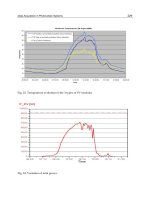
Fig. 23. Temperature evolution of the 3 types of PV modules





Fig. 24. Variation of total power

Renewable Energy – Trends and Applications

230
5. Conclusion
Even though the costs of installations producing electric energy with PV panels are high
compared to the costs of conventional installations, the number of such systems is
continuously increasing. It is very important to determine the output characteristics of the
PV panels in order to achieve an accurate connection and operation of the device and reduce
energy losses.
Monitoring activities follow the operation analysis by periodical reports, papers, synthesis,
with the precise aim to make the most accurate decisions to produce electric energy using
unconventional sources.
To quantify the potential for performance improvement of a PV system, data acquisition
systems has been installed. The importance of this chapter consists in the presentation of a

dedicated DAQ used in PV system analysis and real data measurements. The operation is
performed by simulations using LabVIEW™.
The information obtained by monitoring parameters, such as voltage, current, power and
energies are fed to the PC via the DAQ for analysis. The control interface has been
developed by utilizing LabVIEW™ software. The system has been in operation during the
last five years and all its units have functioned well.
6. References
Andrei, H.; Dogaru, V.; Chicco, G.; Cepisca, C. & Spertino, F. (2007). Photovoltaic
Applications, Journal of Materials Processing Technology, 181 (1-3), 2007, 267-273
Andrei, H.; Cepisca, C.; Grigorescu, SD.; Ivanovici, T. & Andrei, P. (2010). Modeling of the
PV panels circuit parameters using the 4 - terminals equations and Brune’s
conditions, Scientific Bulletin of the Electrical Engineering Faculty, 10 (1), 2010, 63-67
Ambros, T., et.al. (2004). Renewable energy, TEHNICA-INFO, Kishinev
Awerbuch, S. (2002). Energy Diversity and Security in the EU: Mean -Variance Portfolio
Analysis of Electricity Generating Mixes, and the Implications for Renewable Sources,
Proceedings of EURELECTRIC Twin Conf. on DG, pp. 120-125, Brussels, Belgium, 2002
Cepisca, C.; Andrei, H.; Dogaru Ulieru,V. & Ivanovici, T. (2004). Simulation and data
acquisition of the photovoltaic systems using LabVIEW™, Proceedings of ICL 2004,
pp. 80-84, Villach, Austria, 2004
Dogaru Ulieru,V.; Cepisca, C. & Ivanovici, T. (2009). Data Acquisition in Photovoltaic
Systems, Proceedings of 13
th
WSEAS International Conference on Circuits, Systems,
Communications and Computers, pp. 234-238, Rodos Island, Greece, July 22-24, 2009
Ertugrul, N. (2002). LabVIEW™ for electric circuits, machines, drives and laboratories, Ed.
Prentice Hall, New York
Judd,B. (2008). Everything You Ever Wanted to Know about Data Acquisition, In: United
Electronic Industries, 2008, available from www.ueidaq.com
Manea,F. & Cepisca, C. (2007). PHP+Apache+Testpoint -An original way for having remote
control over any type of automation, Scientific Bulletin UPB, Series C Electrical

Engineering, 69 (2), 2007, 85-92
Nawrocki, W. (2005). Measurement System and Sensors, Artech House, London
Szekely, I. (1997). Systems for data acquisition and processing, Ed. Mediamira, Cluj–Napoca
Vasile, N. (2009). Players on the market in renewable energy, Round Table - renewable sources of
energy between the European Directive 77/2001 and reality, Bucharest, Romania, May 2009
11
Optimum Design of a Hybrid
Renewable Energy System
Fatemeh Jahanbani and Gholam H. Riahy
Electrical Engineering Department, Amirkabir University of Technology
Iran
1. Introduction
In Iran, 100% of the region populated with more than 20 families is electrified. For the other
regions the electrification will be done. These regions almost are rural and remote areas. For
utility company it is important that electrification be done with the least cost.
Many alternative solutions could be used for this goal (decreasing the cost). Using
renewable energy system is one of the possible solutions. A growing interest in renewable
energy resources has been observed for several years, due to their pollution free energy,
availability, and continuity. In practice, use of hybrid energy systems can be a viable way to
achieve trade-off solutions in terms of costs. Photovoltaic (PV) and wind generation (WG)
units are the most promising technologies for supplying load in remote and rural regions
[Wang et al., 2007]. Therefore, in order to satisfy the load demand, hybrid energy systems
are implemented to combine solar and wind energy units and to mitigate or even cancel out
the power fluctuations. Energy storage technologies, such as storage batteries (SBs) can be
employed. The proper size of storage system is site specific and depends on the amount of
renewable energy generation and the load.
Many papers are discussed on design of hybrid systems with the different components.
Also, various optimization techniques are used by researchers to design hybrid energy
system in the most cost effective way.
Rahman and Chedid give the concept of the optimal design of a hybrid wind–solar power

system with battery storage and diesel sets. They developed linear programming model to
minimize the average production cost of electricity while meeting the load requirements in a
reliable manner, and takes environmental factors into consideration both in the design and
operation phases [Chedid et al., 1997]. In [Kellogg et al, 1996], authors proposed an iterative
technique to find the optimal unit sizing of a stand-alone and connected system. In 2006 is
presented a methodology for optimal sizing of stand-alone PV/WG systems using genetic
algorithms. They applied design approach of a power generation system, which supplies a
residential household [Koutroulis et al, 2006]. In [Ekren, 2008], authors used the response
surface methodology (RSM) in size optimization of an autonomous PV/wind integrated
hybrid energy system with battery storage. In [Shahirinia, 2005], an optimized design of
stand-alone multi sources power system includes sources like, wind farm, photovoltaic
array, diesel generator, and battery bank based on a genetic algorithm is presented. Also,
authors in [Koutroulis et al, 2006, Tina, 2006] used multi-objective genetic algorithm, in

Renewable Energy – Trends and Applications

232
order to calculate reliability/cost implications of hybrid PV/wind energy system in small
isolated power systems. Yang developed a novel optimization sizing model for hybrid
solar–wind power generation system [Yang et al., 2007]. In [Terra, 2006] an automatic multi-
objective optimization procedure base on fuzzy logic for grid connected HSWPS design is
described. In some later works, PSO is successfully implemented for optimal sizing of
hybrid stand-alone power systems, assuming continuous and reliable supply of the load
[Lopez, 2008, Belfkira, 2008]. Karki and Billinton presented a Monte-Carlo simulation
approach to calculate the reliability index [Karki et al., 2001] and Kashefi presented a
method for assessment of reliability basis on binominal distribution function for hybrid
PV/wind/fuel cell energy system that is used in this study [Wang et al., 2007].
As previous studies shown, renewable energies are going to be a main substitute for fossil
fuels in the coming years for their clean and renewable nature [Sarhaddi et al., 2010].
Photovoltaic solar and wind energy conversion systems have been widely used for

electricity supply in isolated locations that are far from the distribution network.
The future of power grids is expected to involve an increasing level of intelligence and
integration of new information and communication technologies in every aspect of the
electricity system, from demand-side devices to wide-scale distributed generation to a
variety of energy markets.
In the smart grid, energy from diverse sources is combined to serve customer needs while
minimizing the impact on the environment and maximizing sustainability. In addition to
nuclear, coal, hydroelectric, oil, and gas-based generation, energy will come from solar,
wind, biomass, tidal, and other renewable sources. The smart grid will support not only
centralized, large-scale power plants and energy farms but residential-scale dispersed
distributed energy sources [Santacana et al., 2010].
Being able to accommodate distributed generation is an important characteristic of the smart
grid. Because of mandated renewable portfolio standards, net metering requirements and a
desire by some consumers to be green, there is an increasing need to be prepared to be able
to interconnect generation to distribution systems, especially renewable generation such as
photovoltaic, small wind and land fill gas powered generation [Saint, 2009].
The future electric grid will invariably feature rapid integration of alternative forms for energy
generation. As a national priority, renewable energy resources applications to offset the
dependence on fossil fuels provide green power options for atmospheric emissions
curtailment and provision of peak load shaving are being put in policy [Santacana et al., 2010].
Fortunately, Iran is a country with the adequate average of solar radiation and wind speed
for setting up a hybrid power generation e.g. the average of wind speed and perpendicular
solar radiation were recorded for Ardebil province is 5.5945 m/s and 203.1629 W/m
2

respectively in a year.
In this study, an optimal hybrid energy generation system including of wind, photovoltaic
and battery is designed. The aim of design is to minimize the cost of the stand-alone system
over its 20 years of operation. The optimization problem is subject to economic and technical
constraints. Figure1 show the framework of activities in this study.

The generated power by wind turbine and PV arrays are depended on many parameters
that the most effectual of them are wind speed, the height of WTs hub (that affects the wind
speed), solar radiations and orientation of PV panels. In certain region, the optimization
variables are considered as the number of WTs, number of PV arrays, installation angle of
PV arrays, number of storage batteries, height of the hub and sizes of DC/AC converter. The

Optimum Design of a Hybrid Renewable Energy System

233
goal of this study is optimal design of hybrid system for the North West of Iran (Ardebil
province). The data of hourly wind speed, hourly vertical and horizontal solar radiation and
load during a year are measured in the region. This region is located in north-west of Iran
and there are some villages far from the national grid. The optimization is carried out by
Particle Swarm Optimization (PSO) algorithm. The objective function is cost with
considered economical and technical constraints. Three different scenarios are considered
and finally economical system is selected.


Fig. 1. The framework of activities
This study is organized as follows: section 2 describes the modeling of system components.
The reliability assessment is discussed in section 3. Problem formulation and operation
strategy are explained in section 4 and 5, respectively. In the next section, is dedicated to
particle swarm optimization. Simulation and results are summarized in section 7. Finally,
section 8 is devoted to conclusion.
2. Description of the hybrid system
The increasing energy demand and environmental concerns aroused considerable interest in
hybrid renewable energy systems and its subsequent development.
The generation of both wind power and solar power is very dependent on the weather
conditions. Thus, no single source of energy is capable of supplying cost-effective and
reliable power. The combined use of multiple power resources can be a viable way to

achieve trade-off solutions. With combine of the renewable systems, it is possible that power
fluctuations will be incurred. To mitigate or even cancel out the fluctuations, energy storage
technologies, such as storage batteries (SBs) can be employed [Wang et al., 2009].
The proper size of storage system is site specific and depends on the amount of renewable
generation and the load. The needed storage capacity can be reduced to a minimum when a
proper combination of wind and solar generation is used for a given site [Kellogg, 1996].
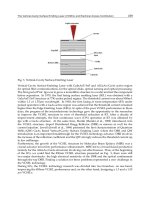
The hybrid system is shown in Fig. 2. In the following sections, the model of components is
discussed.

Renewable Energy – Trends and Applications

234

Fig. 2. Block diagram of a hybrid wind/photovoltaic generation unit
2.1 The wind turbine
Choosing a suitable model is very important for wind turbine power output simulations.
The most simplified model to simulate the power output of a wind turbine could be
calculated from its power-speed curve. This curve is given by manufacturer and usually
describes the real power transferred from WG to DC bus.
The model of WG is considered BWC Excel-R/48 (see Fig. 3) [Hakimi et al., 2009]. It has a
rated capacity of 7.5 kW and provides 48 V dc as output. The power of wind turbine is
described in terms of the wind speed according to Eq. 1.


Fig. 3. Power output characteristic of BWC Excel R/48 versus wind speed [Hakimi, 2009].


max
max
max

0,
WciWco
m
Wci
WW ciWr
rci
fW
WWrrWf
co r
vvvv
vv
PP vvv
vv
PP
Pvvvvv
vv








 













(1)

Optimum Design of a Hybrid Renewable Energy System

235
where
max
WG
P ,
f
P are WG output power at rated and cut-out speeds, respectively. Also,
r
v ,
ci
v ,
co
v are rated, cut-in and cut-out wind speeds, respectively. In this study, the exponent m
is considered 3. In the above equation,
W
v refers to wind speed at the height of WG’s hub.
Since,
W
v almost is measured at any height (here, 40 m), not in height of WGs hub, is used Eq.

(2) to convert wind speed to installation height through power law [Borowy et al., 1996]:

measure
hub
WW
measure
h
vv
h





(2)
where α is the exponent law coefficient. α varies with such parameters as elevation, time of
day, season, nature of terrain, wind speed, temperature, and various thermal and
mechanical mixing parameters. The determination of α becomes very important. The value
of 0.14 is usually taken when there is no specific site data (as here) [Yang et al., 2007].
2.2 The photovoltaic arrays (PVs)
Solar energy is one of the most significant renewable energy sources that world needs. The
major applications of solar energy can be classified into two categories: solar thermal
system, which converts solar energy to thermal energy, and photovoltaic (PV) system,
which converts solar energy to electrical energy. In the following, the modeling of PV arrays
is described.
For calculating the output electric power of PVs, perpendicular radiation is needed. When
the hourly horizontal and vertical solar radiation is available (as this study), perpendicular
radiation can be calculated by Eq. (3):












,cos sin
PV V PV H PV
Gt G t G t

  (3)
where,

V
Gt and


H
Gt are the rate of vertical and horizontal radiations in the t
th
step-
time (W/m
2
), respectively. The radiated solar power on the surface of each PV array can be
calculated by Eq. (4):

,

1000
p
v
p
vrated MPPT
G
PP

 
(4)
where, G is perpendicular radiation at the arrays’ surface (W/m
2
).
,
p
vrated
P is rated power of
each PV array at
2
1000( / )GWm and
M
PPT

is the efficiency of PV’s DC/DC converter
and Maximum Power Point Tracking (MPPT).
2.3 The storage batteries
Since both wind and PVs are intermediate sources of power, it is highly desirable to
incorporate energy storage into such hybrid power systems. Energy storage can smooth out
the fluctuation of wind and solar power and improve the load availability [Borowy et al.,
1996].

When the power generated by WGs and PVs are greater than the load demand, the surplus
power will be stored in the storage batteries for future use. On the contrary, when there is
any deficiency in the power generation of renewable sources, the stored power will be used
to supply the load. This will enhance the system reliability.

Renewable Energy – Trends and Applications

236
In the state of charge, amount of energy that will be stored in batteries at time step of t is
calculated:

  


 


.
1/
BB w
p
v Load inv Bat
Et Et P P t P t


  (5)
In addition, Eq. 6 will calculate the state of battery discharge at time step of t:

   






.
1/
BB Loadinvw
p
vBat
Et Et P t P P t


  (6)
where,

B
Et
,


1
B
Et

are the stored energy of battery in time step of t and (t-1).
w
P ,
p
v
P

are the generated power by wind turbines and PV arrays,


Load
Pt
is the load demand at
time step of t and
Bat

is the efficiency of storage batteries.
2.4 The power inverter
The power electronic circuit (inverter) used to convert DC into AC form at the desired
frequency of the load. The DC input to the inverter can be from any of the following sources:
1.
DC output of the variable speed wind power system
2.
DC output of the PV power system
In this study, supposed the inverter’s efficiency is constant for whole working range of
inverter (here 0.9).
3. The reliability assessment
A widely accepted definition of reliability is as follows [Billinton, 1992]: “Reliability is the
probability of a device performing its purpose adequately for the period of time intended
under the operating conditions encountered”. In the following sections, reliability indices
and reliability model that is used in this study is described.
3.1 Reliability indices
Several reliability indices are introduced in literature [Billinton, 1994, XU et al., 2005]. Some of
the most common used indices in the reliability evaluation of generating systems are Loss of
Load Expected (LOLE), Loss of Energy Expected (LOEE) or Expected Energy not Supplied
(EENS), Loss of Power Supply Probability (LPSP) and Equivalent Loss Factor (ELF).
In this study, ELF is chosen as the main reliability index. On the other word, the ELF index

is chosen as a constraint that must be satisfied but it could be possible to calculate the other
indexes as is done in this study (such as EENS, LOLE and LOEE indexes).
ELF is ratio of effective load outage hours to the total number of hours. It contains
information about both the number and magnitude of outages. In the rural areas and stand-
alone applications (as this study), ELF<0.01 is acceptable. Electricity supplier aim at 0.0001
in developed countries [Garcia et al., 2006]:

1
1(())
()
H
h
EQh
ELF
HDh



(7)
where,
Q(h) and D(h) are the amount of load that is not satisfied and demand power in h
th

step, respectively and
H is the number of time steps (here H=8760).

Optimum Design of a Hybrid Renewable Energy System

237
In this study, the reliability index is calculated from component’s failure, that is concluding

of wind turbine, PV array, and inverter failure.
3.2 System’s reliability model
As mentioned, outages of PV arrays, wind turbine generators, and DC/AC converter are
taken into consideration. Forced outage rate (FOR) of PVs and WGs is assumed to be 4%
[Karki et al., 2001]. So, these components will be available with a probability of 96%.
Probability of encountering each state is calculated by binomial distribution function
[Nomura 2005].
For example, given
n
WG
fail out of total N
WG
installed WGs, and n
PV
fail out of total N
PV

installed PV arrays are failed, the probability of encountering this state is calculated as
follows:


 
,1 1
fail fail
fail fail
WG PV
WG PV
PV
WG PV
WG PV

fail
fail
Nn Nn
nn
fail fail
WG
ren WG PV
PV
WG
WG
PV
n
n
fnn A A A A
N
N









     













(8)
The outage probability of other components is negligible. But, because, DC/AC converter is
the only single cut-set of the system reliability diagram, the outage probability of it is taken
consideration (it’s FOR is considered 0.0011 [Kashefi et al., 2009]).
In [Kashefi et al., 2009] an approximate method is used that proposed all the possible states
for outages of WGs and PV arrays to be modeled with an equivalent state. This idea is
modeled by Eq. 7.



ren WG WG WG PV PV PV
EP N P A N P A
(9)
4. Problem formulation
The economical viability of a proposed plant is influence by several factors that contribute to
the expected profitability. In the economical analysis, the system costs are involved as:
-
Capital cost of each component
-
Replacement cost of each component
-
Operation and maintenance cost of each component

-
Cost costumer’s dissatisfaction
It is desirable that the system meets the electrical demand, the costs are minimized and the
components have optimal sizes. Optimization variables are number of WGs, number of PV
arrays, installation angle of PV arrays, number of storage batteries, and sizes of DC/AC
converter. For calculation of system cost, the Net Present Cost (NPC) is chosen.
For optimal design of a hybrid system, total costs are defined as follow:



(&1/,)
ii i ii i
NPC N CC RC K O MC CRF ir R    (10)
where
N may be number (unit) or capacity (kW), CC is capital cost (US$/unit), O&MC is
annual operation and maintenance cost (US$/unit-yr) of the component.
R is Life span of
project,
ir is the real interest rate (6%). CRF and K are capital recovery factor and single
payment present worth, respectively.

Renewable Energy – Trends and Applications

238




1
nominal

ir
f
ir
f



(11)




1
,
11
R
R
ir ir
CRF ir R
ir




(12)


1
1
1

i
i
y
i
nL
n
K
ir





(13)
4.1 The cost of loss of load
In this study, cost of electricity interruptions is considered. The values found for this
parameter are in the range of 5-40 US$/kWh for industrial users and 2-12 US$/kWh for
domestic users [Garcia et al., 2006]. In this study, the cost of customer’s dissatisfaction,
caused by loss of load, is assumed to be 5.6 US$/kWh [Garcia et al., 2006].
Annual cost of loss of load is calculated by:

loss loss
NPC LOEE C PWA

 (14)
where,
loss
C is cost of costumer’s dissatisfaction (in this study, US$5.6/kWh). Now, the
objective function with aim to minimize total cost of system is described:

iloss
i
Cost NPC NPC

(15)
where
i indicates type of the source, wind, PV, or battery. To solve the optimization
problem, all the below constraints have to be considered:


min max
max
&
max
0
10 20
0
2
i
hub
PV PVT
bat bat bat
NN
H
EEE
EELF ELF








(16)
The last constraint is the reliability constraint. Equivalent Loss Factor is ratio of effective
load outage hours to the total number of hours. In the rural areas and stand-alone
applications (as this study), ELF<0.01 is acceptable [Tina, 2006]. For solving the optimization
problem, particle swarm algorithm has been exploited.
5. Operation strategy
The system is simulated for each hour in period of one year. In each step time, one of the
below states can occur:
-
If the total power generated by PV arrays and WGs are greater than demanded load,
the energy surplus is stored in the batteries until the full energy is stored. The
remainder of the available power is consumed in the dump load.

Optimum Design of a Hybrid Renewable Energy System

239
- If the total power generated by PV arrays and WGs are less than demanded load,
shortage power would be provided from batteries. If batteries could not provide total
energy that loads demanded, the load will be cut.
-
If the total power generated by PV arrays and WGs are equal to the demanded load, the
storage capacity remains unchanged and all of the generated power will be consumed
at the load.
By consideration these states and all the constraints, the optimal hybrid system is calculated.
6. Optimization method
For size optimization of components PSO algorithm is used. Direct search method
(traditional optimization method) heavily depends on good starting points, and may fall

into local optima. On the other hand, as a global method for solving both constrained and
unconstrained optimization problems based on natural evolution, the PSO can be applied to
solve a variety of optimization problems that are not well suited for standard optimization
algorithms. Moreover, the GA can also be employed to solve a variety of optimization
problems. Compared to GA, the advantages of PSO are that PSO is easy to implement and
there are few parameters to adjust. PSO has been successfully applied in many areas.
6.1 The PSO algorithm
Particle swarm optimization was introduced in 1995 by Kennedy and Eberhart. The
following is a brief introduction to the operation of the PSO algorithm. The particle swarm
optimization (PSO) algorithm is a member of the wide category of swarm intelligence
methods for solving global optimization problems. PSO is an evolutionary algorithm
technique through individual improvement plus population cooperation and competition
which is based on the simulation of simplified social models, such as bird flocking, fish
schooling and the swarm theory [Jahanbani et al., 2008].
Each individual in PSO, referred as a particle, represents a potential solution. In analogy
with evolutionary computation paradigms, a swarm is similar to population, while a
particle is similar to an individual.
In simple terms, each particle is flown through a multidimensional search space, where the
position of each particle is adjusted according to its own experience and that of its
neighbors.
Assume
x and v denote a particle position and its speed in the search space. Therefore, the
i
th
particle can be represented as
12
[ , , , , , ]
dN
iii i i
xxxxx


in the N-dimensional space. Each
particle continuously records the best solution it has achieved thus far during its flight. This
fitness value of the solution is called pbest. The best previous position of the i
th
particle is
memorized and represented as:

12
[ , , , , , ]
dN
iiiii
p
best
p
best
p
best
p
best
p
best

(17)
The global best
gbest is also tracked by the optimizer, which is the best value achieved so far
by any particle in the swarm. The best particle of all the particles in the swarm is denoted by
gbest
d
. The velocity for particle i is represented as

12
[ , , , , , ]
dN
iii i i
vvvvv

.
The velocity and position of each particle can be continuously adjusted based on the current
velocity and the distance from
pbest
id
to gbest
d
:

Renewable Energy – Trends and Applications

240

11 22
( 1) () () ( () ()) ( () ())
iiii
vt tvt crPt Xt crGt Xt


(18)

(1) () (1)
iii
Xt Xt vt



 
(19)
where
c
1
and c
2
are acceleration constants and r
1
and r
2
are random real numbers drawn
from [0,1]. Thus the particle flies trough potential solutions toward ()
i
Pt and ()Gt in a
navigated way while still exploring new areas by the stochastic mechanism to escape from
local optima.
Since there was no actual mechanism for controlling the velocity of a particle, it was
necessary to impose a maximum value
V
max
, which controls the maximum travel distance in
each iteration to avoid this particle flying past good solutions. Also after updating the
positions, it must be checked that no particle violates the boundaries of search space. If a
particle has violated the boundaries, it will be set at boundary of search space [Jahanbani et
al., 2008].
In Eq. (20),
()t


is employed to control the impact of the previous history of velocities on
the current one and is extremely important to ensure convergent behavior. It is exposed
completely in the following section. ()t

is the constriction coefficient, which is used to
restrain velocity.

is constriction factor which is used to limit velocity, here 0.7

 .
7. Simulation results
The first goal of each planning in electrical network is that the system meets the demand.
For satisfying this goal, the cost of costumer’s dissatisfaction is considered as well as the
other costs. Flowchart of the proposed optimization methodology is shown in Fig. 4. The
hourly data of wind speed, vertical and horizontal solar radiation and residential load
during a year is plotted in Fig. 5, Fig. 6 and Fig. 7, respectively. The data that used in this
study is the data of Ardebil convince that is located in the North West of Iran (latitude:
38°17´, longitude: 48°15´, altitude: 1345 m). The peak load is considered as 50 kW. In table 1,
data that used in the simulation are listed.


Fig. 4. Flowchart of the proposed optimization methodology.

Optimum Design of a Hybrid Renewable Energy System

241
System parameters values System parameters values
Efficiency of SB 85%
Replacement price of PV

array
6000 US$/unit
Efficiency of inverter 90% Replacement price of SB 700 US$/unit
Life span of project 20
Replacement price of
inverter
750 US$/unit
Life span of WTG and PV 20 OM costs of inverter 8 US$/unit-yr
Life span of SB 10 Cut-in wind speed 3 m/s
Life span of inverter 15 Rated wind speed 13 m/s
PV array price 7000 US$/unit Cut-out wind speed 25 m/s
WTG price
19400
US$/unit
Rated WTG power 7.5 kW
Inverter price 800 US$/unit
Minimum storage level of
battery
3 kWh
Replacement price of
WTG
15000
US$/unit
Maximum total SB capacity 40 kWh
Table 1. Data used for simulation program [Tina et al., 2006, Khan et al., 2005]

0 1000 2000 3000 4000 5000 6000 7000 8000 9000
0
5
10

15
20
25
Time (hour)
Annual wind speed (m/s)

Fig. 5. Hourly wind speed during a year.

Renewable Energy – Trends and Applications

242
0 1000 2000 3000 4000 5000 6000 7000 8000
0
200
400
600
800
1000
Time (hour)
Annual radiation (W/m
2
)


Vertical
Horizontal

Fig. 6. Hourly vertical and horizontal solar radiation during a year.

0 1000 2000 3000 4000 5000 6000 7000 8000 9000

10
15
20
25
30
35
40
45
50
Time (hour)
Load power (kW)

Fig. 7. Hourly residential load during a year.
It is noticeable that the technical constraint, related to system reliability, is expressed by the
equivalent loss factor. The reliability index is calculated from component’s failure, that
includes wind turbine, PV array, battery and inverter failure. The power generated by each
wind turbine and PV array can be derived by Eq. (1) and Eq. (3), respectively. The total
power that can be generated with N
WG
wind turbines and N
PV
PV arrays that n
WG
and n
PV
of
all wind turbines and PV arrays are out of work, respectively, will be calculated as follows:

() ()
ren WG WG WG WG PV PV PV PV

PNn APNnAP
(20)

Optimum Design of a Hybrid Renewable Energy System

243
As previously mentioned, the reliability constraint is considered as the penalty factor in the
objective function. To consider the constraint of reliability in Eq. (16), the excess amount of
inequality constraint is multiplied by 1010 and then, this additional cost is added to the
objective function in Eq. (15). With this method, the NPC of the system that couldn't satisfy
the reliability constraint will increase, and then this system would not be chosen as the best
economic system.
One of the best methods in the planning area is using scenario method. To choose the best
plan (the minimum cost) different scenarios is implemented. In this study, the
optimal size
of components for hybrid system is calculated in three scenarios based on proposed
approach. These systems are PV/battery system, wind/battery system and
PV/wind/battery system. For each system the minimum cost and reliability indices is
calculated. The results are shown in the following.
As mentioned before, in this study particle swarm optimization algorithm is used for optimal
sizing of system’s components. Each particle has 6 variables that are defined as below:

Number of
wind turbine

Number of
PV array

Angle of PV
Battery

capacity

Height of hub
Inverter
capacity

Fig. 8. A typical vector for a particle
Each population consists of 30 particles that are calculated for 120 iterations. The fitness
function is defined in Eq. (15). It must be considered that if the costs of loss of load are more
expensive than the cost of bigger system, the bigger system will be chosen because it is
economically reasonable.
7.1 Scenario I: Wind/PV/battery hybrid system
In this case, a stand-alone hybrid system is considered that is including of wind and PV
energy sources and storage batteries. Convergence curves of the PSO algorithm, for five
independent runs, are shown in Fig. 9. It is observed that the algorithm converges almost to
the same optimal value.
Hourly generated power of PV arrays, WGs is shown in Fig. 10 that could be comparing
with load. The hourly expected amount of stored energy in the battery is shown in Fig.
10, too. It is significant that reliable supply of the load at each time step, strongly,
depends on the amount of the stored energy. When stored energy in battery reaches its
minimum allowable limit, if renewable system cannot satisfy the load, the load will not
be supplied. On the other hand, if renewable system can satisfy the load, the extra
generated energy will be saved in the battery (and battery is in the state of charge). It is
worth pointing out that when the battery has the maximum charge its energy will not
increase anymore.
In Fig. 11, the hourly reliability indices in the year are plotted. The amount of hourly
demand and load pattern is another important factor in reliability assessment of the system.
The size of each component is also calculated and is shown in table 2.
As shown in the above figures, each time step could be analyzed. For example, at around of
6500

th
time step, the power that is generated by PV arrays and wind turbines is decreased
(Fig. 10) and it is not enough to satisfy the load. Also, the energy that saved in the batteries
in this step is around the minimum allowable level. So, some of the demand is lost and ELF
index is equal to 0.5 (Fig. 11).

Renewable Energy – Trends and Applications

244






0 20 40 60 80 100 120
0.6
0.8
1
1.2
1.4
1.6
1.8
2
2.2
2.4
2.6
x 1
0
6

Number of iteration
Total cost (US$)






Fig. 9. Convergence of the optimization algorithm

N
WG
N
PV
N
Ba
t
P
inv
(kW) θ
PV
H
hub
(m)
1 89 12 44 52.61 15.85

Table 2. Optimal combination for hybrid system

ELF LOEE (kWh/yr) EENS LOLE(h/yr)
0.0036 759.49 0.0034 64.57

Table 3. Reliability indices of PV-wind-battery system

Optimum Design of a Hybrid Renewable Energy System

245









0 1000 2000 3000 4000 5000 6000 7000 8000
0
20
40
60
Load power (kW)
0 1000 2000 3000 4000 5000 6000 7000 8000
0
5
10
Wind power
generation (kW)
0 1000 2000 3000 4000 5000 6000 7000 8000
0
50

100
PV power
generation (kW)
0 1000 2000 3000 4000 5000 6000 7000 8000
0
200
400
600
Time (hour)
Battery energy (kWh)










Fig. 10. Hourly generated power of PV arrays, WGs and hourly expected amount of stored
energy in the battery during a year.

Renewable Energy – Trends and Applications

246

0 1000 2000 3000 4000 5000 6000 7000 8000
0
0.5
1
ELF
0 1000 2000 3000 4000 5000 6000 7000 8000
0
0.5
1
LOLE
0 1000 2000 3000 4000 5000 6000 7000 8000
0
10
20
30
LOEE (kWh)
Time (hour)






Fig. 11. Hourly reliability indices during a year
In this scenario, the mean of ELF index in the year is 0.002 which is less than the maximum
ELF tconstraint (0.01). So, this system would not pay for penalty cost. The NPC, which is
calculated for this case, would be equal to 1.29769 MUSD that 31272.02 USD of this cost
would be for costumer’s dissatisfaction.
7.2 Scenario II: Wind/battery system

This system is including of wind source energy and storage batteries. The optimal size of
system components is presented in table 4. In this case, the reliability constraint is activated,
so it is fixed on maximum allowable value. Because of this, the NPC of system is increased
and is reached up to 2.25009 MUS$. The generated power by wind turbines and amount of
energy in storage system is shown in Fig. 12.
As mentioned, in this system, the ELF index is reached to 0.0063 which satisfy the inequality
constraint of reliability constraint. Thus, it must not pay the penalty cost and the costumer’s
dissatisfaction cost would be 0.032424 MUS$.

Optimum Design of a Hybrid Renewable Energy System

247
0 1000 2000 3000 4000 5000 6000 7000 8000
10
20
30
40
50
Load power (kW)
0 1000 2000 3000 4000 5000 6000 7000 8000
0
200
400
600
800
Wind power
generation (kW)
0 1000 2000 3000 4000 5000 6000 7000 8000
0
2000

4000
6000
8000
10000
Time (hour)
Battery energy (kWh)

Fig. 12. Hourly generated power of WGs and hourly expected amount of stored energy in
the battery during a year.

N
WG
N
PV
N
Ba
t
P
inv
(kW) θ
PV
H
hub
(m)
80 - 230 44.5 - 19
Table 4. Optimal combination in wind-Battery system

ELF LOEE (kWh/yr) EENS LOLE(h/yr)
0.0063 1315.6 0.0063 77.56
Table 5. Reliability indices of wind-battery system

7.3 Scenario III: PV/Battery systems
The last scenario is a system including of PV source energy and storage batteries. The size of
system components is shown in table 6. Total cost and ELF index corresponding to this case
are 0.803237 MUS$ and 0.0022 respectively that, 0.032423 MUS$ would be paid as
costumer’s dissatisfaction cost. The output power of PV arrays and battery energy is shown
in Fig. 13.

Renewable Energy – Trends and Applications

248
0 1000 2000 3000 4000 5000 6000 7000 8000
10
20
30
40
50
Load power (kW)
0 1000 2000 3000 4000 5000 6000 7000 8000
0
20
40
60
80
100
PV power generation (kW)
0 1000 2000 3000 4000 5000 6000 7000 8000
0
200
400
600

Time (hour)
Battery energy (kWh)

Fig. 13. Hourly generated power of PV arrays and hourly expected amount of stored energy
in the battery during a year.

N
WG
N
PV
N
Ba
t
P
inv
(kW) θ
PV
H
hub
(m)
- 96 13 44.3 56.74 11
Table 6. Optimal combination in PV-battery system

ELF LOEE (kWh/yr) EENS LOLE(h/yr)
0.0022 504.79 0.0024 49.59
Table 7. Reliability indices of PV-battery system
With compare of these scenarios together, it could be seen, the number of batteries in wind-
battery system is more than the hybrid system and PV-battery system. That’s reasonable
because in this region (and almost all of regions) fluctuations of wind are more than the
fluctuations in radiation, so, when the wind turbine is used, we needed to add more storage

system to be sure that the load would be met in all steps. Also, in this region, the peak load
is nearer to the peak of PV generation compared with the peak of wind generation. On the