Emerging Communications for Wireless Sensor Networks Part 7 ppt

A new MAC Approach in Wireless Body Sensor Networks for Health Care 113

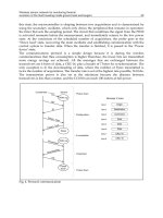
practically speaking, each body sensor access request could be a separate modulated signal
transmission (Xu & Campbell, 1992). Similarly, for the DQBAN novel n scheduling minislots,
the same length of 1 byte is reserved to indicate either forward or delay (i.e. Decision output
linguistic values). In our current DQBAN simulations, there are m = 3 access minislots (as in
the original (Xu & Campbell, 1992); and n = 5 scheduling minislots, even though n could be
configurable from DQBAN superframe to DQBAN superframe, depending on the number
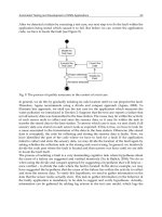
of body sensors in DTQ. To simulate the fuzzy-logic system integrated each body sensor, we
utilize a MATLAB fuzz-logic toolbox. The aforementioned


1 3
X , X
values for each
membership function (see Fig 8) are derived by computer simulations as: (a)
   
1 3
X , X 1.8,12.8
dB for SNR (following Table 3); (b)




1 3
X ,X -0.108,0.012
seconds for
WT, and (c)
 



1 3
X , X 1000, 2000
mAh for BL.

8.2 Simulation results
For the overall evaluation of the DQBAN MAC system performance, we carried out the
following models and comparisons among them in both homogenous and heterogeneous
depicted hospital care scenarios,
A. DQBAN model (i.e. with the fuzzy-logic system scheduler and energy-aware radio
activation policies),
B. DQ model with a general cost function scheduler as in (Chen et al., 2006) and energy-
aware radio activation policies,
C. DQ without any scheduler implementation as in Section 4 (i.e. though with the energy-
aware radio activation policies),
D. DQ with neither any energy-aware radio activation policy nor any scheduling algorithm
implementation, that is as in (Lin & Campbell, 1993); (Xu & Campbell, 1992).

The results of the “Delivery Ratio”, “Mean Packet Delay” and “Average Energy
Consumption per Utile Bit” metrics are portrayed in Fig. 9 and Fig. 10 after long iterating
and achieving the permanent regime of the DQBAN scheme.

Homogenous Scenario
Fig. 10 depicts the DQBAN MAC performance in a homogenous BSN with an increasing
number of 1-lead ECG body sensors, whose characteristics are specified in Table 2. Note that
20% of the ECG sensors involved in each simulation are initially charged with much less
amount of battery. The idea is to evaluate the energy-saving behavior of the DQBAN system
as the traffic load rises until saturation conditions. The “Average Energy Consumption per
Utile Bit” in graphic Fig. 10(a) illustrates the requirement of an energy-aware activation
policy. In a typical DQ MAC protocol (Lin & Campbell, 1993); (Xu & Campbell, 1992), no
energy-saving techniques are utilized. Therefore, as the traffic load increases in the BSN,

body sensors remaining longer in the system may run out of battery. As a result, the average
energy-consumption per delivered information bit increases. Fig. 10(c) emphasizes that by
using energy-aware radio activation policies plus a scheduling algorithm, the MAC layer
improves in terms of average energy consumption per utile bit. DQBAN outperforms the
aforementioned B. and C. implementations. Notice that it was already proved in Section 4
that the energy-consumption of the DQ MAC (implementation C.) outperforms 802.15.4 in

all possible scenarios. The “Delivery Ratio” graphic Fig. 10(b) proves that the fact of
scheduling data packets taking cross-layer constraints into account outperforms the first
come first served discipline of the original DQ protocol by guaranteeing the QoS
requirements of high reliability, right message latency and enough battery lifetime to all
body sensors transmissions in the BSN (as described in Section 7.2). The use of DQBAN with
the proposed cross-layer fuzzy-rule base scheduling algorithm reaches more than 95% of
transmission successes, even though 20% of the ECG sensors have critical battery
constraints. Close to saturation limits, DQBAN achievement is specifically 42.75% superior
to the original DQ protocol without any energy-aware policy (i.e. implementation D.) and
11.78% superior compared to implementation C. The slight raise in the “Delivery Ratio”, in
implementations A. and B., results from the growing number of body sensors in DTQ. That
is, it is easier to find a body sensor with the appropriate environmental conditions to be
scheduled in the first place, while others are reluctant to transmit. Further, Fig. 10(d)
confirms that the use DQBAN is also appropriate in terms of “Mean Packet Delay” and still
outperforms implementation B., as in all previous studied scenarios.

Fig. 10. “Average energy consumption per utile bit” (a) – (c), “Delivery Ratio” (b) and
“Mean Packet Delay” (d) in the homogenous Scenario


Emerging Communications for Wireless Sensor Networks114

Heterogeneous Scenario

Fig. 11 illustrates the DQBAN MAC performance in a hospital scenario with heterogeneous
traffic. The heterogeneous BSN is characterized by four specific medical body/portable
sensors defined in Table 2; a blood pressure body sensor, a respiratory rate body sensor, a
real-time endoscope camera and a portable clinical PDA, while the number of ECG body
sensors increases from simulated iteration to iteration, as previously explained. In order to
facilitate the evaluation of the “Delivery Ratio” metric of the implementations A., B. and C.,
Fig. 11(a) portrays the performance of the Blood Pressure body sensor and the average
performance of the total number of ECG sensors in the heterogeneous BSN, separately. When
it comes to evaluate the “Delivery Ratio” of the Blood Pressure body sensor, DQBAN is
specifically 3.44% and 10% higher than that of implementations B. and C., respectively. In
the average ECG case, DQBAN is 3.38% and 10.83% better than B. and C., respectively,
while reaching more than 96% of transmission successes. Similarly, Fig. 11(b) depicts the
DQBAN achievements for the Respiratory Rate body sensor (17.10%) and the Endoscope
Imaging (13.18%) with respect to implementation C. As aforementioned, the slight raise in
the “Delivery Ratio”, in implementations A. and B., results from the growing number of
body sensors in DTQ.
Fig. 11. DQBAN “Delivery Ratio” (a) – (b), “Average Energy Consumption per Utile Bit” (c)
and “Mean Packet Delay” (d) in the heterogeneous Scenario

In saturation conditions, DQBAN reaches nearly 90% (Respiratory Rate sensor) and 95%
(Endoscope Imaging) of transmission successes. Like in the previous studied homogenous
scenario, Fig. 11 (c) and (d) show the “Average Energy Consumption per Utile Bit” and the
“Mean Packet Delay” of all medical body sensors involved therein, confirming again the
good inherent performance of the DQBAN model. In general, DQBAN outperforms the B.
and C. implementations in all analyzed scenarios, while being more appropriate than B. in
terms of scalability for healthcare applications.

9. Conclusions

In this chapter, a new energy-efficiency theoretical analysis for an enhanced DQ MAC

protocol has been introduced, as a potential candidate for future BSNs. For that purpose,
energy-aware radio activation policies are first introduced in order to allow power
management regulation to minimize the energy consumption per information bit. The
analytical study has been validated by simulation results, which have shown that the
proposed mechanism outperforms IEEE 802.15.4 MAC energy-efficiency for all traffic loads
in a generalized BSN scenario. Further, the proposed MAC protocol commitment is to also
guarantee that all packet transmissions are served with their particular application-
dependant QoS requirements (i.e. reliability and message latency), without endangering
body sensors battery lifetime in BSNs. For that purpose, a cross-layer fuzzy-rule scheduling
algorithm has been introduced. This scheduling mechanism permits a body sensor, though
not occupying the first position in the new MAC queuing model, to send its packet in the
next frame in order to achieve a far more reliable system performance. The new DQBAN
MAC model has been evaluated in a star-based BSNs under two different realistic hospital
scenarios with diverse medical body sensor characterizations. The evaluation metric results
are in terms of “delivery ratio”, “average energy consumption per utile bit” and “mean
packet delay”, as the traffic load in the BSN rises to saturation limits. By means of computer
simulations, the DQBAN MAC model has shown to achieve higher reliabilities than other
possible MAC implementations, while fulfilling body sensor specific latency demands and
battery limits. Thus, the use of DQBAN MAC reaches high transmission successes even in
saturation conditions, while keeping the good inherent energy-saving protocol behaviour.
This proves to scale for future BSN in healthcare scenarios.

10. References

Alonso, L.; Ferrús, R. & Agustí, R. (2005). WLAN Throughput Improvement via Distributed
Queuing MAC, IEEE Communication Letters, pp. 310–12, Vol. 9, No. 4, April 2005.
Bourgard, B.; Catthoor, F.; Daly, D.C.; Chandrakasam A. & Dehaene, W. (2005). Energy
Efficiency of the IEEE 802.15.4 Standard in Dense Wireless Microsensor Networks:
Modeling and Improvement Perspectives, Proceedings of IEEE Design Automation and
Test in Europe Conference and Exhibition, pp. 196-201, Calgary, Canada, March 2005.

Chen, J-L.; Chang, Y-C. & Chen, M-C. (2006). Enhancing WLAN/UMTS Dual-Mode Services
Using a Novel Distributed Multi-Agent Scheduling Scheme, Proceedings of the 11
th

IEEE Symposium on Computers and Communications (ISCC'06), Sardinia, Italy, June 2006.
A new MAC Approach in Wireless Body Sensor Networks for Health Care 115

Heterogeneous Scenario
Fig. 11 illustrates the DQBAN MAC performance in a hospital scenario with heterogeneous
traffic. The heterogeneous BSN is characterized by four specific medical body/portable
sensors defined in Table 2; a blood pressure body sensor, a respiratory rate body sensor, a
real-time endoscope camera and a portable clinical PDA, while the number of ECG body
sensors increases from simulated iteration to iteration, as previously explained. In order to
facilitate the evaluation of the “Delivery Ratio” metric of the implementations A., B. and C.,
Fig. 11(a) portrays the performance of the Blood Pressure body sensor and the average
performance of the total number of ECG sensors in the heterogeneous BSN, separately. When
it comes to evaluate the “Delivery Ratio” of the Blood Pressure body sensor, DQBAN is
specifically 3.44% and 10% higher than that of implementations B. and C., respectively. In
the average ECG case, DQBAN is 3.38% and 10.83% better than B. and C., respectively,
while reaching more than 96% of transmission successes. Similarly, Fig. 11(b) depicts the
DQBAN achievements for the Respiratory Rate body sensor (17.10%) and the Endoscope
Imaging (13.18%) with respect to implementation C. As aforementioned, the slight raise in
the “Delivery Ratio”, in implementations A. and B., results from the growing number of
body sensors in DTQ.
Fig. 11. DQBAN “Delivery Ratio” (a) – (b), “Average Energy Consumption per Utile Bit” (c)
and “Mean Packet Delay” (d) in the heterogeneous Scenario

In saturation conditions, DQBAN reaches nearly 90% (Respiratory Rate sensor) and 95%
(Endoscope Imaging) of transmission successes. Like in the previous studied homogenous
scenario, Fig. 11 (c) and (d) show the “Average Energy Consumption per Utile Bit” and the

“Mean Packet Delay” of all medical body sensors involved therein, confirming again the
good inherent performance of the DQBAN model. In general, DQBAN outperforms the B.
and C. implementations in all analyzed scenarios, while being more appropriate than B. in
terms of scalability for healthcare applications.

9. Conclusions

In this chapter, a new energy-efficiency theoretical analysis for an enhanced DQ MAC
protocol has been introduced, as a potential candidate for future BSNs. For that purpose,
energy-aware radio activation policies are first introduced in order to allow power
management regulation to minimize the energy consumption per information bit. The
analytical study has been validated by simulation results, which have shown that the
proposed mechanism outperforms IEEE 802.15.4 MAC energy-efficiency for all traffic loads
in a generalized BSN scenario. Further, the proposed MAC protocol commitment is to also
guarantee that all packet transmissions are served with their particular application-
dependant QoS requirements (i.e. reliability and message latency), without endangering
body sensors battery lifetime in BSNs. For that purpose, a cross-layer fuzzy-rule scheduling
algorithm has been introduced. This scheduling mechanism permits a body sensor, though
not occupying the first position in the new MAC queuing model, to send its packet in the
next frame in order to achieve a far more reliable system performance. The new DQBAN
MAC model has been evaluated in a star-based BSNs under two different realistic hospital
scenarios with diverse medical body sensor characterizations. The evaluation metric results
are in terms of “delivery ratio”, “average energy consumption per utile bit” and “mean
packet delay”, as the traffic load in the BSN rises to saturation limits. By means of computer
simulations, the DQBAN MAC model has shown to achieve higher reliabilities than other
possible MAC implementations, while fulfilling body sensor specific latency demands and
battery limits. Thus, the use of DQBAN MAC reaches high transmission successes even in
saturation conditions, while keeping the good inherent energy-saving protocol behaviour.
This proves to scale for future BSN in healthcare scenarios.

10. References

Alonso, L.; Ferrús, R. & Agustí, R. (2005). WLAN Throughput Improvement via Distributed
Queuing MAC, IEEE Communication Letters, pp. 310–12, Vol. 9, No. 4, April 2005.
Bourgard, B.; Catthoor, F.; Daly, D.C.; Chandrakasam A. & Dehaene, W. (2005). Energy
Efficiency of the IEEE 802.15.4 Standard in Dense Wireless Microsensor Networks:
Modeling and Improvement Perspectives, Proceedings of IEEE Design Automation and
Test in Europe Conference and Exhibition, pp. 196-201, Calgary, Canada, March 2005.
Chen, J-L.; Chang, Y-C. & Chen, M-C. (2006). Enhancing WLAN/UMTS Dual-Mode Services
Using a Novel Distributed Multi-Agent Scheduling Scheme, Proceedings of the 11
th

IEEE Symposium on Computers and Communications (ISCC'06), Sardinia, Italy, June 2006.
Emerging Communications for Wireless Sensor Networks116

Chevrollier, N. & Golmie, N. (2005). On the Use of Wireless Network Technologies in
Healthcare Environments, Proceedings of 5
th
Workshop on Applications and Services n
Wireless Networks (ASWN’05), pp. 147-152, Paris, France, June 2005.
Chipcon, SmartRF CC2420: 2.4 GHz IEEE802.15.4/Zigbee RF Transceiver, Data Sheet.

Golmie, N.; Cypher, D. & Rebala, O. (2005). Performance Analysis of Low-Rate Wireless
Technologies for Medical Applications, Elsevier Computer Communications, pp. 1266–
1275, Vol. 28, No. 10, June 2005.
Howitt, I. & Wang, J. (2004). Energy Efficient Power Control Policies for the Low Rate
WPAN, Proceedings IEEE Sensor and Ad Hoc Communications and Networks (SECON
2004), pp. 527–536, Santa Clara, California, US, October 2004.
IEEE Std. 802.15.4-2003, IEEE Standards for Information Technology Part 15.4: Wireless Medium
Access Control (MAC) and Physical Layer (PHY) Specifications for Low-Rate Wireless

Personal Area Networks (LR-WPANs), 1
st
October 2003.
Kumar, P.; Günes, M.; Almamou, A.B. & Schiller, J. (2008). Real-time, Bandwidth, and
Energy Efficient IEEE 802.15.4 for Medical Applications, Proceedings of 7
th
GI/ITG
KuVS Fachgespräch Drahtlose Sensornetze, FU Berlin, Germany, September 2008.
Lin, H.J. & Campbell, G. (1993). Using DQRAP (Distributed Queuing Random Access
Protocol) for local wireless communications, Proceedings of Wireless'93, pp. 625-635,
Calgary, Canada, July 1993.
Mendel, J.M. (1995). Fuzzy Logic Systems for Engineering: A Tutorial, Proceedings of the
IEEE, pp. 345-377, Vol. 83, No. 3, March 1995.
Otal, B.; Alonso, L. & Verikoukis, C. (2009). Highly Reliable Energy-Saving MAC for
Wireless Body Sensor Networks in Healthcare Systems, IEEE Journal on Selected Areas
in Communications (JSAC) - Wireless and Pervasive Communications for Healthcare, June
2009.
Park, T-R.; Kim, T.H.; Choi, J.Y.; Choi, S. & Kwon, W.H. (2005). Throughput and Energy
Consumption Analysis of IEEE 802.15.4 slotted CSMA/CA, Electronic Letters, Vol. 41,
No.18, September 2005.
Pollin S. et al. (2005). Performance Analysis of Slotted IEEE 802.15.4 Medium Access Layer,
Technical Report DAWN Project, September 2005.
Srinoi, P.; Shayan, E. & Ghotb, F. (2006). Scheduling of Flexible Manufacturing Systems
Using Fuzzy Logic, International Journal of Production Research, pp. 1-21. Vol. 44, No. 11
2006.
Xu, X. & Campbell, G. (1992). A Near Perfect Stable Random Access Protocol for a Broadcast
Channel, Proceedings of IEEE Communications, Discovering a New World of
Communications (SUPERCOMM/ICC'92), pp. 370–374, Vol. 1, Chicago, USA, June 1992.
Yang, G-Z. (Ed.) (2006), Body Sensor Networks, Springer-Verlag London Limited 2006, ISBN-
10: 1-84628-272-1.

Zhang & Campbell, G. (1993). Performance Analysis of Distributed Queuing Random
Access Protocol - DQRAP, DQRAP Research Group Report 93-1, Computer Science
Dept. IIT, August 1993.
Zhen, B.; Li, H-B. & Kohno, R. (2007), IEEE Body Area Networks for Medical Applications,
Proceedings of IEEE 4
th
International Symposium on Wireless Communication Systems
(ISWCS 2007), pp. 327-331, Trondheim, Norway, October 2007.

Throughput Analysis of Wireless Sensor Networks via
Evaluation of Connectivity and MAC performance 117
Throughput Analysis of Wireless Sensor Networks via Evaluation of
Connectivity and MAC performance
Flavio Fabbri and Chiara Buratti
0
Throughput Analysis of Wireless Sensor
Networks via Evaluation of Connectivity
and MAC performance
Flavio Fabbri and Chiara Bu r atti
WiLAB, IEIIT-BO/CNR, DEIS University of Bologna
ITALY
1. Introduction
The data throughput that a wireless sensor network (WSN) can guarantee is influenced by
a plethora of concurrent causes. Among those, limited connectivity and medium access
control (MAC) failures are major issues that should be carefully consid ered. The aim of this
chapter is to provide the reader with a neat and general mathematical framework for the an-
alytical computation of key performance metrics of WSNs. The focus is on connectivity and
MAC issues. Quantitative answers to such questions as the following will be given: how wel l
is the network -or a subset of it- connected? What is the rate at which sensors are able to
transmit their data to sink(s)? What is the overall throughput of a sensor network deployed

on a specific domain?
We consider a multi-sink WSN where sensor and sink nodes are both randomly deployed on a
finite or infinite domain. Sensors are in charge of sampling the surrounding e nvironment and
send their data to one of the sinks, po ssibly the one providin g the best signal strength. The
computation requires some basic assumptions that hold throughout the chapter: two nodes
are considered connected if the path loss (including both a deterministic distance-dependent
component and a random fluctuation) is above a fixed threshold; all nodes employ the same
transmission power; sinks have an ideal connection to an infrastructured processing center.
We first address connectivity issues by considering single-hop networks with nodes deployed
on the infinite plane, then, after discussing the role of border effects and providing a mathe-
matical means to deal with them, we consider networks on finite regions of square shape. The
probabilities that a randomly chosen sensor is connected to one of the sinks, that all sensors
-or some percentage of them- are connected, are computed. The connectivity model is then
generalized to handle the case of rectangular deployment regions as well as inhomogeneous
nodes densities. However, signal strength based connectivity is not exhaustive for real-life
applications where failures may occur due to packet collisions, even in perfect channel condi-
tions. For this reason, we also present a rigorous approach for modeling the MAC layer under
a carrier-sense multiple access with collision avoidance (CSMA/CA) protocol when several
sensor nodes compete for accessing the same channel at the same time. In particular, the anal-
ysis is carried out in the specific case of IEEE 802.15.4 MAC algorithm under both Beacon- and
Non Beacon-Enabled operation modes. By looking at a single sink scenario with a number of
7
Emerging Communications for Wireless Sensor Networks118
sensors, the practical outcome is the probability of successful packet reception by the sink,
used to derive the throughput from sensors to sink.
Finally, going back to a multi-sink scenario, we now have the means for computing the prob-
abilities that a sensor is connected to an arbitrary s ink and that it succeeds in transmitting
its packet. Therefore, by integrating the two building blocks mentioned before, we end up
with an analytical tool for studying the performance of multi-sink WSNs, where MAC and
connectivity issues are taken into account. Network performance is synthesized by introduc-

ing the concept of Area Throughput, that is, the number of samples per unit of time success-
fully delivered by the sensors to the infrastructure. Numeri cal results are given for the case
of IEEE 802.15.4 MAC protocol. The model is also applicable to WSNs e mp loying any MAC
protocol.
The chapter is organized as follows. In Section 2 the application scenario is described and
some related works are presented. Section 3 introduces the link and connectivity models used.
In Sections 4 and 5 connectivity results are derived for the case of unbounded and bounded
networks, respectively. Section 6 is devoted to the M AC model and finally Section 7 reports
throughput results.
2. Application Scenario
A multi-sink WSN is conside red where data collection from the environment is performed
by sampling some physical entities and sending them to some external user. The reference
application is spatial/temporal process estimation Verdone et al. (2008) and the environment
is o bserved through queries/response mechanisms: queries are periodically generated by the
sinks, and sensor nodes respond by sampling and sending data. Through a simple polling
model, s inks periodically issue queries, causing all sensors perform sensing and communi-
cating their measurement results back to the sinks they are associated with. The user, by col-
lecting samples taken from di fferent locations, and obse rving their temporal variations, can
estimate the realisation of the observed process. Good estimates require sufficient data taken
from the environment. Often, the data must be sampled from a specific portion of space, even
if the sensor nodes are distributed over a larger area. Therefore, only a location-driven sub-
set of sensor nodes must respond to queries. The aim of the query/response mechanism is
then to acquire the largest possible number of samples from the area. Since the acquisition
of samples from the target area is the main issue for the application scenario considered, a
new metric for studying the behavior of the WSN, namely the Area Throughput, denoting the
amount of samples per unit of time successfully transmitted to the final user originating from
the target area, is defined. As expected, area throughput is larger if the density of sensor
nodes is larger; on the other hand, if a contention-based MAC protocol is used, the density
of nodes significantly affects the ability of the protocol to avoid packet collisions (i.e., simul-
taneous transmissions from separate sensors toward the same sink). In fact, if the number of

sensor nodes per cluster is very large, collisions and backoff p rocedures can make data trans-
mission impossible under time-constrained conditions, and samples taken from sensors do
not reach the sinks and, consequently, the final user. Therefo re, the op timi zation of the area
throughput requires proper dimensioning of the density of sensors, in a framework mod el
where both MAC and connectivity issues are considered. Although our model could be ap-
plied to any MAC protocol, we particularly refer to CSMA-based protocols, and specifically
to IEEE 802.15.4 air interface. In this case, sinks act as PAN coordinators peri odically trans-
mitting queries to sensors and waiting for replies. According to the standard, the different
personal area network (PAN) coordinators, and therefore the PANs, use different frequency
channels. Therefore no collisions may occur between nodes belonging to different PANss;
however, nodes belonging to the same PANs compete when trying to transmit their packets
to the sink. An infinite area where se nsors and sinks are uniformly distri buted at random, is
considered. Then, a specific portion of space, of finite size and given shape (without loss of
generality, we consider a square or a rectangle), is considered as target area (see Figure 1).
A
sensor
sink
Fig. 1. The Refe rence Scenario considered.
We assume that sensors and si nks are distributed over the bi-dimensional plane with densities
ρ
s
and ρ
0
, respectively, with the latter much smaller than the former. Denoting with A the area
of the target domain and by k the number of sensor nodes in A, k is Poisson distributed with
mean
¯
k
= ρ
s

· A and p.d.f.
g
k
=
¯
k
k
e
−
¯
k
k!
. (1)
We also let I
= ρ
0
· A be the average number of sinks in A.
The frequency of the queries transmitted by the sinks is denoted as f
q
= 1/T
q
. Each sensor
takes, upo n reception of a query, one sample of a given phenomenon and forwards it through
a direct link to the sink. Once transmission is performed, it switches to an idle state until
reception of the next query. We denote the interval between two successive queries as round.
The amount of samples available from the sensors deployed in the area, per unit of time, is
denoted as Available Area Throughput. In this Chapter we determine how the area throughput
depends on the available area throughput for different scenarios and system parameters.
2.1 Related Works
Many works in the literature devoted their attention to connectivity in WSNs or to the ana-

lytical study of carrier-sense multiple access (CSMA)-based MAC protocols. However, ver y
few papers jointly consider the two issues under a mathematical approach. Some analysis of
the two aspects are performed through simulations: as examples, Stuedi et al. (2005) related
to ad hoc networks, and Buratti & Verdone (2006), to WSN. Many papers based on random
graph theory, continuum percolation and geometric probability Bollobàs (2001); Meester &
Roy (1996); Penrose (1993; 1999); Penrose & Pistztora (1996) addressed connectivity issues of
networks. In particular, wireless ad hoc and sensor networks have recently attracted a grow-
ing attention Be ttstetter (2002); Bettstetter & Zangl (2002); Pishro-Nik et al. (2004); Salbaroli &
Zanella (2006); Santi & Blough (2003); Vincze et al. (2007). A great insight on connectivity of
ad hoc wireless networks is provided in Bettstetter (2002); Bettstetter & Zangl (2002); Santi &
Blough (2003). Nonetheless, the authors do not account for random channel fluctuations and
Throughput Analysis of Wireless Sensor Networks via
Evaluation of Connectivity and MAC performance 119
sensors, the practical outcome is the probability of successful packet reception by the sink,
used to derive the throughput from sensors to sink.
Finally, going back to a multi-sink scenario, we now have the means for computing the prob-
abilities that a sensor is connected to an arbitrary s ink and that it succeeds in transmitting
its packet. Therefore, by integrating the two building blocks mentioned before, we end up
with an analytical tool for studying the performance of mul ti-sink WSNs, where MAC and
connectivity issues are taken into account. Network performance is synthesized by introduc-
ing the concept of Area Throughput, that is, the number of samples per unit of time success-
fully delivered by the sensors to the infrastructure. Numeri cal results are given for the case
of IEEE 802.15.4 MAC protocol. The model is also applicable to WSNs e mp loying any MAC
protocol.
The chapter is organized as follows. In Section 2 the application scenario is described and
some related works are presented. Section 3 introduces the link and connectivity models used.
In Sections 4 and 5 connectivity results are derived for the case of unbounded and bounded
networks, respectively. Section 6 is devoted to the M AC model and finally Section 7 reports
throughput results.
2. Application Scenario

A multi-sink WSN is conside red where data collection from the environment is performed
by sampling some physical entities and sending them to some external user. The reference
application is spatial/temporal process estimation Verdone et al. (2008) and the environment
is o bserved through queries/response mechanisms: queries are peri odically generated by the
sinks, and sensor nodes respond by sampling and sending data. Through a simple polling
model, s inks periodically issue queries, causing all sensors perform sensing and communi-
cating their measurement results back to the sinks they are associated with. The user, by col-
lecting samples taken from di fferent locations, and obse rving their temporal variations, can
estimate the realisation of the observed process. Good estimates require sufficient data taken
from the environment. Often, the data must be sampled from a specific portion of space, even
if the sensor nodes are distributed over a larger area. Therefore, only a location-driven sub-
set of sensor nodes must respond to queries. The aim of the query/response mechanism is
then to acquire the largest possible number of samples from the area. Since the acquisition
of samples from the target area is the main issue for the application scenario considered, a
new metric for studying the behavior of the WSN, namely the Area Throughput, denoting the
amount of samples per unit of time successfully transmitted to the final user originating from
the target area, is defined. As expected, area throughput is larger if the density of sensor
nodes is larger; on the other hand, if a contention-based MAC protocol is used, the density
of nodes significantly affects the ability of the protocol to avoid packet collisions (i.e., simul-
taneous transmissions from separate sensors toward the same sink). In fact, if the number of
sensor nodes per cluster is very large, collisions and backoff p rocedures can make data trans-
mission impossible under time-constrained conditions, and samples taken from sensors do
not reach the sinks and, consequently, the final user. Therefo re, the op timi zation of the area
throughput requires proper dimensioning of the density of sensors, in a framework mod el
where both MAC and connectivity issues are considered. Although our model could be ap-
plied to any MAC protocol, we particularly refer to CSMA-based protocols, and specifically
to IEEE 802.15.4 air interface. In this case, sinks act as PAN coordinators peri odically trans-
mitting queries to sensors and waiting for replies. According to the standard, the different
personal area network (PAN) coordinators, and therefore the PANs, use different frequency
channels. Therefore no collisions may occur between nodes belonging to different PANss;

however, nodes belonging to the same PANs compete when trying to transmit their packets
to the sink. An infinite area where se nsors and sinks are uniformly distri buted at random, is
considered. Then, a specific portion of space, of finite size and given shape (without loss of
generality, we consider a square or a rectangle), is considered as target area (see Figure 1).
A
sensor
sink
Fig. 1. The Refe rence Scenario considered.
We assume that sensors and si nks are distributed over the bi-dimensional plane with densities
ρ
s
and ρ
0
, respectively, with the latter much smaller than the former. Denoting with A the area
of the target domain and by k the number of sensor nodes in A, k is Poisson distributed with
mean
¯
k
= ρ
s
· A and p.d.f.
g
k
=
¯
k
k
e
−
¯

k
k!
. (1)
We also let I
= ρ
0
· A be the average number of sinks in A.
The frequency of the queries transmitted by the sinks is denoted as f
q
= 1/T
q
. Each sensor
takes, upo n reception of a query, one sample of a given phenomenon and forwards it through
a direct link to the sink. Once transmission is performed, it switches to an idle state until
reception of the next query. We denote the interval between two successive queries as round.
The amount of samples available from the sensors deploye d in the area, per unit o f time, is
denoted as Available Area Throughput. In this Chapter we determine how the area throughput
depends on the available area throughput for different scenarios and system parameters.
2.1 Related Works
Many works in the literature devoted their attention to connectivity in WSNs or to the ana-
lytical study of carrier-sense multiple access (CSMA)-based MAC protocols. However, ver y
few papers jointly consider the two issues under a mathematical approach. Some analysis of
the two aspects are performed through simulations: as examples, Stuedi et al. (2005) related
to ad hoc networks, and Buratti & Verdone (2006), to WSN. Many papers based on random
graph theory, continuum percolation and geometric probability Bollobàs (2001); Meester &
Roy (1996); Penrose (1993; 1999); Penrose & Pistztora (1996) addressed connectivity issues of
networks. In particular, wireless ad hoc and sensor networks have recently attracted a grow-
ing attention Be ttstetter (2002); Bettstetter & Zangl (2002); Pishro-Nik et al. (2004); Salbaroli &
Zanella (2006); Santi & Blough (2003); Vincze et al. (2007). A great insight on connectivity of
ad hoc wireless networks is provided in Bettstetter (2002); Bettstetter & Zangl (2002); Santi &

Blough (2003). Nonetheless, the authors do not account for random channel fluctuations and
Emerging Communications for Wireless Sensor Networks120
do not explicitly discuss the presence o f one or more fusion centers (sinks) in the given re-
gion. Connectivity-related issues of WSNs are addressed in Salbaroli & Zanella (2006); Vincze
et al. (2007). In Salbaroli & Zanella (2006), while considering channel randomness, the authors
restrict the analysis to a single-sink scenario. Although single-sink scenarios have attracted
more attention so f ar, multi-sink networks have been increasingly considered in the very re-
cent time. As an example, Vincze et al. (2007) addresses the problem of deploying multiple
sinks in a multi-hop l imited WSN. However, the work prese nts a deterministic approach to
distribute the sinks on a given region, rather than considering a more general uniform random
deployment. Furthermore, since the finiteness of deployment region play s a not secondary
role on connectivity, those models based on bounded domains turn out to be of more practical
use.
Concerning the analytical study of CSMA-based MAC protocols, in Takagi & Kleinrock (1985)
the throughput for a finite population when a persistent CSMA protocol is used, is evaluated.
An analytical model of the IEEE 802.11 CSMA-based MAC protocol, is presented by Bianchi
in Bianchi (2000). In these works no physical layer or channel model characteristics are ac-
counted for. Capture effects with CSMA in Rayleigh channels are considered in Zdunek et al.
(1989), whereas Kim & Lee (1999) addresses CSMA/CA protocols. However, no co nnectivity
issues are considered in these papers: the transmitting terminals are assumed to be connected
to the destination node. In Siripongwutikorn (2006) the per-node saturated throughput of an
IEEE 802.11b multi-hop ad hoc network with a uniform transmission range, is evaluated un-
der simplified conditions from the viewpoint of channel fluctuations and number of nodes.
Also, some studies have tri ed to describe analytically the behavior of the 802.15.4 M AC pro-
tocol. Few works devoted their attention to non beacon-enabled mode (see, e.g. Kim et al.
(2006)); most of the analytical models are related to beacon-enabled networks Misic et al. (2004;
2005; 2006); Park et al. (2005); Pollin et al. (2008). Some of these fail to match simulation results
(see, e.g. Pollin et al. (2008)), whereas s lightly more accurate models are proposed in Park et al.
(2005) and Chen et al. (2007), where, however, the sensing states are not correctly captured by
the Markov chain. In conclusion, the most relevant difference between the previously cited

models and the one developed in Buratti & Verdone (2009) and Buratti (2009) and used here,
is that the latter precisely captures the algorithm defined b y the standard, while considering a
typical WSN scenario. In our scenario nodes only have one packet to transmit to the sink (i.e.,
when they receive the query and have to transmit data before t he reception of the subsequent
query). Therefore, the number of nodes competing for channel at a given time is unknown
and not constant (as it is in the above cited works) but it decreases with time, since successful
nodes go to sleep till next query.
Finally, to the best of the Authors knowledge, no one has so far introduced any
connectivity/MAC model for WSNs while jointly considering the following aspects: pres-
ence of both s ensors and multiple sinks, random deployment o f nodes, bounded scenarios,
channel fluctuations, realistic MAC protocol in non-saturation condition.
3. Link and Connectivity Models
Many works in the WSN scientific literature assume deterministic distance- dependent and
threshold-based packet capture models. This means that all nodes within a circle centered at
the transmitter can receive a packet sent by the transmitting one Bettstetter (2002); Bettstet-
ter & Zangl (2002); Santi & Blough (2003). While the threshold-based capture model, which
assumes that a packet is captured if the signal-to-noise ratio (in the absence of interference)
is above a given threshold, is a good approximation of real capture effects, the deterministic
channel model does not represent realistic situations in most cases. The use of realistic channel
models is therefore of primary importance in wireless systems.
In this chapter, a narrow-band channel, accounting for the power loss due to p ropagation
effects including a distance-dependent path loss and random channel fluctuations, is consid-
ered.
Specifically, the power loss in decibel scale at distance d is expressed in the following form
L
(d) = k
0
+ k
1
ln d + s, (2)

where k
0
and k
1
are constants, s is a Gaussian r.v. with zero mean, variance σ
2
, which rep-
resents the channel fluctuations. This channel model was also adopted by Orriss and Barton
Orriss & Barton (2003) and other Authors Miorandi & Altman (2005). In Verdone et al. (2008)
experimental measurement results, performed with 802.15.4 devices at 2.4 [GHz] Industrial
Scientific Medical (ISM) band, deployed in different environments (grass, asphalt, indoor, etc),
are shown. It is found for the received power in logarithmic scale that in general a Gaussian
model can approxi mate the measurement variation fairly well, with different values of the
standard deviation. By suitably setting k
1
, it is possible to accommodate an inverse square
law relationship between power and distance (k
1
= 8.69), or an inverse fourth-power law
(k
1
= 17.37), as examples.
For what concerns the link model, a radio link between two nodes is said to exist, which means
that the two nodes are connected or audible to each other
1
, if L < L
th
, where L
th
represents the

maximum loss toler able by the communication system. The threshold L
th
depends on the
transmit power and the receiver sensitivity.
By solving (2) for the distance d with L
= L
th
, we can define the transmission range
TR
= e
L
th
−k
0
−s
k
1
, (3)
as the maximum distance between two nodes at which communication can still take place.
Such range defines the connectivity region of the sensor. Note that by adopting independent
r.v.’s s for separate links , we have different values of TR for different sinks, given a generic
sensor. In other words, unlike many papers dealing with connectivity issues in the literature
Bettstetter (2002); Bettstetter & Zangl (2002); Santi & Blough (2003), we do not use circles to
predict sensor connectivity. However, by setting σ
= 0, we neglect the channel fluctuations
and may stil l define an ideal transmission range, as a reference, as
TR
i
= e
L

th
−k
0
k
1
. (4)
Finally, we can define a connection function between any node pair whose distance is d as
g
(d) = Prob {L(d) < L
th
} = 1 −
1
2
erfc

L
th
−k
0
−k
1
ln d
√
2σ

. (5)
3.1 Connectivity properties in Poisson fields
Connectivity theory studies networks formed by large numbers of nodes distributed according
to some statistics over a limited or unlimited regi on of R
d

, with d=1,2,3, and aims at describing
the potential set of links that can connect nodes to each other, subject to some constraints from
the physical viewpoint (power budget, or radio resource limitations).
1
link’s reciprocity is assumed.
Throughput Analysis of Wireless Sensor Networks via
Evaluation of Connectivity and MAC performance 121
do not explicitly discuss the presence o f one or more fusion centers (sinks) in the given re-
gion. Connectivity-related issues of WSNs are addressed in Salbaroli & Zanella (2006); Vincze
et al. (2007). In Salbaroli & Zanella (2006), while considering channel randomness, the authors
restrict the analysis to a single-sink scenario. Although single-sink scenarios have attracted
more attention so f ar, multi-sink networks have been increasingly considered in the very re-
cent time. As an example, Vincze et al. (2007) addresses the problem of deploying multiple
sinks in a multi-hop l imited WSN. However, the work prese nts a deterministic approach to
distribute the sinks on a given region, rather than considering a more general uniform random
deployment. Furthermore, since the finiteness of deployment region play s a not secondary
role on connectivity, those models based on bounded domains turn out to be of more practical
use.
Concerning the analytical study of CSMA-based MAC protocols, in Takagi & Kleinrock (1985)
the throughput for a finite population when a persistent CSMA protocol is used, is evaluated.
An analytical model of the IEEE 802.11 CSMA-based MAC protocol, is presented by Bianchi
in Bianchi (2000). In these works no physical layer or channel model characteristics are ac-
counted for. Capture effects with CSMA in Rayleigh channels are considered in Zdunek et al.
(1989), whereas Kim & Lee (1999) addresses CSMA/CA protocols. However, no co nnectivity
issues are considered in these papers: the transmitting terminals are assumed to be connected
to the destination node. In Siripongwutikorn (2006) the per-node saturated throughput of an
IEEE 802.11b multi-hop ad hoc network with a uniform transmission range, is evaluated un-
der simplified conditions from the viewpoint of channel fluctuations and number of nodes.
Also, some studies have tri ed to describe analytically the behavior of the 802.15.4 M AC pro-
tocol. Few works devoted their attention to non beacon-enabled mode (see, e.g. Kim et al.

(2006)); most of the analytical models are related to beacon-enabled networks Misic et al. (2004;
2005; 2006); Park et al. (2005); Pollin et al. (2008). Some of these fail to match simulation results
(see, e.g. Pollin et al. (2008)), whereas s lightly more accurate models are proposed in Park et al.
(2005) and Chen et al. (2007), where, however, the sensing states are not correctly captured by
the Markov chain. In conclusion, the most relevant difference between the previously cited
models and the one developed in Buratti & Verdone (2009) and Buratti (2009) and used here,
is that the latter precisely captures the algorithm defined b y the standard, while considering a
typical WSN scenario. In our scenario nodes only have one packet to transmit to the sink (i.e.,
when they receive the query and have to transmit data before t he reception of the subsequent
query). Therefore, the number of nodes competing for channel at a given time is unknown
and not constant (as it is in the above cited works) but it decreases with time, since successful
nodes go to sleep till next query.
Finally, to the best of the Authors knowledge, no one has so far introduced any
connectivity/MAC model for WSNs while jointly considering the following aspects: pres-
ence of both s ensors and multiple sinks, random deployment o f nodes, bounded scenarios,
channel fluctuations, realistic MAC protocol in non-saturation condition.
3. Link and Connectivity Models
Many works in the WSN scientific literature assume deterministic distance- dependent and
threshold-based packet capture models. This means that all nodes within a circle centered at
the transmitter can receive a packet sent by the transmitting one Bettstetter (2002); Bettstet-
ter & Zangl (2002); Santi & Bl ough (2003). While the threshold-based capture mo del, which
assumes that a packet is captured if the signal-to-noise ratio (in the absence of interference)
is above a given threshold, is a good approximation of real capture effects, the deterministic
channel model does not represent realistic situations in most cases. The use of realistic channel
models is therefore of primary importance in wireless systems.
In this chapter, a narrow-band channel, accounting for the power loss due to p ropagation
effects including a distance-dependent path loss and random channel fluctuations, is consid-
ered.
Specifically, the power loss in decibel scale at distance d is expressed in the following form
L

(d) = k
0
+ k
1
ln d + s, (2)
where k
0
and k
1
are constants, s is a Gaussian r.v. with zero mean, variance σ
2
, which rep-
resents the channel fluctuations. This channel model was also adopted by Orriss and Barton
Orriss & Barton (2003) and other Authors Miorandi & Altman (2005). In Verdone et al. (2008)
experimental measurement results, performed with 802.15.4 devices at 2.4 [GHz] Industrial
Scientific Medical (ISM) band, deployed in different environments (grass, asphalt, indoor, etc),
are shown. It is found for the received power in logarithmic scale that in general a Gaussian
model can approxi mate the measurement variation fairly well, with different values of the
standard deviation. By suitably setting k
1
, it is possible to accommodate an inverse square
law relationship between power and distance (k
1
= 8.69), or an inverse fourth-power law
(k
1
= 17.37), as examples.
For what concerns the link model, a radio link between two nodes is said to exist, which means
that the two nodes are connected or audible to each other
1

, if L < L
th
, where L
th
represents the
maximum loss toler able by the communication system. The threshold L
th
depends on the
transmit power and the receiver sensitivity.
By solving (2) for the distance d with L
= L
th
, we can define the transmission range
TR
= e
L
th
−k
0
−s
k
1
, (3)
as the maximum distance between two nodes at which communication can still take place.
Such range defines the connectivity region of the sensor. Note that by adopting independent
r.v.’s s for separate links , we have different values of TR for different sinks, given a generic
sensor. In other words, unlike many papers dealing with connectivity issues in the literature
Bettstetter (2002); Bettstetter & Zangl (2002); Santi & Blough (2003), we do not use circles to
predict sensor connectivity. However, by setting σ
= 0, we neglect the channel fluctuations

and may stil l define an ideal transmission range, as a reference, as
TR
i
= e
L
th
−k
0
k
1
. (4)
Finally, we can define a connection function between any node pair whose distance is d as
g
(d) = Prob {L(d) < L
th
} = 1 −
1
2
erfc

L
th
−k
0
−k
1
ln d
√
2σ


. (5)
3.1 Connectivity properties in Poisson fields
Connectivity theory studies networks formed by large numbers of nodes distributed according
to some statistics over a limited or unlimited regi on of R
d
, with d=1,2,3, and aims at describing
the potential set of links that can connect nodes to each other, subject to some constraints from
the physical viewpoint (power budget, or radio resource limitations).
1
link’s reciprocity is assumed.
Emerging Communications for Wireless Sensor Networks122
It is widely accepted that, a WSN is fully-connected in case any sensor node is able to reach at
least one sink node, either directly or through other sensor nodes Verdone et al. (2008) (not
necessarily requiring any nod e to be reached by any other node).
Let us consider a stationary Poisson Point Process (PPP) Φ
= {x
1
, x
2
, . . .} having intensity
ρ, with x
i
= (x
i
, y
i
), i = 1, 2, . . . being a random point in R
2
. Φ may also be reg arded as
a random measure on the Borel sets in R

2
: taken any Ω ⊂ R
2
having area W
Ω
, Φ(Ω) is a
Poisson r.v. which counts the number of points of Φ that lie in the set Ω, whose first order
moment is
E
(Φ(Ω)) = ρν
d
(Ω) = ρ

Ω
dx = ρW
Ω
, (6)
where ν
d
(Ω) is the Lebesgue measure of Ω. Now suppose we want to count only those points
in Ω which are connected to an arbitrary node x
0
: this implies a thinning procedure on Φ
such that each point is retained with probability C
(||x
0
−x
i
||) and discarded with probability
1

− C(||x
0
− x
i
||), i = 1, 2, . . ., where C(x) is a non-negative measurable function such that
0
≤ C(x) ≤ 1. By so doing, the new inhomogeneous process Φ

is o btained.
By recalling the Campbell Theorem for point processes Gardner (1989) that we report for l ater
use
E

∑
x∈Ω
f (x)

= ρ

Ω
f (x)dx, (7)
for any non-negative measurable function f , we have for Φ

µ = E(Φ

(Ω)) = E

∑
x∈Ω
C(||x

0
−x||)

= ρ

Ω
C(||x
0
−x||)dx. (8)
In particular, when the channel model of eq. (2) is used (i.e., C
(x) ≡ g(x)), the mean number
of nodes audible within a range of distances r
1
and r, to a generic node (r ≥ r
1
), is denoted as
µ
r
1
,r
and can be written as Orriss & Barton (2003); Orriss et al. (1999)
µ
r
1
,r
= πρ[Ψ(a
1
, b
1
; r) − Ψ (a

1
, b
1
; r
1
)], (9)
where ρ is the initial nodes’ density and
Ψ
(a
1
, b
1
; r) = r
2
Φ(a
1
−b
1
ln r)
−
e
2a
1
b
1
+
2
b
2
1

Φ(a
1
−b
1
ln r + 2/b
1
),
(10)
and a
1
= (L
th
−k
0
)/σ, b
1
= k
1
/σ and Φ(x) =

x
−∞
(1/
√
2π)e
−u
2
/2
du.
4. Connectivity in Unbounded Networks

Since the channel model described by eq. (2) is used, the number of audible sinks within a
range of distances r
1
and r from a ge neric sensor node (r ≥ r
1
), n
r
1
,r
, is Poisson distributed
with mean µ
r
1
,r
, given by eq. (9) by simply substituting ρ with ρ
0
. Then by letting r
1
= 0 and
r
→ ∞, we obtain
µ
0,∞
= πρ
0
exp[(2(L
th
−k
0
)/k

1
) + (2σ
2
/k
2
1
)] . (11)
Equation (11) represents the mean value of the total number, n
0,∞
, of audible sinks for a
generic sensor, o btained considering an infinite p lane Orriss & Barton (2003).
Its non-isolation probability is simply the probability that the number of audible sinks is
greater than zero
q
∞
= 1 −e
−µ
0,∞
. (12)
5. Connectivity in Bounded Networks
When moving to networks of nodes located in bounded domains, two important changes
happen. First, even with ρ
0
unchanged, the number of sinks that are audible from a generic
sensor will be lower due to geometric constraints (a finite area contains (on average) a lower
number of audible sinks than an infinite plane). Second, the mean number of audible sinks
will depend on the position
(x, y) in which the sensor node is located in the region that we
consider. The reason for this is that sensors which are at a distance d from the border, with
d

∼ TR
i
, have smaller connectivity regions and thus the average number of audible sinks
is smaller. These effects, known in literature as border effects Bettstetter & Zangl (2002), are
accounted for in our model.
The result (9) can be easily adjusted to show that the number of audible sinks within a sector of
an annulus having radii r
1
and r and subtending an angle 2θ, is once again Poisson distributed
with mean
µ
r
1
,r;θ
= θρ
0
[Ψ(a
1
, b
1
; r) −Ψ(a
1
, b
1
; r
1
)], (13)
0
≤ θ ≤ π. If the annulus extends from r to r + δr, and θ = θ(r), this mean value becomes
µ

r,r+δr;θ
= θ(r)ρ
0
δΨ(a
1
, b
1
; r)
δr
δr, 0
≤ θ ≤ π. (14)
Consider now a polar coordinate system whose origin coincides with a sensor node. As a
consequence of (14), if a region is located within the two radii r
1
and r
2
and its points at a
distance r from the o rigin are defined by a θ
(r) law (see Fabbri & Verdone (2008), Fig. 1),
then the number of audible sinks in such a region is again Poisson distributed with mean
µ
r
1
,r
2
;θ(r)
=

r
2

r
1
θ(r)ρ
0
dΨ
(a
1
,b
1
;r)
dr
dr, that is, from (10) and after some algebra,
µ
r
1
,r
2
;θ(r)
=

r
2
r
1
2θ(r)ρ
0
rΦ(a
1
−b
1

ln r)dr. (15)
5.1 Square Regions
Now consider a square SA of side L meters and area A = L
2
, s ensors and sinks uniformly
distributed on it with densities ρ
s
and ρ
0
, respectively. Equation (15) is suitable for expressing
the mean number of audible sinks from an arbitrary point
(x, y) of SA, provided that such
point is considered as a new origin and that the boundary of SA is expressed with respect to
the new origin as a function of r
1
, r
2
and θ(r). In order to apply equation (15) to this scenario
and obtain the mean number, µ
(x, y), of audible sinks from the point (x, y), it is needed to
set the origin of a reference system in
(x, y), partition SA in eight subregions (S
r,1
. . . S
r,8
) by
means of circles whose centers lie in
(x, y) (see Fabbri & Verdone (2008), Fig. 2). Thank to the
properties of Poisson r.v.’s, the contribution of each region can be summed and we obtain an
exact expression for

µ
(x, y) =
8
∑
i=1

r
2,i
r
1,i
2θ
i
(r) · ρ
0
·r ·Φ (a
1
−b
1
ln r)dr, (16)
which is the mean number of sinks in SA that are audible from
(x, y), where r
1,i
, r
2,i
, θ
i
(r) are
reported in Fabbri & Verdone (2008), Tables 1-2.
Throughput Analysis of Wireless Sensor Networks via
Evaluation of Connectivity and MAC performance 123

It is widely accepted that, a WSN is fully-connected in case any sensor node is able to reach at
least one sink node, either directly or through other sensor nodes Verdone et al. (2008) (not
necessarily requiring any nod e to be reached by any other node).
Let us consider a stationary Poisson Point Process (PPP) Φ
= {x
1
, x
2
, . . .} having intensity
ρ, with x
i
= (x
i
, y
i
), i = 1, 2, . . . being a random point in R
2
. Φ may also be reg arded as
a random measure on the Borel sets in R
2
: taken any Ω ⊂ R
2
having area W
Ω
, Φ(Ω) is a
Poisson r.v. which counts the number of points of Φ that lie in the set Ω, whose first order
moment is
E
(Φ(Ω)) = ρν
d

(Ω) = ρ

Ω
dx = ρW
Ω
, (6)
where ν
d
(Ω) is the Lebesgue measure of Ω. Now suppose we want to count only those points
in Ω which are connected to an arbitrary node x
0
: this implies a thinning procedure on Φ
such that each point is retained with probability C
(||x
0
−x
i
||) and discarded with probability
1
− C(||x
0
− x
i
||), i = 1, 2, . . ., where C(x) is a non-negative measurable function such that
0
≤ C(x) ≤ 1. By so doing, the new inhomogeneous process Φ

is o btained.
By recalling the Campbell Theorem for point processes Gardner (1989) that we report for l ater
use

E

∑
x∈Ω
f (x)

= ρ

Ω
f (x)dx, (7)
for any non-negative measurable function f , we have for Φ

µ = E(Φ

(Ω)) = E

∑
x∈Ω
C(||x
0
−x||)

= ρ

Ω
C(||x
0
−x||)dx. (8)
In particular, when the channel model of eq. (2) is used (i.e., C
(x) ≡ g(x)), the mean number

of nodes audible within a range of distances r
1
and r, to a generic node (r ≥ r
1
), is denoted as
µ
r
1
,r
and can be written as Orriss & Barton (2003); Orriss et al. (1999)
µ
r
1
,r
= πρ[Ψ(a
1
, b
1
; r) − Ψ (a
1
, b
1
; r
1
)], (9)
where ρ is the initial nodes’ density and
Ψ
(a
1
, b

1
; r) = r
2
Φ(a
1
−b
1
ln r)
−
e
2a
1
b
1
+
2
b
2
1
Φ(a
1
−b
1
ln r + 2/b
1
),
(10)
and a
1
= (L

th
−k
0
)/σ, b
1
= k
1
/σ and Φ(x) =

x
−∞
(1/
√
2π)e
−u
2
/2
du.
4. Connectivity in Unbounded Networks
Since the channel model described by eq. (2) is used, the number of audible sinks within a
range of distances r
1
and r from a ge neric sensor node (r ≥ r
1
), n
r
1
,r
, is Poisson distributed
with mean µ

r
1
,r
, given by eq. (9) by simply substituting ρ with ρ
0
. Then by letting r
1
= 0 and
r
→ ∞, we obtain
µ
0,∞
= πρ
0
exp[(2(L
th
−k
0
)/k
1
) + (2σ
2
/k
2
1
)] . (11)
Equation (11) represents the mean value of the total number, n
0,∞
, of audible sinks for a
generic sensor, o btained considering an infinite p lane Orriss & Barton (2003).

Its non-isolation probability is simply the probability that the number of audible sinks is
greater than zero
q
∞
= 1 −e
−µ
0,∞
. (12)
5. Connectivity in Bounded Networks
When moving to networks of nodes located in bounded domains, two important changes
happen. First, even with ρ
0
unchanged, the number of sinks that are audible from a generic
sensor will be lower due to geometric constraints (a finite area contains (on average) a lower
number of audible sinks than an infinite plane). Second, the mean number of audible sinks
will depend on the position
(x, y) in which the sensor node is located in the region that we
consider. The reason for this is that sensors which are at a distance d from the border, with
d
∼ TR
i
, have smaller connectivity regions and thus the average number of audible sinks
is smaller. These effects, known in literature as border effects Bettstetter & Zangl (2002), are
accounted for in our model.
The result (9) can be easily adjusted to show that the number of audible sinks within a sector of
an annulus having radii r
1
and r and subtending an angle 2θ, is once again Poisson distributed
with mean
µ

r
1
,r;θ
= θρ
0
[Ψ(a
1
, b
1
; r) −Ψ(a
1
, b
1
; r
1
)], (13)
0
≤ θ ≤ π. If the annulus extends from r to r + δr, and θ = θ(r), this mean value becomes
µ
r,r+δr;θ
= θ(r)ρ
0
δΨ(a
1
, b
1
; r)
δr
δr, 0
≤ θ ≤ π. (14)

Consider now a polar coordinate system whose origin coincides with a sensor node. As a
consequence of (14), if a region is located within the two radii r
1
and r
2
and its points at a
distance r from the o rigin are defined by a θ
(r) law (see Fabbri & Verdone (2008), Fig. 1),
then the number of audible sinks in such a region is again Poisson distributed with mean
µ
r
1
,r
2
;θ(r)
=

r
2
r
1
θ(r)ρ
0
dΨ
(a
1
,b
1
;r)
dr

dr, that is, from (10) and after some algebra,
µ
r
1
,r
2
;θ(r)
=

r
2
r
1
2θ(r)ρ
0
rΦ(a
1
−b
1
ln r)dr. (15)
5.1 Square Regions
Now consider a square SA of side L meters and area A = L
2
, s ensors and sinks uniformly
distributed on it with densities ρ
s
and ρ
0
, respectively. Equation (15) is suitable for expressing
the mean number of audible sinks from an arbitrary point

(x, y) of SA, provided that such
point is considered as a new origin and that the boundary of SA is expressed with respect to
the new origin as a function of r
1
, r
2
and θ(r). In order to apply equation (15) to this scenario
and obtain the mean number, µ
(x, y), of audible sinks from the point (x, y), it is needed to
set the origin of a reference system in
(x, y), partition SA in eight subregions (S
r,1
. . . S
r,8
) by
means of circles whose centers lie in
(x, y) (see Fabbri & Verdone (2008), Fig. 2). Thank to the
properties of Poisson r.v.’s, the contribution of each region can be summed and we obtain an
exact expression for
µ
(x, y) =
8
∑
i=1

r
2,i
r
1,i
2θ

i
(r) · ρ
0
·r ·Φ (a
1
−b
1
ln r)dr, (16)
which is the mean number of sinks in SA that are audible from
(x, y), where r
1,i
, r
2,i
, θ
i
(r) are
reported in Fabbri & Verdone (2008), Tables 1-2.
Emerging Communications for Wireless Sensor Networks124
If we assume a single-hop network , a sensor potentially located in (x, y) is isolated ( i.e., there
are no audible sinks from i ts posi tio n) with probability p
(x, y) = e
−µ(x,y)
and it is non isolated
with probability
q
(x, y) = 1 − e
−µ(x,y)
. (17)
Owing to the assumption that sensor nodes are uniformly and randomly distributed in SA, if
we now want to compute the probability that a randomly chosen sensor node is not isolated,

we need to take the average q
(x, y) on SA. In fact, the probability that a randomly chosen
sensor node is not isolated (which is an ensemble measure) and the average non-isolation
probability over a single realization coincides due to the ergodi ci ty of stationary Poisson pro-
cesses (see Stoyan et al. (1995), page 104). This was also verified by simulation.
Recalling that we have considered the lower half of the first quadrant, which is one eighth of
the totality, we have
q =
8
A

L/2
0

x
0
q(x, y)dydx. (18)
5.2 Rectangular Regions
We now consider a rectangular domain C of sides S
1
and S
2
, S
1
> S
2
, area W = S
1
· S
2

, with
sensors and sinks uniformly distributed on it with densities ρ
s
and ρ
0
, respectively. We aim at
computing the mean number of audible sinks from a fixed position
(x, y) which are contained
in
C. Since we are dealing with a rectangular domain whose p oints have to be expressed in
polar coordinates in order to apply (15), such a domain has to be properly partitioned into a
set of subregions, to be defined in terms of r
1
, r
2
, and θ. Moreover, unlike the case of square
domain, the nature of the partition depends on the position
(x, y) considered. In particular, if
we restrict the analysis to the upper-right quart, we can identify 4 different cases depending
on whether
(x, y) belongs to A
1
, A
2
, A
3
or A
4
(see Figure 2). Let us denote as case i the event
(x, y) ∈ A

i
, for i = 1, 2, 3, 4. In each of the latter cases, the domain is differently partitioned
into 8 subregions that are sectors of annuli. What changes from one case to another is the
definition of each subregion. As an example, the subregion having r in the range
[0, S
1
/2 − y[
lies completely in C only when (x, y) ∈ A
2
; otherwise it partially exceeds the borders of C.
Thus, the corresponding angle θ
(r) is π in case 2 and some function of r in the other cases. The
following tables define A
1
-A
4
and the values of r and θ in each subregion for case i = 1, 2, 3, 4,
respectively. In the following, we denote by
[r
(A
i
)
1,j
, r
(A
i
)
2,j
[ the range of r of the jth subregion
when in case i, and by θ

(A
i
)
j
(r) the corresponding angle.
Fig. 2. Geometric partitioning of the rectangular region.
Case Definition
A
1
(x, y) | {S
1
/2 ≤ x ≤ S
2
, 0 ≤ y ≤ x − S
1
/2 }
A
2
(x, y) | {S
2
/2 ≤ x ≤ S
2
, x + S
1
/2 − S
2
≤ y ≤ S
1
/2 }
A

3
(x, y) | {S
2
/2 ≤ x ≤ S
2
, max(S
1
/2 − x, x − S
1
/2 ) ≤ y ≤ S
1
/2 − S
2
+ x}
A
4
(x, y) | {S
2
/2 ≤ x ≤ S
1
/2, 0 ≤ y ≤ S
1
/2 − x}
Region Range: r
(A
1
)
1
≤ r < r
(A

1
)
2
θ
(A
1
)
(
r)
1 0 ≤ r < S
2
− x π
2 S
2
− x ≤ r < S
1
/2 − y
π
2
+ arcsin
S
2
−x
r
3 S
1
/2
−y ≤ r <

(S

2
− x)
2
+ ( S
1
/2 − y)
2
π
2
+ arcsin
S
1
/2
−y
r
−arccos
S
2
−x
r
4

(S
2
− x)
2
+ ( S
1
/2 − y)
2

≤ r < S
1
/2 + y
π
2
+
1
2

arcsin
S
2
−x
r
−arccos
S
1
/2
−y
r

5 S
1
/2
+ y ≤ r <

(S
2
− x)
2

+ ( S
1
/2 + y)
2
π
2
−arccos
S
1
/2
+y
r
+
1
2

arcsin
S
2
−x
r
−arccos
S
1
/2
−y
r

6


(S
2
− x)
2
+ ( S
1
/2 + y)
2
≤ r < x
π
2
−
1
2

arccos
S
1
/2
+y
r
+ arccos
S
1
/2
−y
r

7 x
≤ r <


x
2
+ ( S
1
/2 − y)
2
1
2

arcsin
S
1
/2
−y
r
+ arcsin
S
1
/2
+y
r

−arccos
x
r
8

x
2

+ ( S
1
/2 − y)
2
≤ r <

x
2
+ (S
1
/2 + y)
2
1
2

arcsin
S
1
/2
+y
r
−arccos
x
r

Region Range: r
(A
2
)
1

≤ r < r
(A
2
)
2
θ
(A
2
)
(
r)
1 0 ≤ r < S
1
/2 − y π
2 S
1
/2
− y ≤ r < S
2
− x
π
2
+ arcsin
S
1
/2
−y
r
3 S
2

− x ≤ r <

(S
2
− x)
2
+ ( S
1
/2 − y)
2
π
2
+ arcsin
S
1
/2
−y
r
−arccos
S
2
−x
r
4

(S
2
− x)
2
+ ( S

1
/2 − y)
2
≤ r < x
π
2
+
1
2

S
1
/2
−y
r
−arccos
S
2
−x
r

5 x
≤ r <

x
2
+ ( S
1
/2 − y)
2

π
2
−arccos
S
1
/2
+y
r
+
1
2

arcsin
S
1
/2
+y
r
−arccos
S
2
−x
r

6

x
2
+ ( S
1

/2 − y)
2
≤ r < S
1
/2 + y
1
2

arcsin
S
2
+x
r
+ arcsin
x
r

7 S
1
/2
+ y ≤ r <

(S
2
− x)
2
+ ( S
1
/2 + y)
2

1
2

arcsin
x
r
+ arcsin
S
2
−x
r

−arccos
S
1
/2
+y
r
8

(S
2
− x)
2
+ (S
1
/2 + y)
2
≤ r <


x
2
+ ( S
1
/2 + y)
2
1
2

arcsin
x
r
−arccos
S
1
/2
+y
r

Throughput Analysis of Wireless Sensor Networks via
Evaluation of Connectivity and MAC performance 125
If we assume a single-hop network , a sensor potentially located in (x, y) is isolated ( i.e., there
are no audible sinks from i ts posi tio n) with probability p
(x, y) = e
−µ(x,y)
and it is non isolated
with probability
q
(x, y) = 1 − e
−µ(x,y)

. (17)
Owing to the assumption that sensor nodes are uniformly and randomly distributed in SA, if
we now want to compute the probability that a randomly chosen sensor node is not isolated,
we need to take the average q
(x, y) on SA. In fact, the probability that a randomly chosen
sensor node is not isolated (which is an ensemble measure) and the average non-isolation
probability over a single realization coincides due to the ergodi ci ty of stationary Poisson pro-
cesses (see Stoyan et al. (1995), page 104). This was also verified by simulation.
Recalling that we have considered the lower half of the first quadrant, which is one eighth of
the totality, we have
q
=
8
A

L/2
0

x
0
q(x, y)dydx. (18)
5.2 Rectangular Regions
We now consider a rectangular domain C of sides S
1
and S
2
, S
1
> S
2

, area W = S
1
· S
2
, with
sensors and sinks uniformly distributed on it with densities ρ
s
and ρ
0
, respectively. We aim at
computing the mean number of audible sinks from a fixed position
(x, y) which are contained
in
C. Since we are dealing with a rectangular domain whose p oints have to be expressed in
polar coordinates in order to apply (15), such a domain has to be properly partitioned into a
set of subregions, to be defined in terms of r
1
, r
2
, and θ. Moreover, unlike the case of square
domain, the nature of the partition depends on the position
(x, y) considered. In particular, if
we restrict the analysis to the upper-right quart, we can identify 4 different cases depending
on whether
(x, y) belongs to A
1
, A
2
, A
3

or A
4
(see Figure 2). Let us denote as case i the event
(x, y) ∈ A
i
, for i = 1, 2, 3, 4. In each of the latter cases, the domain is differently partitioned
into 8 subregions that are sectors of annuli. What changes from one case to another is the
definition of each subregion. As an example, the subregion having r in the range
[0, S
1
/2 − y[
lies completely in C only when (x, y) ∈ A
2
; otherwise it partially exceeds the borders of C.
Thus, the corresponding angle θ
(r) is π in case 2 and some function of r in the other cases. The
following tables define A
1
-A
4
and the values of r and θ in each subregion for case i = 1, 2, 3, 4,
respectively. In the following, we denote by
[r
(A
i
)
1,j
, r
(A
i

)
2,j
[ the range of r of the jth subregion
when in case i, and by θ
(A
i
)
j
(r) the corresponding angle.
Fig. 2. Geometric partitioning of the rectangular region.
Case Definition
A
1
(x, y) | {S
1
/2 ≤ x ≤ S
2
, 0 ≤ y ≤ x − S
1
/2 }
A
2
(x, y) | {S
2
/2 ≤ x ≤ S
2
, x + S
1
/2 − S
2

≤ y ≤ S
1
/2 }
A
3
(x, y) | {S
2
/2 ≤ x ≤ S
2
, max(S
1
/2 − x, x − S
1
/2 ) ≤ y ≤ S
1
/2 − S
2
+ x}
A
4
(x, y) | {S
2
/2 ≤ x ≤ S
1
/2, 0 ≤ y ≤ S
1
/2 − x}
Region Range: r
(A
1

)
1
≤ r < r
(A
1
)
2
θ
(A
1
)
(
r)
1 0 ≤ r < S
2
− x π
2 S
2
− x ≤ r < S
1
/2 − y
π
2
+ arcsin
S
2
−x
r
3 S
1

/2 − y ≤ r <

(S
2
− x)
2
+ ( S
1
/2 − y)
2
π
2
+ arcsin
S
1
/2
−y
r
−arccos
S
2
−x
r
4

(S
2
− x)
2
+ ( S

1
/2 − y)
2
≤ r < S
1
/2 + y
π
2
+
1
2

arcsin
S
2
−x
r
−arccos
S
1
/2
−y
r

5 S
1
/2 + y ≤ r <

(S
2

− x)
2
+ ( S
1
/2 + y)
2
π
2
−arccos
S
1
/2
+y
r
+
1
2

arcsin
S
2
−x
r
−arccos
S
1
/2
−y
r


6

(S
2
− x)
2
+ ( S
1
/2 + y)
2
≤ r < x
π
2
−
1
2

arccos
S
1
/2
+y
r
+ arccos
S
1
/2
−y
r


7 x ≤ r <

x
2
+ ( S
1
/2 − y)
2
1
2

arcsin
S
1
/2
−y
r
+ arcsin
S
1
/2
+y
r

−arccos
x
r
8

x

2
+ ( S
1
/2 − y)
2
≤ r <

x
2
+ (S
1
/2 + y)
2
1
2

arcsin
S
1
/2
+y
r
−arccos
x
r

Region Range: r
(A
2
)

1
≤ r < r
(A
2
)
2
θ
(A
2
)
(
r)
1 0 ≤ r < S
1
/2 − y π
2 S
1
/2 − y ≤ r < S
2
− x
π
2
+ arcsin
S
1
/2
−y
r
3 S
2

− x ≤ r <

(S
2
− x)
2
+ ( S
1
/2 − y)
2
π
2
+ arcsin
S
1
/2
−y
r
−arccos
S
2
−x
r
4

(S
2
− x)
2
+ ( S

1
/2 − y)
2
≤ r < x
π
2
+
1
2

S
1
/2
−y
r
−arccos
S
2
−x
r

5 x ≤ r <

x
2
+ ( S
1
/2 − y)
2
π

2
−arccos
S
1
/2
+y
r
+
1
2

arcsin
S
1
/2
+y
r
−arccos
S
2
−x
r

6

x
2
+ ( S
1
/2 − y)

2
≤ r < S
1
/2 + y
1
2

arcsin
S
2
+x
r
+ arcsin
x
r

7 S
1
/2 + y ≤ r <

(S
2
− x)
2
+ ( S
1
/2 + y)
2
1
2


arcsin
x
r
+ arcsin
S
2
−x
r

−arccos
S
1
/2
+y
r
8

(S
2
− x)
2
+ (S
1
/2 + y)
2
≤ r <

x
2

+ ( S
1
/2 + y)
2
1
2

arcsin
x
r
−arccos
S
1
/2
+y
r

Emerging Communications for Wireless Sensor Networks126
Region Range: r
(A
3
)
1
≤ r < r
(A
3
)
2
θ
(A

3
)
(
r)
1 0 ≤ r < S
2
− x π
2 S
2
− x ≤ r < S
1
/2 − y
π
2
+ arcsin
S
2
−x
r
3 S
1
/2 − y ≤ r <

(S
2
− x)
2
+ ( S
1
/2 − y)

2
π
2
+ arcsin
S
1
/2
−y
r
−arccos
S
2
−x
r
4

(S
2
− x)
2
+ ( S
1
/2 − y)
2
≤ r < x
π
2
+
1
2


arcsin
S
1
/2
−y
r
−arccos
S
2
−x
r

5 x ≤ r <

x
2
+ ( S
1
/2 − y)
2
π
2
−arccos
S
1
/2
+y
r
+

1
2

arcsin
S
1
/2
−y
r
−arccos
S
2
−x
r

6

x
2
+ ( S
1
/2 − y)
2
≤ r < S
1
/2 + y
π
2
−
1

2

arccos
x
r
+ arccos
S
2
−x
r

7 S
1
/2 + y ≤ r <

(S
2
− x)
2
+ ( S
1
/2 + y)
2
arcsin
S
1
/2
+y
r
−

1
2

arccos
S
2
−x
r
+ arccos
x
r

8

(S
2
− x)
2
+ (S
1
/2 + y)
2
≤ r <

x
2
+ ( S
1
/2 + y)
2

1
2

arcsin
x
r
−arccos
S
1
/2
+y
r

Region Range: r
(A
4
)
1
≤ r < r
(A
4
)
2
θ
(A
4
)
(
r)
1 0 ≤ r < S

2
− x π
2 S
2
− x ≤ r < x
π
2
+ arcsin
S
2
−x
r
3 x ≤ r < S
1
/2 − y
π
2
+ arcsin
S
2
−x
r
−arccos
x
r
4 S
1
/2 − y ≤ r <

(S

2
− x)
2
+ ( S
1
/2 − y)
2
π
2
+ arcsin
S
1
/2
−y
r
−arccos
x
r
−arccos
S
2
−x
r
5

(S
2
− x)
2
+ (S

1
/2 − y)
2
≤ r <

x
2
+ ( S
1
/2 − y)
2
π
2
−arccos
S
1
/2
+y
r
+
1
2

arcsin
S
1
/2
−y
r
−arccos

S
2
−x
r

6

x
2
+ ( S
1
/2 − y)
2
≤ r < S
1
/2 + y
π
2
−
1
2

arccos
S
2
−x
r
+ arccos
x
r


7 S
1
/2 + y ≤ r <

(S
2
− x)
2
+ ( S
1
/2 + y)
2
π
2
−arccos
S
1
/2
+y
r
−
1
2

arccos
x
r
+ arccos
S

2
−x
r

8

(S
2
− x)
2
+ (S
1
/2 + y)
2
≤ r <

x
2
+ ( S
1
/2 + y)
2
1
2

arcsin
S
1
+y
r

−arccos
x
r

Note that when S
1
= S
2
the partitioning scheme degenerates to the one for square regions.
Now, starting from (15) and owing to the linearity of Poisson independent r.v.’s, the mean
number of sinks that are audible from
(x, y), with (x, y) ∈ A
i
, may be computed as
µ
(A
i
)
(x, y) =
8
∑
j=1

r
(A
i
)
2,j
r
(A

i
)
1,j
2θ
(A
i
)
j
(r) ·ρ
0
·r ·Φ(a
1
−b
1
ln r)dr, (19)
for i
= 1, 2, 3, 4 and with a
1
= (L
th
− k
0
)/σ, b
1
= k
1
/σ and Φ(x) =

x
−∞

(1/
√
2π)e
−u
2
/2
du.
Owing to the Poisson distribution of the number of audible sinks, the probability that the
position
(x, y), with (x, y) ∈ A
i
, is isolated (i.e., no sink is heard) is simply
p
(A
i
)
(x, y) = e
−µ
(A
i
)
(x,y)
, (20)
while the probability that the position
(x, y), with (x, y) ∈ A
i
, is not isolated is
q
(A
i

)
(x, y) = 1 − p
(A
i
)
(x, y) = 1 − e
−µ
(A
i
)
(x,y)
. (21)
Now, the mean number of si nks that are audible from
(x, y), with (x, y) ∈ {A
1
∪ A
2
∪ A
3
∪
A
4
}, is
µ
(x, y) =










µ
(A
1
)
(x, y) , (x, y) ∈ A
1
µ
(A
2
)
(x, y) , (x, y) ∈ A
2
µ
(A
3
)
(x, y) , (x, y) ∈ A
3
µ
(A
4
)
(x, y) , (x, y) ∈ A
4
(22)
Equally, the isolation and non-isolation probabilities may be computed as

p
(x, y) =









p
(A
1
)
(x, y) = e
−µ
(A
1
)
(x,y)
, (x, y) ∈ A
1
p
(A
2
)
(x, y) = e
−µ
(A

2
)
(x,y)
, (x, y) ∈ A
2
p
(A
3
)
(x, y) = e
−µ
(A
3
)
(x,y)
, (x, y) ∈ A
3
p
(A
4
)
(x, y) = e
−µ
(A
4
)
(x,y)
, (x, y) ∈ A
4
(23)

and
q
(x, y) =









q
(A
1
)
(x, y) = 1 − e
−µ
(A
1
)
(x,y)
, (x, y) ∈ A
1
q
(A
2
)
(x, y) = 1 − e
−µ

(A
2
)
(x,y)
, (x, y) ∈ A
2
q
(A
3
)
(x, y) = 1 − e
−µ
(A
3
)
(x,y)
, (x, y) ∈ A
3
q
(A
4
)
(x, y) = 1 − e
−µ
(A
4
)
(x,y)
, (x, y) ∈ A
4

,
(24)
respectively. Hence, the average probability of non-isolation over
C is
q
= E
x,y
[q(x, y)] =
4
W

S
2
S
2
/2

S
1
/2
0
q(x, y)dydx
=
4
W


S
2
S

1
/2

x−S
1
/2
0
q
(A
1
)
(x, y)dydx +

S
2
S
2
/2

S
1
/2
x
+S
1
/2−S
2
q
(A
2

)
(x, y)dydx
+

S
2
S
2
/2

S
1
/2−S
2
+x
max
(S
1
/2−x,x −S
1
/2)
q
(A
3
)
(x, y)dydx +

S
1
/2

S
2
/2

S
1
/2−x
0
q
(A
4
)
(x, y)dydx

.(25)
5.3 Composite Domains
Fig. 3. R eference scenario for the analysis of composite domains.
The scenario that we now want to analyze is of the kind of the one depicted in Figure 3. Con-
sider a rectangular domain
C

of area W

which is co mp osed of n rectangular sub-domains C

i
of sides S
(i)
1
and S

(i)
2
(note that S
(i)
1
≥ S
(i)
2
holds), area W
(i)
, i = 1, 2, . . . , n. We assume the
sinks are uniformly and randomly di stributed in
C

i
with density ρ
0,i
, i = 1, 2, . . . , n. Instead,
sensors are uniformly and randomly distributed over the whole domain (i.e., in
C

) with den-
sity ρ
s
. As a consequence, sinks are distributed according to a inhomogeneous PPP over C

,
while sensors are distributed according to a homogeneous PPP over
C


.
Throughput Analysis of Wireless Sensor Networks via
Evaluation of Connectivity and MAC performance 127
Region Range: r
(A
3
)
1
≤ r < r
(A
3
)
2
θ
(A
3
)
(
r)
1 0 ≤ r < S
2
− x π
2 S
2
− x ≤ r < S
1
/2 − y
π
2
+ arcsin

S
2
−x
r
3 S
1
/2
−y ≤ r <

(S
2
− x)
2
+ ( S
1
/2 − y)
2
π
2
+ arcsin
S
1
/2
−y
r
−arccos
S
2
−x
r

4

(S
2
− x)
2
+ ( S
1
/2 − y)
2
≤ r < x
π
2
+
1
2

arcsin
S
1
/2
−y
r
−arccos
S
2
−x
r

5 x

≤ r <

x
2
+ ( S
1
/2 − y)
2
π
2
−arccos
S
1
/2
+y
r
+
1
2

arcsin
S
1
/2
−y
r
−arccos
S
2
−x

r

6

x
2
+ ( S
1
/2 − y)
2
≤ r < S
1
/2 + y
π
2
−
1
2

arccos
x
r
+ arccos
S
2
−x
r

7 S
1

/2
+ y ≤ r <

(S
2
− x)
2
+ ( S
1
/2 + y)
2
arcsin
S
1
/2
+y
r
−
1
2

arccos
S
2
−x
r
+ arccos
x
r


8

(S
2
− x)
2
+ (S
1
/2 + y)
2
≤ r <

x
2
+ ( S
1
/2 + y)
2
1
2

arcsin
x
r
−arccos
S
1
/2
+y
r


Region Range: r
(A
4
)
1
≤ r < r
(A
4
)
2
θ
(A
4
)
(
r)
1 0 ≤ r < S
2
− x π
2 S
2
− x ≤ r < x
π
2
+ arcsin
S
2
−x
r

3 x
≤ r < S
1
/2 − y
π
2
+ arcsin
S
2
−x
r
−arccos
x
r
4 S
1
/2
−y ≤ r <

(S
2
− x)
2
+ ( S
1
/2 − y)
2
π
2
+ arcsin

S
1
/2
−y
r
−arccos
x
r
−arccos
S
2
−x
r
5

(S
2
− x)
2
+ (S
1
/2 − y)
2
≤ r <

x
2
+ ( S
1
/2 − y)

2
π
2
−arccos
S
1
/2
+y
r
+
1
2

arcsin
S
1
/2
−y
r
−arccos
S
2
−x
r

6

x
2
+ ( S

1
/2 − y)
2
≤ r < S
1
/2 + y
π
2
−
1
2

arccos
S
2
−x
r
+ arccos
x
r

7 S
1
/2
+ y ≤ r <

(S
2
− x)
2

+ ( S
1
/2 + y)
2
π
2
−arccos
S
1
/2
+y
r
−
1
2

arccos
x
r
+ arccos
S
2
−x
r

8

(S
2
− x)

2
+ (S
1
/2 + y)
2
≤ r <

x
2
+ ( S
1
/2 + y)
2
1
2

arcsin
S
1
+y
r
−arccos
x
r

Note that when S
1
= S
2
the partitioning scheme degenerates to the one for square regions.

Now, starting from (15) and owing to the linearity of Poisson independent r.v.’s, the mean
number of sinks that are audible from
(x, y), with (x, y) ∈ A
i
, may be computed as
µ
(A
i
)
(x, y) =
8
∑
j=1

r
(A
i
)
2,j
r
(A
i
)
1,j
2θ
(A
i
)
j
(r) ·ρ

0
·r ·Φ(a
1
−b
1
ln r)dr, (19)
for i
= 1, 2, 3, 4 and with a
1
= (L
th
− k
0
)/σ, b
1
= k
1
/σ and Φ(x) =

x
−∞
(1/
√
2π)e
−u
2
/2
du.
Owing to the Poisson distribution of the number of audible sinks, the probability that the
position

(x, y), with (x, y) ∈ A
i
, is isolated (i.e., no sink is heard) is simply
p
(A
i
)
(x, y) = e
−µ
(A
i
)
(x,y)
, (20)
while the probability that the position (x, y), with (x, y) ∈ A
i
, is not isolated is
q
(A
i
)
(x, y) = 1 − p
(A
i
)
(x, y) = 1 − e
−µ
(A
i
)

(x,y)
. (21)
Now, the mean number of si nks that are audible from
(x, y), with (x, y) ∈ {A
1
∪ A
2
∪ A
3
∪
A
4
}, is
µ
(x, y) =









µ
(A
1
)
(x, y) , (x, y) ∈ A
1

µ
(A
2
)
(x, y) , (x, y) ∈ A
2
µ
(A
3
)
(x, y) , (x, y) ∈ A
3
µ
(A
4
)
(x, y) , (x, y) ∈ A
4
(22)
Equally, the isolation and non-isolation probabilities may be computed as
p
(x, y) =










p
(A
1
)
(x, y) = e
−µ
(A
1
)
(x,y)
, (x, y) ∈ A
1
p
(A
2
)
(x, y) = e
−µ
(A
2
)
(x,y)
, (x, y) ∈ A
2
p
(A
3
)
(x, y) = e

−µ
(A
3
)
(x,y)
, (x, y) ∈ A
3
p
(A
4
)
(x, y) = e
−µ
(A
4
)
(x,y)
, (x, y) ∈ A
4
(23)
and
q
(x, y) =










q
(A
1
)
(x, y) = 1 − e
−µ
(A
1
)
(x,y)
, (x, y) ∈ A
1
q
(A
2
)
(x, y) = 1 − e
−µ
(A
2
)
(x,y)
, (x, y) ∈ A
2
q
(A
3
)

(x, y) = 1 − e
−µ
(A
3
)
(x,y)
, (x, y) ∈ A
3
q
(A
4
)
(x, y) = 1 − e
−µ
(A
4
)
(x,y)
, (x, y) ∈ A
4
,
(24)
respectively. Hence, the average probability of non-isolation over
C is
q = E
x,y
[q(x, y)] =
4
W


S
2
S
2
/2

S
1
/2
0
q(x, y)dydx
=
4
W


S
2
S
1
/2

x−S
1
/2
0
q
(A
1
)

(x, y)dydx +

S
2
S
2
/2

S
1
/2
x
+S
1
/2−S
2
q
(A
2
)
(x, y)dydx
+

S
2
S
2
/2

S

1
/2−S
2
+x
max
(S
1
/2−x,x −S
1
/2)
q
(A
3
)
(x, y)dydx +

S
1
/2
S
2
/2

S
1
/2−x
0
q
(A
4

)
(x, y)dydx

.(25)
5.3 Composite Domains
Fig. 3. R eference scenario for the analysis of composite domains.
The scenario that we now want to analyze is of the kind of the one depicted in Figure 3. Con-
sider a rectangular domain
C

of area W

which is co mp osed of n rectangular sub-domains C

i
of sides S
(i)
1
and S
(i)
2
(note that S
(i)
1
≥ S
(i)
2
holds), area W
(i)
, i = 1, 2, . . . , n. We assume the

sinks are uniformly and randomly di stributed in
C

i
with density ρ
0,i
, i = 1, 2, . . . , n. Instead,
sensors are uniformly and randomly distributed over the whole domain (i.e., in
C

) with den-
sity ρ
s
. As a consequence, sinks are distributed according to a inhomogeneous PPP over C

,
while sensors are distributed according to a homogeneous PPP over
C

.
Emerging Communications for Wireless Sensor Networks128
Our final goal is to compute the probability that a randomly chosen sensor in C

is not isolated.
Now suppose there i s a sensor node, S, located in
(S
x
, S
y
) ∈ C


k
and we want to find the
probability that it is not isolated. It is clear that the number of sinks that S can hear is not
limited to the number of sinks contained in
C

k
. Rather, the more its transmission range is
large compared to the sides of
C

k
, the more it can benefit from the connectivity offered by the
sinks located in the other sub-domains (e.g., the adjacent ones). On the contrary, when S is
not close to one of the borders of
C

k
and its transmission range is small (i.e., the connectivity
area of S lies entirely within
C

k
), what happens in C

j
, ∀j = k is totally negligible. We can
intuitively state that the same happens when ρ
0,k

 ρ
0,j
, ∀j = k , since the other sub-domains
present too few sinks to provide connectivity to a sensor in
C

k
.
Thus, when we are allowed to neglect the interaction between different sub-domains, we can
simply treat each of them in a separate way. In this way we end up with the n-tuple ¯q
=
(
¯
q
1
,
¯
q
2
, . . . ,
¯
q
n
). The overall approximated non-isolation probability over C

is obtained as the
weighted average o f ¯q. This case is detailed in Subsection 5.3.1.
As an alternative, a direct application o f (8) with a careful choice of Ω (i.e ., without partition-
ing) would lead to an exact result. However, the complexity of carrying out the integration
can sometimes make this approach unfeasible. The details can be found in Subsection 5.3.2.

5.3.1 Approach 1
We have ¯q = (
¯
q
1
,
¯
q
2
, . . . ,
¯
q
n
), with (from (25))
¯
q
i
= E
x,y
[q
i
(x, y)] =
4
W
(i)

S
(i)
2
S

(i)
2
/2

S
(i)
1
/2
0
q
i
(x, y)dydx, (26)
where q
i
(x, y) is computed on C

i
, which has sides S
(i)
1
and S
(i)
2
with S
(i)
1
≥ S
(i)
2
, i = 1, 2, . . . , n.

Now, the probability,
¯
q
p
, that a randomly chosen sensor in C

is not isolated is si mp ly
¯
q
p
=
1
W

n
∑
i=1
W
(i)
¯
q
i
. (27)
5.3.2 Approach 2
From (8) and owing once again to the fact that the sum of Poisson independent r.v.’s having
mean λ
i
, i = 1, 2, . . ., is still Poisson with mean Λ = λ
1
+ λ

2
+ . . ., we have
µ
M
(x
0
, y
0
) =
n
∑
k=1
ρ
0,k

C

k
C(||x − x
0
||)dx, (28)
i.e., the average number of audible sinks from
(x
0
, y
0
).
Equation (28) is very general and takes the interaction between sub-domains into account.
Now, in order to obtain a result which is analogous to (25), we let
p

M
(x
0
, y
0
) = e
−µ
M
(x
0
,y
0
)
(29)
and
q
M
(x
0
, y
0
) = 1 − p
M
(x
0
, y
0
) = 1 − e
−µ
M

(x
0
,y
0
)
(30)
to end up with the isolation and non-isolation probabilities of the location
(x
0
, y
0
), respec-
tively. Then, we simply take the average over the points
(x
0
, y
0
) such that (x
0
, y
0
) ∈ C

and
get
¯
q
M
=
1

W

 
C

q
M
(x
0
, y
0
)dx
0
dy
0
. (31)
5.4 Practical Cases With Numerical Results
5.4.1 Single Rectangle
Equation (25) can be evaluated numerically once S
1
, S
2
, ρ
0
, L
th
, k
0
, k
1

, σ are known. As an
example, in Fig. 4 we plot q as a function of the ratio γ
= S
2
/S
1
.
Fig. 4.
¯
q as a function of γ for different values of L
th
, with W = 1 Km
2
, ρ
0
= 100/W, k
0
= 40,
k
1
= 13.03, σ = 3.5.
As γ varies from 1 to 0, the area W remains constant while the domain
C gets increas-
ingly squeezed. The general trend suggests that the smaller is γ, the smaller is the level of
connectivity. This is due to border effects: when S
2
becomes comparable with the transmission
range, the connectivity area of the sinks is very likely to overstep the domain area, thus re-
sulting in a decrement in the average number of connected sensors per sink. In particular, we
expect this to be more appreciable fo r greater transmission ranges. In fact, from Fig. 4 we can

observe that for L
th
= 80 dB (TR
i
≈ 21.54 m), when γ ranges from 1 to 0.001 (S
2
ranging from
1000 m to 31.62 m) the loss in connectivity is only
¯
q
(L
th
= 80 dB; γ = 1) −
¯
q
(L
th
= 80 dB; γ =
0.001) ≈ 0.04. Instead, for L
th
= 100 dB (TR
i
≈ 99.96 m) and γ ranging as above, the loss in
connectivity is no less than
¯
q
(L
th
= 100 dB; γ = 1) −
¯

q
(L
th
= 100 dB; γ = 0.001) ≈ 0.51.
5.4.2 Composite Domain
Consider now the non-isolation probability for the composite domain of Figure 3. Assume
S
(1)
1
= 850 m, S
(1)
2
= 400 m, S
(2)
2
= 150 m, S
(3)
1
= 700 m, S
(4)
1
= 400 m, S
(4)
2
= 300 m and the
densities ρ
0,1
= 4.E-4, ρ
0,2
= 3.E-3, ρ

0,3
= 1.E-3, ρ
0,4
= 6.E-4.
From (27), the computation of
¯
q
p
is straightforward. In Figure 6 we report
¯
q
p
,
¯
q
1
,
¯
q
2
,
¯
q
3
,
¯
q
4
.
Throughput Analysis of Wireless Sensor Networks via

Evaluation of Connectivity and MAC performance 129
Our final goal is to compute the probability that a randomly chosen sensor in C

is not isolated.
Now suppose there i s a sensor node, S, located in
(S
x
, S
y
) ∈ C

k
and we want to find the
probability that it is not isolated. It is clear that the number of sinks that S can hear is not
limited to the number of sinks contained in
C

k
. Rather, the more its transmission range is
large compared to the sides of
C

k
, the more it can benefit from the connectivity offered by the
sinks located in the other sub-domains (e.g., the adjacent ones). On the contrary, when S is
not close to one of the borders of
C

k
and its transmission range is small (i.e., the connectivity

area of S lies entirely within
C

k
), what happens in C

j
, ∀j = k is totally negligible. We can
intuitively state that the same happens when ρ
0,k
 ρ
0,j
, ∀j = k , since the other sub-domains
present too few sinks to provide connectivity to a sensor in
C

k
.
Thus, when we are allowed to neglect the interaction between different sub-domains, we can
simply treat each of them in a separate way. In this way we end up with the n-tuple ¯q
=
(
¯
q
1
,
¯
q
2
, . . . ,

¯
q
n
). The overall approximated non-isolation probability over C

is obtained as the
weighted average o f ¯q. This case is detailed in Subsection 5.3.1.
As an alternative, a direct application o f (8) with a careful choice of Ω (i.e ., without partition-
ing) would lead to an exact result. However, the complexity of carrying out the integration
can sometimes make this approach unfeasible. The details can be found in Subsection 5.3.2.
5.3.1 Approach 1
We have ¯q = (
¯
q
1
,
¯
q
2
, . . . ,
¯
q
n
), with (from (25))
¯
q
i
= E
x,y
[q

i
(x, y)] =
4
W
(i)

S
(i)
2
S
(i)
2
/2

S
(i)
1
/2
0
q
i
(x, y)dydx, (26)
where q
i
(x, y) is computed on C

i
, which has sides S
(i)
1

and S
(i)
2
with S
(i)
1
≥ S
(i)
2
, i = 1, 2, . . . , n.
Now, the probability,
¯
q
p
, that a randomly chosen sensor in C

is not isolated is si mp ly
¯
q
p
=
1
W

n
∑
i=1
W
(i)
¯

q
i
. (27)
5.3.2 Approach 2
From (8) and owing once again to the fact that the sum of Poisson independent r.v.’s having
mean λ
i
, i = 1, 2, . . ., is still Poisson with mean Λ = λ
1
+ λ
2
+ . . ., we have
µ
M
(x
0
, y
0
) =
n
∑
k=1
ρ
0,k

C

k
C(||x − x
0

||)dx, (28)
i.e., the average number of audible sinks from
(x
0
, y
0
).
Equation (28) is very general and takes the interaction between sub-domains into account.
Now, in order to obtain a result which is analogous to (25), we let
p
M
(x
0
, y
0
) = e
−µ
M
(x
0
,y
0
)
(29)
and
q
M
(x
0
, y

0
) = 1 − p
M
(x
0
, y
0
) = 1 − e
−µ
M
(x
0
,y
0
)
(30)
to end up with the isolation and non-isolation probabilities of the location
(x
0
, y
0
), respec-
tively. Then, we simply take the average over the points
(x
0
, y
0
) such that (x
0
, y

0
) ∈ C

and
get
¯
q
M
=
1
W

 
C

q
M
(x
0
, y
0
)dx
0
dy
0
. (31)
5.4 Practical Cases With Numerical Results
5.4.1 Single Rectangle
Equation (25) can be evaluated numerically once S
1

, S
2
, ρ
0
, L
th
, k
0
, k
1
, σ are known. As an
example, in Fig. 4 we plot
q as a function of the ratio γ = S
2
/S
1
.
Fig. 4.
¯
q as a function of γ for different values of L
th
, with W = 1 Km
2
, ρ
0
= 100/W, k
0
= 40,
k
1

= 13.03, σ = 3.5.
As γ varies from 1 to 0, the area W remains constant while the domain
C gets increas-
ingly squeezed. The general trend suggests that the smaller is γ, the smaller is the level of
connectivity. This is due to border effects: when S
2
becomes comparable with the transmission
range, the connectivity area of the sinks is very likely to overstep the domain area, thus re-
sulting in a decrement in the average number of connected sensors per sink. In particular, we
expect this to be more appreciable for greater transmission ranges. In fact, from Fig. 4 we can
observe that for L
th
= 80 dB (TR
i
≈ 21.54 m), when γ ranges from 1 to 0.001 (S
2
ranging from
1000 m to 31.62 m) the loss in connectivity is only
¯
q
(L
th
= 80 dB; γ = 1) −
¯
q
(L
th
= 80 dB; γ =
0.001) ≈ 0.04. Instead, for L
th

= 100 dB (TR
i
≈ 99.96 m) and γ ranging as above, the loss in
connectivity is no less than
¯
q
(L
th
= 100 dB; γ = 1) −
¯
q
(L
th
= 100 dB; γ = 0.001) ≈ 0.51.
5.4.2 Composite Domain
Consider now the non-isolation probability for the composite domain of Figure 3. Assume
S
(1)
1
= 850 m, S
(1)
2
= 400 m, S
(2)
2
= 150 m, S
(3)
1
= 700 m, S
(4)

1
= 400 m, S
(4)
2
= 300 m and the
densities ρ
0,1
= 4.E-4, ρ
0,2
= 3.E-3, ρ
0,3
= 1.E-3, ρ
0,4
= 6.E-4.
From (27), the computation of
¯
q
p
is straightforward. In F igure 6 we report
¯
q
p
,
¯
q
1
,
¯
q
2

,
¯
q
3
,
¯
q
4
.
Emerging Communications for Wireless Sensor Networks130
As for
¯
q
M
, set the origin in D and let (x
0
, y
0
) be a generic point in C

. Accounting for the 4
different zones, the mean number of audible sinks from
(x
0
, y
0
) is
µ
M
(x

0
, y
0
) =
4
∑
k=1
ρ
0,k

C

k
C(||x − x
0
||)dx (32)
= ρ
0,1

S
(1)
1
−x
0
−x
0

S
(4)
1

+S
(1)
2
−y
0
S
(4)
1
−y
0
C(

(x −x
0
)
2
+ (y − y
0
)
2
)dydx
+ ρ
0,2

S
(1)
1
+S
(2)
2

−x
0
S
(1)
1
−x
0

S
(4)
1
+S
(1)
2
−y
0
S
(4)
1
−y
0
C(

(x −x
0
)
2
+ (y − y
0
)

2
)dydx
+ ρ
0,3

S
(4)
2
+S
(3)
1
−x
0
S
(4)
2
−x
0

S
(4)
1
−y
0
−y
0
C(

(x −x
0

)
2
+ (y − y
0
)
2
)dydx
+ ρ
0,4

S
(4)
2
−x
0
−x
0

S
(4)
1
−y
0
−y
0
C(

(x − x
0
)

2
+ (y − y
0
)
2
)dydx, (33)
while the probabilities of non-isolation of the position
(x
0
, y
0
) is obtained as
q
M
(x
0
, y
0
) = 1 − e
−µ
M
(x
0
,y
0
)
. (34)
In Figure 5 q
M
(x

0
, y
0
) is reported. Note that we have q
M
(x
0
, y
0
) = 0 on the boundaries, a
fact that confirms that we are not introducing factitious border effects between different sub-
domains. Note also that equations (32), (33) contain a double integral: this implies a greater
computational complexity with respect to (19) employed in the Approach 1. On the other
hand, (32) and (33) are e xact (i.e., interactions among sub-domains
C

i
are not neglected).
Now, accordingly to (25), the average probability
q
M
that a sensor randomly chosen in C

is
not isolated is
q
M
= E
x
0

,y
0
[q
M
(x
0
, y
0
)] =

S
(4)
2
+S
(3)
1
0

S
(4)
1
+S
(1)
2
0
q
M
(x
0
, y

0
)dy
0
dx
0
. (35)
In Figure 6 we also plot
¯
q
M
as a function of L
th
[dB]. It is possible to compare the non-isolation
probabilities obtained through the two different approaches (bold curves): Approach 2, as
said, accounts for interactions between sub-domains and thus does not introduce border ef-
fects that would be fake. This is the reason why we observe
¯
q
M
≥
¯
q
p
(i.e., the WSN pe rforms
better). Thus
¯
q
p
is a lower bound.
0.2

0.4
0.6
0.8
1
1
2
3
4
Probability
[m]
[m]
Fig. 5.
¯
q
M
(x
0
, y
0
) on the domain of Figure 3 obtained with L
th
= 90 [dB], k
0
= 40, k
1
= 13.03,
σ
= 3.5.
Fig. 6. Non-isolation probabilities referred to the scenario of Figure 3 obtained with k
0

= 40,
k
1
= 13.03, σ = 3.5.
6. The IEEE 802.15.4 MAC protocol
When dealing with contention-based MAC protocols, there exists a certain probability that
a node does not succeed in accessing the channel or in transmitting its packet correctly (i.e.,
Throughput Analysis of Wireless Sensor Networks via
Evaluation of Connectivity and MAC performance 131
As for
¯
q
M
, set the origin in D and let (x
0
, y
0
) be a generic point in C

. Accounting for the 4
different zones, the mean number of audible sinks from
(x
0
, y
0
) is
µ
M
(x
0

, y
0
) =
4
∑
k=1
ρ
0,k

C

k
C(||x − x
0
||)dx (32)
= ρ
0,1

S
(1)
1
−x
0
−x
0

S
(4)
1
+S

(1)
2
−y
0
S
(4)
1
−y
0
C(

(x −x
0
)
2
+ (y − y
0
)
2
)dydx
+ ρ
0,2

S
(1)
1
+S
(2)
2
−x

0
S
(1)
1
−x
0

S
(4)
1
+S
(1)
2
−y
0
S
(4)
1
−y
0
C(

(x −x
0
)
2
+ (y − y
0
)
2

)dydx
+ ρ
0,3

S
(4)
2
+S
(3)
1
−x
0
S
(4)
2
−x
0

S
(4)
1
−y
0
−y
0
C(

(x −x
0
)

2
+ (y − y
0
)
2
)dydx
+ ρ
0,4

S
(4)
2
−x
0
−x
0

S
(4)
1
−y
0
−y
0
C(

(x − x
0
)
2

+ (y − y
0
)
2
)dydx, (33)
while the probabilities of non-isolation of the position
(x
0
, y
0
) is obtained as
q
M
(x
0
, y
0
) = 1 − e
−µ
M
(x
0
,y
0
)
. (34)
In Figure 5 q
M
(x
0

, y
0
) is reported. Note that we have q
M
(x
0
, y
0
) = 0 on the boundaries, a
fact that confirms that we are not introducing factitious border effects between different sub-
domains. Note also that equations (32), (33) contain a double integral: this implies a greater
computational complexity with respect to (19) employed in the Approach 1. On the other
hand, (32) and (33) are e xact (i.e., interactions among sub-domains
C

i
are not neglected).
Now, accordingly to (25), the average probability q
M
that a sensor randomly chosen in C

is
not isolated is
q
M
= E
x
0
,y
0

[q
M
(x
0
, y
0
)] =

S
(4)
2
+S
(3)
1
0

S
(4)
1
+S
(1)
2
0
q
M
(x
0
, y
0
)dy

0
dx
0
. (35)
In Figure 6 we also plot
¯
q
M
as a function of L
th
[dB]. It is possible to compare the non-isolation
probabilities obtained through the two different approaches (bold curves): Approach 2, as
said, accounts for interactions between sub-domains and thus does not introduce border ef-
fects that would be fake. This is the reason why we observe
¯
q
M
≥
¯
q
p
(i.e., the WSN pe rforms
better). Thus
¯
q
p
is a lower bound.
0.2
0.
4

0.
6
0.
8
1
1
2
3
4
Probability
[m]
[m]
Fig. 5.
¯
q
M
(x
0
, y
0
) on the domain of Figure 3 obtained with L
th
= 90 [dB], k
0
= 40, k
1
= 13.03,
σ
= 3.5.
Fig. 6. Non-isolation probabilities referred to the scenario of Figure 3 obtained with k

0
= 40,
k
1
= 13.03, σ = 3.5.
6. The IEEE 802.15.4 MAC protocol
When dealing with contention-based MAC protocols, there exists a certain probability that
a node does not succeed in accessing the channel or in transmitting its packet correctly (i.e.,
Emerging Communications for Wireless Sensor Networks132
without collisions). A single-sink scenario, where n 802.15.4 sensors transmit data to the sink
through a direct link is accounted for, in this Section. We as sume all sensor nodes are audible
to the sink.
Both, Beacon- and Non Beacon-Enabled modes are considered. We assume that nodes trans-
mit packets having a size, denoted as z, equal to D
·10 bytes, where D is an integer parameter.
We also assume that the size of the query packet is equal to 60 bytes.We denote as T the time
needed for transmitting 10 bytes. Since a bit rate of 250 kbit/sec is used, T
= 320µsec.
The Non Beacon-Enabled mode is based on CSMA/CA protocol to access the channel,
whereas in the Beacon-Enabled case both contention-based and contention-free protocols, are
implemented. In the latter case a superframe is defined, which starts with a packet denoted
as Beacon (it coincides with the query packe t in our scenario), and divided into two parts:
inactive and active part. The active part is composed of the Contention Access Period (CAP),
where a CSMA/CA protocol is used, and the Contention Free Period (CFP), where a max-
imum number of 7 Guaranteed Time Slots (GTSs) could be allocated to specific nodes (see
Figure 7, below). The use if GTSs is optional.
The duration of the whole superframe and of its active part depends on the value of two i n-
teger parameters ranging from 0 to 14, called superframe order, denoted as SO, and beacon
order, denoted as BO, with BO
≥ SO. In particular, the interval of time between two succes-

sive Beacons, that is the query interval T
q
in our scenario, is given by: T
q
= 16 · 60 · 2
BO
· T
s
,
where T
s
= 16 µsec is the symbol time. Instead, the duration of the active part, denoted as T
A
,
is given by: T
A
= 16 ·60 ·2
SO
· T
s
, where 60 · 2
SO
T
s
is the slot size.
The inactive part of the superfr ame is generally used when tree-based o r mesh topologie s are
applied; here, since we are dealing with star topologies, we set SO
= BO and T
A
= T

q
.
Each GTS must contain the packet to be transmitted and an inter-frame space equal to 40 T
s
.
This is, in fact, the minimum interval of time that must be guaranteed between the reception
of two subsequent packets. The sink ( PAN coordinator, in 802.15.4 jargon) may allocate up
to seven GTSs; however, a sufficient portion of the CAP must remain for contention-based
access. The minimum CAP size is 440 T
s
. By varying packet size D and SO (i.e., the slot
duration), the number of slots occupied by each GTS and the maximum number of GTSs that
could be allocated to ensure a CAP larger than 440 T
s
, will vary as well. As an example, if
D
= 2 and SO = 0, two slots are needed for a GTS, to contain the packet and the inter-frame
space and a maximum number of 4 GTSs could be allocated. In case SO
= 2, instead, each
GTS will occupy one slot and s even Guaranteed Time Slots (GTSs) could be allocated. We
denote as N
GTS
the number of GTSs allocated.
We assume that in case a node does not succeed in accessing the channel by the end of the
superframe (in the Beacon-Enabled case) or till reception of the subsequent query ( in the Non
Beacon-Enabled case), the packet will be lost.This implies that by increasing the superframe
duration the success p robability for a node will increase since the node will have more time to
try to access the channel. Note that in the Beacon-Enabled case, T
q
may assume only a finite set

of values (dependi ng on the values of BO); instead, in the Non Beacon-Enabled case T
q
may
assume any value. Note that, being
(120 + D) · T the maximum delay with which a packet
can be received by the sink Buratti & Verdone (2009) and having set the query size equal to
60 bytes, the sink should set T
q
≥ (126 + D) · T to make sure all nodes have completed the
CSMA/CA algorithm. In case lower values of T
q
are set, a node may receive a new query
while still trying to access the channel, this resulting in the loss of the old packet.
We parametrized the behavior of 802.15.4 MAC protocol by means of a function, P
MAC
(n),
which returns the probability that a sensor node is successful in transmitting its packet when
(n −1) more sensors are trying to do the same. We refer to Buratti & Verdone (2008; 2009) and
Buratti (2009), Buratti (2010) for derivation and expressio n of P
MAC
(n) i n Non Beacon- and
Beacon-Enabled cases, respectively. A finite state transition diagram has been used to model
sensor nodes states, in both cases Beacon- and Non Beacon-Enabled mode. Here we do not
report equations for the sake of brevity. In these papers details on formulae are given and also
a validation o f the model against simulation is provided for n
≤ 50 and different values of D.
6.1 Numerical results
Some examples of results obtained through the mathematical mod el developed are shown,
with the aim of comparing those achieved with the two operation modes (i.e., Beacon- and
Non Beacon-Enabled).

In Figures 8(a) P
MAC
(n) as functions of n for the Beacon-Enabled case, for different values of
SO, with D
= 2, is shown. The cases of no GTSs allo cated and N
GTS
equal to the maximum
number of GTSs allocable, are considered. As explained above, this maximum number de-
pends on the values of D and SO. As we can see, P
MAC
decreases monotonically (for n > 1
when N
GTS
= 0 and for n > N
GTS
when N
GTS
> 0), by increasing n, since the number of
sensors competing for the channel increases. Once we fix SO, by increasing N
GTS
, P
MAC
also
increases, since less nodes have to compete for the channel. Moreover, once N
GTS
is fixed, by
increasing SO, P
MAC
also grows, since the CAP size is greater and nodes have a larger amount
of time to try to access the channel.

In Figure 8(b) P
MAC
(n) for di fferent values of D and T
q
, considering a Non Beacon-Enabled
network, is shown. As we can see, a decrease of T
q
, results in a decrement of P
MAC
, s ince
nodes have a smaller amount of time to access the channel.
Beacon/
Query
CFP
CAP
G
T
S
G
T
S
G
T
S
G
T
S
G
T
S

G
T
S
G
T
S
SD = T
q
Beacon/
Query
N
GTS
GTSs allocated
CSMA/CA
Non BE mode
Query
yreuQyreuQ
CSMA/CA
CSMA/CA
BE mode
T
q
T
q
Fig. 7. Above part: The IEEE 802.15.4 Non Beacon-Enabled mode. Below part: The IEEE
802.15.4 Beacon-Enabled mode.