From Turbine to Wind Farms Technical Requirements and Spin-Off Products Part 6 potx

Control Scheme of Hybrid Wind-Diesel Power Generation System

89
0 20 40 60 80 100
-1.5
-1
-0.5
0
0.5
1
1.5
x 10
-3
Time (sec)
System frequency deviation (pu Hz)


VSC PPC
Proposed PPC

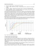
Fig. 13. System frequency deviation in case 4.
3.3 Frequency control in a hybrid wind-diesel power system using SMES
In this study, the system configuration in Fig. 5 is used to design frequency controller using
SMES. In worst case, it is assumed that the ability of the pitch controller in the wind side
and the governor in the diesel side to provide frequency control are is not adequate due to
theirs slow response. Accordingly, the SMES is installed in the system to fast compensate for
surplus or insufficient power demands, and minimize frequency deviation. Here, the
proposed method is applied to design the robust frequency controller of SMES.
3.3.1 Linearized model of hybrid wind-diesel power system with PPC and SMES
The linearized model of the hybrid wind-diesel power system with Programmed Pitch
Controller (PPC) and SMES is shown in Fig.14 (Tripathy, 1997). This model consists of the

following subsystems: wind dynamic model, diesel dynamic model, SMES unit, blade pitch
control of wind turbine and generator dynamic model. The details of all subsystems are
explained in (Tripathy, 1997). As shown in Fig. 15, the SMES block diagram consists of two
transfer functions, i.e. the SMES model and the frequency controller. Based on (Mitani et.al.
1988), the SMES can be modeled by the first-order transfer function with time constant
0.03
sm
T = s. In this work, the frequency controller is practically represented by a lead/lag
compensator with first order. In the controller, there are three control parameters i.e.,
sm
K ,
1sm
T and
2sm
T .
The linearized state equation of system in Fig. 14 can be expressed as

SM
XAXBu
•
Δ=Δ+Δ (11)

SM
YCXDu
Δ
=Δ+Δ (12)

SM SM IN
uKu
Δ

=Δ (13)
From Turbine to Wind Farms - Technical Requirements and Spin-Off Products

90

Fig. 14. Block diagram of a hybrid wind-diesel power generation with SMES.


Fig. 15. Block diagram of SMES with the frequency controller.
Where the state vector
[
]
T
MDFDW
PHHHPPffX ΔΔΔΔΔΔΔΔ=Δ
2101
, the output
vector
[]
D
fY Δ=Δ
,
D
f
Δ
is the system frequency deviation,
SMSES
P
Δ
is the control output

signal of SMES controller;
IN
u
Δ
=[
Y
Δ
] is the feedback input signal of SMES controller.
Note that the system in equation (11) is a single-input single-output (SISO) system. The
proposed method is applied to design SMES controller, and the system of equation (11) is
referred to as the nominal plant G
3.3.2 Optimization problem formulation
The optimization problem can be formulated as follows,
Minimize

(
)
1GGK
∞
− (14)
Subject to ,
s
p
ec s
p
ec
ζ
ζσσ
≥≤ (15)
Control Scheme of Hybrid Wind-Diesel Power Generation System

91
min max
KKK
≤
≤
min max
TTT≤≤
where
ζ
and
s
p
ec
ζ
are the actual and desired damping ratio of the dominant mode,
respectively;
σ
and
s
p
ec
σ
are the actual and desired real part, respectively;
max
K and
min
K
are the maximum and minimum controller gains, respectively;
max

T and
min
T are the
maximum and minimum time constants, respectively. This optimization problem is solved
by GA to search optimal or near optimal set of the controller parameters.
3.3.3 Designed results
In the optimization, the ranges of search parameters and GA parameters are set as follows:
s
pec
ζ
is desired damping ratio is set as 0.4,
s
pec
σ
is desired real part of the dominant mode is
set as -0.2, and
min
K are
max
K minimum and maximum gains of SMES are set as 1 and 60,
min
T and
max
T are minimum and maximum time constants of SMES are set as 0.01 and 5.
The optimization problem is solved by genetic algorithm. As a result, the proposed
controller which is referred as “RSMES” is given.
Table 2 shows the eigenvalue and damping ratio for normal operating condition. Clearly,
the desired damping ratio and the desired real part are achieved by RSMES. Moreover, the
damping ratio of RSMES is improved as designed in comparison with No SMES case.

Cases Eigenvalues (damping ratio)
NO SMES
-39.0043
-24.4027
-3.5072
-1.2547
-0.1851 ± j 0.671, ξ = 0.266
-0.5591 ± j 0.541, ξ = 0.719
RSMES
-39.5266
-24.4006
-2.1681
-1.3325
-17.782 ± j 5.339, ξ =0.958
-0.3050 ± j 0.539, ξ =0.492
-0.2012 ± j 0.268, ξ =0.600
Table 2. Eigenvalues and Damping ratio
To evaluate performance of the proposed SMES, simulation studies are carried out under
four operating conditions as shown in Table 1. In simulation studies, the limiter 0.01
−
pukW
0.01
SMES
P≤Δ ≤
pukW on a system base 350 kVA is added to the output of SMES
with each controller to determine capacity of SMES. The performance and robustness of the
proposed controllers are compared with the conventional SMES controllers (CSMES)
obtained from (Tripathy,1997). Simulation results under 4 case studies are carried out as
follows.
From Turbine to Wind Farms - Technical Requirements and Spin-Off Products

92
Case 1: Step input of wind power or load change
In case 1, a 0.01 pukW step increase in the wind power input are applied to the system at t =
0.0 s. Fig. 16 shows the frequency deviation of the diesel generation side which represents
the system frequency deviation. Without SMES, the peak frequency deviation is very large.
The frequency deviation takes about 25 s to reach steady-state. This indicates that the pitch
controller in the wind side and the governor in the diesel side do not work well. On the
other hand, the peak frequency deviation is reduced significantly and returns to zero within
shorter period in case of CSMES and the RSMES. Nevertheless, the overshoot and setting
time of frequency oscillations in cases of RSMES is lower than that of CSMES.
0 5 10 15 20 25 30
-3
-2
-1
0
1
2
3
x 10
-4
Time (sec)
System frequency deviation (pu Hz)


Without SMES
CSMES
RSMES

Fig. 16. System frequency deviation against a step change of wind power.

Next, a 0.01 pukW step increase in the load power is applied to the system at t = 0.0 s. As
depicted in Fig. 17, both CSMES and RSMES are able to damp the frequency deviation
quickly in comparison to without SMES case. These results show that both CSMES and
RSMES have almost the same frequency control effects.
Case 2: Random wind power input.
In this case, the system is subjected to the random wind power input as shown in Fig.18. The
system frequency deviations under normal system parameters are shown in Fig.19. Normal
system parameter is the design point of both CSMES and RSMES. By the RSMES, the
frequency deviation is significantly reduced in comparison to that of CSMES.
Next, the robustness of frequency controller is evaluated by an integral square error (ISE)
under variations of system parameters. For 100 seconds of simulation study under the same
random wind power in Fig.18, the ISE of the system frequency deviation is defined as
ISE of
100
2
0
DD
ff
dtΔ= Δ
∫
(16)
Control Scheme of Hybrid Wind-Diesel Power Generation System

93


0 5 10 15 20 25 30
-3.5
-3
-2.5

-2
-1.5
-1
-0.5
0
0.5
1
1.5
x 10
-4
Time (sec)
System frequency deviation (pu Hz)


Without SMES
CSMES
RSMES


Fig. 17. System frequency deviation against a step load change.


0 20 40 60 80 100
0
0.2
0.4
0.6
0.8
1
1.2

x 10
-3
Time (sec)
Random wind power deviation (pu kW)


Fig. 18. Random wind power input.
From Turbine to Wind Farms - Technical Requirements and Spin-Off Products

94
0 20 40 60 80 100
-1
-0.5
0
0.5
1
1.5
x 10
-5
Time (sec)
System frequency deviation (pu Hz)


CSMES
RSMES

Fig. 19. System frequency deviation under normal system parameters.
Fig.20 shows the values of ISE when the fluid coupling coefficient
f
c

K
is varied from -30 %
to +30 % of the normal values. The values of ISE in case of CSMES largely increase as
f
c
K

decreases. In contrast, the values of ISE in case of RSMES are lower and slightly change.



Fig. 20. Variation of ISE under a change of
f
c
K .
Case 3: Random load change.
Fig. 22 shows the system frequency deviation under normal system parameters when the
random load change as shown in Fig.21 is applied to the system. The control effect of
RSMES is better than that of the CSMES.
Control Scheme of Hybrid Wind-Diesel Power Generation System

95
0 20 40 60 80 100
0
0.2
0.4
0.6
0.8
1
1.2

1.4
x 10
-3
Time ( se c)
Random load power deviation (pu kW)

Fig. 21. Random load change.
0 20 40 60 80 100
-1.5
-1
-0.5
0
0.5
1
1.5
2
x 10
-5
Time (sec)
System frequency deviation (pu Hz)


CSMES
RSMES

Fig. 22. System frequency deviation under normal system parameters.
Case 4: Simultaneous random wind power and load change.
In case 4, the random wind power input in Fig. 18 and the load change in Fig.21 are applied
to the system simultaneously. When the inertia constant of both sides are reduced by 30 %
from the normal values, the CSMES is sensitive to this parameter change. It is still not able

to work well as depicted in Fig.23. In contrast, RSMES is capable of damping the frequency
oscillation. The values of ISE of system frequency under the variation of
f
c
K from -30 % to
+30 % of the normal values are shown in Fig.24. As
f
c
K
decreases, the values of ISE in case
of CSMES highly increase. On the other hand, the values of ISE in case of RSMES are much
lower and almost constant. These simulation results confirm the high robustness of RSMES
against the random wind power, load change, and system parameter variations.
From Turbine to Wind Farms - Technical Requirements and Spin-Off Products

96
0 20 40 60 80 100
-3
-2
-1
0
1
2
3
x 10
-5
Time (sec)
System frequency deviation (pu Hz)

CSMES
RSMES

Fig. 23. System frequency deviation under a 30 % decrease in
f
c
K


Fig. 24. Variation of ISE under a change in
f
c
K .
Finally, SMES capacities required for frequency control are evaluated based on
simultaneous random wind power input and load change in case study 4 in addition to a 30
% decrease in
f
c
K parameters. The kW capacity is determined by the output limiter -0.01 ≤
Δ
P
SMES
≤ 0.01 pukW on a system base of 350 kW. The simulation results of SMES output
power in case study 4 are shown in Figs. 25. Both power output of CSMES and RSMES are
in the allowable limits. However, the performance and robustness of frequency oscillations
in cases of RSMES is much better than those of CSMES.
Control Scheme of Hybrid Wind-Diesel Power Generation System

97
0 20 40 60 80 100

-1
-0.5
0
0.5
1
1.5
x 10
-3
Time (sec)
SMES output power (pu)


CSMES
RSMES

Fig. 25. SMES output power under a 30 % decrease in
f
c
K
5. Conclusion
Control scheme of hybrid wind-diesel power generation has been proposed in this work.
This work focus on frequency control using robust controllers such as Pitch controller and
SMES. The robust controllers were designed based on inverse additive perturbation in an
isolated hybrid wind – diesel power system. The performance and stability conditions of
inverse additive perturbation technique have been applied as the objective function in the
optimization problem. The GA has been used to tune the control parameters of controllers.
The designed controllers are based on the conventional 1
st
-order lead-lag compensator.
Accordingly, it is easy to implement in real systems. The damping effects and robustness of

the proposed controllers have been evaluated in the isolated hybrid wind – diesel power
system. Simulation results confirm that the robustness of the proposed controllers are much
superior to that of the conventional controllers against various uncertainties.
6. References
Ackermann, T. (2005), Wind Power in Power Systems, John Wiley & Sons.
Hunter R.E.G. (1994), Wind-diesel systems a guide to technology and its implementation,
Cambridge University Press.
Lipman NH. (1989), Wind-diesel and autonomous energy systems,
Elservier Science
Publishers Ltd
.
Bhatti T.S., Al-Ademi A.A.F. & Bansal N.K. (1997), Load frequency control of isolated wind
diesel hybrid power systems,
International Journal of Energy Conversion and
Management
, Vol. 39, pp. 829-837.
From Turbine to Wind Farms - Technical Requirements and Spin-Off Products

98
Das, D., Aditya, S.K., & Kothari, D.P. (1999), Dynamics of diesel and wind turbine
generators on an isolated power system,
International Journal of Elect Power & Energy
Syst.
, vol. 21, pp.183-189.
Mohan Mathur R & Rajiv K. Varma. (2002), Thyristor-based FACTS controllers for electrical
transmission Systems,
John Wiley.
Ribeiro P.F. , Johnson B.K., Crow M.L., Arsoy A. & Liu Y. (2001), Energy Storage Systems for
Advanced Power Applications,
Proc. of the IEEE, Vol. 89, No. 12, pp. 1744 –1756.

Schainker R.B. (2004), Executive Overview: Energy Storage Options for a Sustainable Energy
Future,
IEEE Power Engineering Society General Meeting, pp. 2309 – 2314.
Jiang X. & Chu X. (2001), SMES System for Study on Utility and Customer Power
Applications,
IEEE Trans. on Applied Superconductivity, Vol. 11, pp. 1765–1768.
Simo J.B. & Kamwa I. (1995), Exploratory Assessment of the Dynamic Behavior of Multi-
machine System Stabilized by a SMES Unit,
IEEE Trans. on Power Systems, Vol.10,
No.3, pp. 1566–1571.
Wu C.J. &. Lee Y.S. (1993), Application of Simultaneous Active and Reactive Power
Modulation of Superconducting Magnetic Energy Storage Unit to Damp Turbine-
Generator Subsynchronous Oscillations,
IEEE Trans. on Energy Conversion, Vol.8,
No.1, pp. 63–70.
Maschowski J. & Nelles D. (1992), Power System Transient Stability Enhancement by
Optimal Simultaneous Control of Active and Reactive Power,
IFAC symposium on
power system and power plant control
, Munich, pp. 271–276.
Buckles W. & Hassenzahl W.V. (2000), Superconducting Magnetic Energy Storage,
IEEE
Power Engineering Review
, pp.16–20.
Juengst K.P. (1998), SMES Progress,
Proc. of 15th International Conference on Magnet
Technology, Science Press
, pp. 18–23.
Rabbani M.G., Devotta J.B.X. & Elangovan . (1998), An Adaptive Fuzzy Controlled
Superconducting Magnetic Energy Storage Unit for Power Systems,

Energy
Conversion and Management
, Vol. 39, pp.931-942.
Devotta J.B.X. & Rabbani M.G. (2000), Application of Superconducting Magnetic Energy
Storage Unit in Multi-machine Power Systems,
Energy Conversion and Management,
Vol. 41, pp. 493-504.
Tripathy S.C. (1997), Dynamic Simulation of Hybrid Wind-diesel Power Generation System
with Superconducting Magnetic Energy Storage,
Energy Conversion and
Management
, Vol.38 , pp.919-930.
Ngamroo . (2005), An Optimization Technique of Robust Load Frequency Stabilizers for
Superconducting Magnetic Energy Storage,
Energy Conversion and Management,
Vol.46, pp.3060-3090.
Chu X., Jiang X., Lai Y., Wu X. & Liu W. (2001), SMES Control Algorithms for Improving
Customer Power Quality,
IEEE Trans. on Applied Superconductivity, Vol. 11, pp.1769-
1772.
Devotta J.B.X., Rabbani M.G. & Elangovan S. (1999), Application of Superconducting
Magnetic Energy Storage Unit for Damping of Subsynchronous Oscillations in
Power Systems,
Energy Conversion and Management, Vol.40, pp.23-37.
Abdelsalam M.K., Boom R.W & Perterson H.A. (1987) , Operation Aspects of
Superconducting Magnetic Energy Storage (SMES),
IEEE Trans. on Magnetics,
Vol.23, pp. 3275-3277.
Control Scheme of Hybrid Wind-Diesel Power Generation System

99
Banerjee S., Chatterjee J.K & Tripathy S.C. (1990), Application of Magnetic Energy Storage
Unit as Load Frequency Stabilizer,
IEEE Trans. on Energy Conversions, Vol. 5, No. 1,
pp. 46–51.
Tripathy S.C. & Juengst K.P. (1997), Sampled Data Automatic Generation Control with
Superconducting Magnetic Energy Storage in Power Systems,
IEEE Trans. on
Energy Conversions
, Vol. 12, No. 2, pp. 187–191.
Tripathy S.C., Balasubramanian R. & Chandramohanan Nair P.S. (1997), Adaptive
Automatic Generation Control with Superconducting Magnetic Energy Storage in
Power Systems,
IEEE Trans. on Energy Conversion, Vol. 7, No. 3, pp. 434–441.
Demiroren A., Zeynelgil H.L & Sengor N.S. (2003), Automatic Generation Control for Power
System with SMES by using Neural Network Controller,
Electrical Power
Components Systems
, Vol. 31, No.1, pp. 1–25.
Demiroren A. & Yesil E. (2004), Automatic Generation Control with Fuzzy Logic Controllers
in the Power System Including SMES Units,
Electrical Power Energy Systems, Vol. 26,
pp. 291–305.
Djukanovic M., Khammash M. & Vittal V. (1999), Sequential Synthesis of Structured
Singular Values Based Decentralized Controllers in Power Systems,
IEEE Trans. on
Power Systems
, Vol. 14, No. 2, pp. 635–641.
Yu X., Khammash M. & Vittal V. (2001), Robust Design of a Damping Controller for Static
Var Compensators in Power Systems,

IEEE Trans. on Power Systems, Vol. 16, No.3,
pp.456–462.
Zhu C., Khammash M. , Vittal V. & Qui W. (2003) , Robust Power System Stabilizer Design
using
H
∞
Loop Shaping Approach, IEEE Trans. on Power Systems, Vol. 18, No.2, pp.
810–818.
Rahim A.H.M.A. & Kandlawala M.F. (2004), Robust STATCOM Voltage Controller Design
using Loop-shaping Technique,
Trans. on Electric Power Systems Research, Vol. 68
No.1, pp. 61–74.
Wang Y., Tan Y.L. & Guo G. (2002), Robust Nonlinear Coordinated Excitation and TCSC
Control for Power Systems,
IEE Proc. of Generation Transmission and Distribution,
Vol. 149, No. 3, pp. 367–372.
Tan Y.L. & Wang Y. (2004), A Robust Nonlinear Excitation and SMES Controller for
Transient Stabilization,
Electrical Power Energy Systems, Vol. 26, No.5, pp. 325–332.
Gu P., Petkov Hr. & Konstantinov M.M.(2005), Robust Control Design with MATLAB,
Springer.
Abdel-Magid Y. L., Abido M. A., AI-Baiyat S. & Mantawy A. H. (1999), Simultaneous
Stabilization of Multimachine Power Systems via Genetic Algorithm,
IEEE Trans. on
Power Systems
, Vol. 14, No. 4, pp. 1428-1439.
GAOT (2005), A Genetic Algorithm for Function Optimization: A Matlab Implementation.
[Online] Available:
Goldberg D.E. (1989), Genetic Algorithm in Search, Optimization and Machine Learning,
Addison-Wesley Publishing Company Inc.

Das D., Aditya, S.K., & Kothari, D.P. (1999), Dynamics of diesel and wind turbine generators
on an isolated power system,
International Journal of Elect Power & Energy Syst., vol.
21, pp.183-189.
From Turbine to Wind Farms - Technical Requirements and Spin-Off Products

100
Tripathy SC . (1997), Dynamic simulation of hybrid wind-diesel power generation system
with superconducting magnetic energy storage,
Energy Conv and Manag. Vol. 38,
No. 9, 919-930.
Tripathy SC, Kalantar M & Balasubramanian R. (1991), Dynamic and stability of wind and
diesel turbine generators with superconducting magnetic energy storage unit on an
isolated power system,
IEEE Trans on Energy Conv , Vol. 6, No. 4, pp. 579-585.
Mitani Y, Tsuji K & Murakami Y. (1988), Application of superconducting magnetic energy
storage to improve power system dynamic performance ,
IEEE Trans. Power Syst ,
Vol. 3, No. 4, pp. 1418-25.
Panda S, Yadav J.S, Patidar N.P and Ardil C. (2009), Evolutionary Techniques for Model
Order Reduction of Large Scale Linear Systems,
International Journal of Engineering
and Applied Sciences
, Vol. 5, No.1, pp. 22-28.
Andrew C, Peter F, Hartmut P and Carlos F. Genetic Algorithm TOOLBOX For Use with
MATLAB- User’s guide, Department of automatic control and systems engineering,
university of Sheffield.
6
Power Fluctuations in a Wind Farm
Compared to a Single Turbine

Joaquin Mur-Amada and Jesús Sallán-Arasanz
Zaragoza University
Spain
1. Introduction
This chapter is focused on the estimation of wind farm power fluctuations from the
behaviour of a single turbine during continuous operation (special events such as turbine
tripping, grid transients, sudden voltages changes, etc. are not considered). The time scope
ranges from seconds to some minutes and the geographic scope is bounded to one or a few
nearby wind farms.
One of the objectives of this chapter is to explain quantitatively the wind power variability
in a farm from the behaviour of a single turbine. For short intervals and inside a wind farm,
the model is based on the experience with a logger system designed and installed in four
wind farms (Sanz et al., 2000a), the classic theory of Gaussian (normal) stochastic processes,
the wind coherence model (Schlez & Infield, 1998), and the general coherence function
derived by Risø Institute in Horns Rev wind farm (Martins et al., 2006; Sørensen et al.,
2008a). For larger distances and slower variations, the model has been tested with
meteorological data from the weather network.
The complexities inherent to stochastic processes are partially circumvented presenting
some case studies with meaningful graphs and using classical tools of signal processing and
time series analysis when possible. The sum of the power from many turbines is a stochastic
process that is the outcome of many interactions from different sources. The sum of the
power variations from more than four turbines converges approximately to a Gaussian
process despite of the process nature (deterministic, stochastic, broadband or narrowband),
analogously to the martingale central limit theorem (Hall & Heyde, 1980). The only required
condition is the negligible effect of synchronization forces among turbine oscillations.
The data logged at some wind farms are smooth and they have good mathematical
properties except during special events such as turbine breaker trips or severe weather. This
chapter will show that, under some circumstances, the power output of a wind farm can be
approximated to a Gaussian process and its auto spectrum density can be estimated from
the spectrum of a turbine, wind farm dimensions and wind coherence. The wind farm

power variability is fully characterized by its auto spectrum provided the Gaussian
approximation is accurate enough. Many interesting properties such as the mean power
fluctuation shape during a period, the distribution of power variation in a time period, the
more extreme power variation expected during a short period, etc. can be estimated
applying the outstanding properties of Gaussian processes according to (Bierbooms, 2008)
and (Mur-Amada, 2009).
From Turbine to Wind Farms - Technical Requirements and Spin-Off Products

102
Since the canonical representation of a Gaussian stochastic process is its frequency spectrum
(Karhunen–Loeve theorem), the analysis of wind power fluctuations is usually done in the
frequency domain for convenience. An alternative to Fourier analysis is time series analysis.
Time series are quite popular in stochastic models since they are well suited to prediction
and their parameters and their properties can be easily estimated (Wangdee & Billinton,
2006). Even though the two mathematical techniques are quite related, the study of periodic
behaviour is more direct through Fourier approach whereas the time series approach is
more appropriate for the study of non-systematic behaviour.
1.1 Sources of wind power fluctuation
The fluctuations observed at the output of a turbine are the outcome of the interaction of
wind turbulence with the complex turbine dynamics. For very slow fluctuations
(corresponding to lower frequencies in the spectrum), the turbine regulation achieves its
target and the turbine dynamics are negligible. Faster fluctuations (corresponding to higher
frequencies) interact with the structural and drive-train vibrations. The complexity of the
mechanical vibrations, the turbine control and the non-linearity of the generator power
electronics interactions affects notably the generator electromagnetic torque and the turbine
power fluctuations, especially in the frequency range from tenths of Hertzs to grid
frequency.
There are many dynamic turbine models described in the literature. Most megawatt
turbines share the following behaviour, considering the aerodynamic torque as the system
input and the power injected in the grid as the system output (Soens, 2005; Comech-Moreno,

2007; Bianchi et al, 2006):
• Between cut-in and rated wind speeds, the turbine power usually behaves (with
respect to the wind measured with an anemometer) as a low frequency first-order filter
with a time constant between 1 and 10 s.
• Between rated and cut-out wind speeds, the turbine power usually behaves (with
respect to the measured wind) as an asymmetric band pass filter of characteristic
frequency around 0,3 Hz due to the combined effect of the slow action of the
pitch/active stall and the quicker speed controllers.
• At some characteristic frequencies, the turbine mechanical vibrations, the power
electronics and the generator dynamics modify the general trend of the power output
spectrum with respect to the wind input.
There are many specific characteristics that impact notably the power fluctuations and their
realistic reproduction requires a comprehensive model of each turbine. The details of the
control, the structural details and the power electronics implemented in the turbines are
proprietary and they are not publicity available. In contrast, the electrical power injected by
a turbine can be measured easily.
Moreover, some fluctuations in power are not proportional to the fluctuations in wind or
aerodynamic torque. Thus, the ratio of the output signal divided by the input signal in the
frequency domain is not constant. However, a statistical linear model in the frequency can
be used (Welfonder et al., 1997) although the system output is neither proportional to the
input nor deterministic.
The approach taken in this chapter is primarily phenomenological: the power fluctuations
during the continuous operation of the turbines are measured and characterized for
timescales in the range of minutes to fractions of seconds. Thus, one contribution of this
Power Fluctuations in a Wind Farm Compared to a Single Turbine

103
chapter is the experimental characterization of the power fluctuations of three commercial
turbines. Some experimental measurements in the joint time-frequency domain are
presented to test the mathematical model of the fluctuations and the variability of PSD is

studied through spectrograms.
Other contribution of this chapter is the admittance of the wind farm: the oscillations from a
wind farm are compared to the fluctuations from a single turbine, representative of the
operation of the turbines in the farm. The partial cancellation of power fluctuations in a wind
farm is estimated from the ratio of the farm fluctuation relative to the fluctuation of one
representative turbine. Some stochastic models are derived in the frequency domain to link the
overall behaviour of a large number of wind turbines from the operation of a single turbine.
This chapter is based mostly on the experience obtained designing, programming,
assembling and analyzing two multipurpose measuring system installed in several wind
farms (Sanz et at., 2000a; Mur-Amada, 2009). This measuring system has been the first
prototype of a multipurpose data logger, now called AIRE (Analizador Integral de Recursos
Energéticos), that is currently commercialized by Inycom and CIRCE Foundation.
1.2 Random and almost cyclic fluctuations
Power output fluctuations can be divided into almost cyclic components (tower shadow,
wind shear, modal vibrations, etc.), wind farm weather dynamics (turbulence, boundary
layer atmospheric stability, micrometeorological dynamics, etc.) and events (connection or
disconnection of the turbine, change in generator configuration, etc.). The customary
treatment of these fluctuations is done through Fourier transform.
Cyclic fluctuations due to tower shadow, wind shear, etc. present more systematic
behaviour than weather related variations. Almost cyclic fluctuations are approximately
periodic and they present quite definite frequencies. In this context, almost periodic means
that the signal can be decomposed into a set of sinusoidal components with slow varying
amplitudes (some of them non-harmonically related) and stationary noise (i.e.,
polycyclostationary signals). The frequencies in the signal vary slightly since the fluctuation
amplitudes are not constant and the signal is not periodic in the conventional sense.


Fig. 1. Active power of a 750 kW wind turbine for wind speeds around 6,7 m/s during 20 s.
From Turbine to Wind Farms - Technical Requirements and Spin-Off Products

104
Cyclic variations are usually characterized with their Fourier transforms (Gardner, 1994).
Moreover, turbulence is also characterized through its auto spectral density, which is basically
the Fourier transform of its autocorrelation. Periodic fluctuations appear as narrow peaks at
their harmonic frequencies in the spectrum, whereas random fluctuations (which have neither
a periodic pattern nor a characteristic frequency) can be associated with the tendency of the
smoothed spectrum. Thus, the magnitude and frequency of the cyclic fluctuations can be
characterized for each turbine model and wind regime (Mur-Amada, 2009).
Weather evolution is the outcome of slow and complex atmospheric processes. Since
weather evolution has a strong non-linear behaviour, it will not be considered in this
chapter.
1.3 Fluctuations induced by the wind turbulence
Many fluctuations in the power output are strongly related to wind fluctuations, especially at
low frequencies (slow fluctuations). The wind spectrum is a common way to characterize the
frequency content of the turbulence present in the wind as it flows around an anemometer.
The wind is usually measured in a fixed point, but the wind varies along a wind farm, not only
due to the obstacles and orography, but also due to the turbulent nature of wind.
Taylor’s hypothesis of frozen turbulence is a simple model that relates spatial and temporal
variations of the wind. This hypothesis can be used to reconstruct the approximate spatial
structure of wind from measurements with an anemometer fixed at a point in space.
In fact, wind irregularities experienced by a turbine are also perceived by the next turbines
(usually with diverse magnitude and with some time delay). The area of influence of the
turbulence is related to the value of wind speed deviations (Cushman-Roisin, 2007). Higher
wind fluctuations usually imply larger spatial extent. Therefore, wind fluctuations are
usually experienced in close turbines with some time lag/lead Δt’ In Taylor’s Hypothesis of
“frozen turbulence”, the gust travel time in the wind direction Δt’ is the distance in
longitudinal direction divided by the wind speed (see Fig. 2). The wind measured at the
tower of Fig. 2 varies in 10 s due to a perturbation 100 m long travelling at the wind speed.

ΔU=+1 m/s
ΔU=–1 m/s
100 m
a) t
0
= 0
10 m/s
b) t
1
=
100 m
10 s
10 m/s
=

10 m/s
u
U
longitudinal

ΔU=+1 m/s
ΔU=–1 m/s

Fig. 2. Example of a idealized eddy of 100 m (represented by a cloud) passing through a
meteorological mast according to Taylor’s Hypothesis of “frozen turbulence”.
If the fluctuation arrives to another turbine inside the time interval [–Δt , +Δt ], then the phase
uncertainty in the frequency domain is [–2π f Δt , +2π f Δt] radians, where f is the considered
frequency. When f > 0,5/Δt, the phase is undetermined because the uncertainty of the phase
excess [–π, +π] (i.e. a cycle). At frequencies a few times higher than 0,5/Δt, the fluctuation of
Power Fluctuations in a Wind Farm Compared to a Single Turbine

105
frequency f is experienced by other turbines with a random phase difference almost uniformly
distributed and with comparable amplitude. In other words, the phase of the fluctuations in
the frequency domain are uncorrelated stochastically at f > 0,5/Δt although the amplitude
could show a systematic behaviour. The spatial and temporal coherence statistically quantifies
the variations of wind in different points in space or in separate moments of time.
For convenience, the wind is sometimes assumed barely uniform in the area swept by the
turbine. Based on this approximation, the equivalent wind is defined as the one that produces
the same effects that the non-uniform real wind field. Although the wind field cannot be
directly measured, its effects can be deduced from an equivalent wind that is usually
derived from the measurements of an anemometer, because variations in time and space are
related by the air flow dynamics.
The equivalent wind speed contains a stochastic component due to the effects of turbulence,
a rotational component due to the wind shear and the tower shadow and the average value
of the wind in the swept area, considered constant in short intervals. The rotational effects
(wind shear and tower effect) are barely related to wind turbulence. Since they interact with
the drive-train and control dynamics, they are modelled as an additional term in the
oscillations. The rotational/vibration/control dynamics are introduced in the equivalent
wind as a mathematical artifice to reproduce the power oscillations observed in the turbine
output. This simplification works relatively well since the vibration turbine dynamics
randomize the real dependence of the generator torque with the rotor angle.
The turbulence does not show characteristic frequencies and the wind spectrum is quite
smooth from very low frequencies up to tenths of Hertzs. In contrast,
rotational/vibration/control oscillations in the power output exhibit a more repetitive
pattern with determinate characteristic frequencies. Apart from their frequency distribution,
turbulence and other oscillations have similar stochastic properties and they can be
modelled with the same mathematical tools.
The combination of the small signal model and the wind coherence permits to derive the
spatial averaging of random wind variations. The stochastic behaviour of wind links the

overall behaviour of a large number of turbines with the behaviour of a single turbine.
It should be noted that the travel time of the turbulence between the turbines is the very
reason why fast fluctuations of turbine power generated by the turbulence are smoothed in
the wind farm output. That is also the reason why a Gaussian processes is well suited to
model the power fluctuations across a wind farm. Thus, the analysis carried out in this
chapter is in the frequency domain for convenience. Moreover, this behaviour also relates
the dimensions and geometry of the wind farm with the cut-off frequency of the smoothing
(the smoothing depends also on the wind coherence and direction).
The auto spectral density of the equivalent wind of a cluster of turbines can be obtained
from the wind spectra, the parameters of an isolated turbine, lateral and longitudinal
dimensions of the cluster region and the decay factor of the spatial coherence.
Fluctuations due to the real wind field along the swept area, vibrations and control effects
are added to the equivalent wind modifying its spectra. Thus, they can be aggregated in the
equivalent wind, provided a turbine transfer function among the power output and the
equivalent wind is stated. The turbine transfer function transforms the equivalent wind
oscillations into power oscillations. This simplification works relatively well since the
turbine vibration dynamics randomize the turbine output and the high frequency
turbulence at different turbines has a similar a stochastic behaviour than the
From Turbine to Wind Farms - Technical Requirements and Spin-Off Products

106
rotational/vibration/control oscillations: at high frequencies, fluctuations from turbulence,
vibration, generator dynamics and control are fairly independent between turbines,
statistically speaking.
The combination of the small signal model and the wind coherence permits to derive the
spatial averaging of random wind variations. Since fast turbulence and
rotation/vibration/control oscillations are almost stochastically independent among the
farm turbines, their outcome can be assessed analogously, although their respective sources
are very different physical phenomena.
Thus, the overall behaviour of a turbine cluster (with more than 8 turbines) can be derived

from the behaviour of a single turbine using a Gaussian model. The wind farm admittance is
the ratio of the fluctuations observed in the farm output respect the typical behaviour of one
of its turbines. The wind farm admittance can be estimated from experimental
measurements or from parameters of an isolated turbine, lateral and longitudinal
dimensions of the cluster region and the decay factor of the spatial coherence. Although the
model proposed is an oversimplification of the actual behaviour of a group of turbines
scattered across an area, this model quantifies the influence of the spatial distribution of the
turbines in the smoothing and in the frequency content of the aggregated power. This
stochastic model is in agreement with the experimental data presented at the end of this
chapter.
1.4 Interaction of wind with turbine dynamics
The interaction between wind fluctuations and the turbine is very complex and a thorough
model of the turbine, generator and control system is needed for simulating the influence of
wind turbulence in power output (Karaki et al., 2002; Vilar-Moreno, 2003). The control
scheme and its optimized parameters are proprietary and difficult to obtain from
manufacturers and complex to induce from measurements usually available.
The turbine and micro-meteorological dynamics transform the combination of periodic and
random wind variations into stochastic fluctuations in the power. These variations can be
divided into equivalent wind variations and almost periodic events such as vibration, blade
positions, etc. Turbulence, turbine wakes, gusts are highly random and do not show a
definite frequency (Sørensen et al., 2002; Sørensen et al., 2008). Non-cyclic power variations
are usually regarded as the outcome of the random component of the wind. They concern
the control (short term prediction) and the forecast (long horizon prediction). Artificial
Intelligence techniques and advanced filtering have been used for forecasting. Power
fluctuations of frequency around 8 Hz can eventually produce flicker in very weak networks
(Thiringer et al., 2004; Amaris & Usaola, 1997).
Both current and power can be measured directly, they can be statistically characterized and
they are directly related to power quality. Current is transformed and its level depends on
transformer ratio and actual network voltage. In contrast, power flows along transformers
and networks without being altered except for some efficiency losses in the elements. That is

why linearized power flows in the frequency domain are used in this chapter for
characterizing experimentally the electrical behaviour of wind turbines.
1.5 Major difficulties in the fluctuation characterization
A priori estimation of power fluctuations requires thorough models of the wind turbines
and turbulence. However, an empirical analysis is much simpler since distinct fluctuation
Power Fluctuations in a Wind Farm Compared to a Single Turbine

107
sources usually present characteristic frequencies or some trend in the spectrum. In the
following sections, a phenomenological and pragmatic approach will be applied to draw
some conclusions and to extrapolate results from empirical studies to general cases.
The tower shadow, wind shear, rotor asymmetry and unbalance, blade misalignments
produce a torque modulation dependent on turbine angle. This torque is filtered by turbine
dynamics and the influence in output power can be complex. The signals cannot be
considered truly periodic because neither the characteristic frequencies are constant (rotor
speed is not constant and hence, the frequency of fluctuations induced by rotational effects)
nor the frequencies are harmonically related. Some frequencies cannot be expressed as
multiple of the others because the tower, blades and cinematic train present characteristic
structural resonance frequencies different from the blade passing the tower frequency, f
blade
.
Moreover, turbine control, electric generator and power electronics introduce oscillations at
other frequencies.
The turbulence adds a “coloured noise” overimposed to the former oscillatory modes,
modulating cyclic vibrations and influencing rotor speed. The actual power is the outcome
of many processes that interact and the analysis in the frequency domain is a simplifying
approximation of a system driven by stochastic differential equations.
The first problem when analyzing power variations is that the contributions from rotor
sampling, vibration modes and turbulence-driven variations are aggregated.
The second difficulty is the fact that frequencies of almost cyclic contributions are neither

fixed nor are they multiple. Fourier coefficients are defined for periodic signals, but the sum
of periodic components not harmonically related is no longer periodic.
The third difficulty is that frequencies of contributions are overlapped. Fortunately,
characteristic frequencies (resonance and blade frequencies and its harmonics) have narrow
margins for given operational conditions, producing peaks in the spectrum where one
contribution usually predominates over the rest.
The forth difficulty is the turbulence, that introduces a non-periodic stochastic behaviour
interacting with periodic signals. Different mathematical tools are customarily used for
periodic and stochastic signals, increasing the difficulty of the analysis of these mixed-type
signals.
The cyclic fluctuations of the turbine power can be considered in the fraction-of-time
probability framework as the sum of sets of signals with different periods with additive
stationary coloured noise and, hence, almost cyclostationary (Gardner et al, 2006). Since
wind power is formed by the superposition of several almost cyclostationary signals whose
periods are not harmonically related, wind power is polycyclostationary.
2. Mathematical framework and notation
2.1 Model assumptions
According to (Cidrás et al., 2002), voltage drops can only induce synchronized power
fluctuations in a weak electrical network with a very steady and a very uniformly
distributed wind. Most grid codes have been modified to minimize the simultaneous loss of
generation during special events such as breaker tripping, grid transients, sudden voltages
changes, etc. Except during the previous events, the synchronization of power fluctuations
from a cluster of turbines is primarily due to wind variations that are slow enough to affect
several turbines inside a wind farm.
From Turbine to Wind Farms - Technical Requirements and Spin-Off Products

108
Experimental measurements have corroborated that blade synchronisation is unusual. In
addition, fluctuations due to turbine vibration, dynamics and control can be considered
statistically independent between turbines, whereas turbulence and weather dynamics are

partially correlated. Fortunately, slow fluctuations can be linked to equivalent wind
fluctuations through a quasi-static approximation based on the power curve of the turbines.
As an outcome, the total fluctuation from an area is best characterized as a stochastic signal
even though the fluctuations from single turbines have strong cyclic components. In other
words, the transformation of cyclic components into stochastic components eases the
treatment of wind farm power fluctuations.
For convenience, the signal duration will be considered short enough to be stationary
(atmospheric dynamics will be supposed not to change considerably during the sample).
Therefore, the average power (which corresponds to the zero frequency component of the
sample) will be considered a known parameter.
a) Stochastic spectral phasor density of the active power
If P(t) is the active power recorded in 0 ≤ t ≤ T, its conventional Fourier transform, denoted
by F, is scaled by a factor 1/√T to achieve an spectral measure whose main statistical
properties do not depend on the sample duration T.

{}
()
2
0
11
() () () ()
T
jf
jft
Pf Pf e Pte dt Pt
TT
ϕ
π−
≡≡ =
∫


F (1)
The factor 1/√T is between unity –used for pulses and signals of bounded energy– and 1/T
–used in the Fourier coefficients of pure periodic signals–.
Fortunately, definition (1) has the advantage that the variance of
()Pf

is the two-sided auto
spectral density,
2
|()|Pf

=
()
P
PSD f
, which is independent of sample length T and it
characterizes the process.
()Pf

will be referred as stochastic spectral phasor density of the
active power or just the (stochastic) phasor for short.
Historically, the term “power spectral density” was coined when the signal analyzed P(t)
was the electric or magnetic field of a wave or the voltage output of an antenna connected
to a resistor R. The power transferred to the load R at frequencies between
-/2
f
fΔ and
+/2
f

fΔ was 2· ()/
P
f
PSD f RΔ –that is proportional to
()
P
PSD f
and the frequency
interval. If P(t) is the electric or magnetic field of a wave, then the power density at
frequency f of that wave is also proportional to
·()
P
f
PSD fΔ
.
In this chapter, P(t) represents the power output of a turbine or a wind farm. The root mean
square value (RMS for short) of power fluctuations at frequencies between
-/2
f
fΔ and
+/2
f
fΔ is |()|·2·Pf fΔ

. Power variance inside the previous frequency range is
()·
P
PSD f fΔ . Hence,
()
P

PSD f
in this chapter does not represent a power spectral density
and this term can lead to misinterpretations. Therefore,
()
P
PSD f
will be referred in this
chapter as the auto spectral density although the acronym PSD (from Power Spectral
Density) is maintained because it is widespread. Sometimes
()
P
PSD f
will be replaced by
2
()
P
f
σ
to emphasize that it represents the variance spectral density of signal P at frequency f.
Fig. 3. shows the estimated PSD from 13 minute operation of a squirrel cage induction
generator (SCIG) directly coupled to the grid (a portion of the original data is plotted in Fig.
1). The original auto spectrum is plotted in grey whereas the estimated PSD is in thin black