Hydrodynamics Optimizing Methods and Tools Part 10 docx
Bạn đang xem bản rút gọn của tài liệu. Xem và tải ngay bản đầy đủ của tài liệu tại đây (2.4 MB, 30 trang )
Hydrodynamics – Optimizing Methods and Tools
258
presence of the submerged weir. Significant flow velocity change occurs over the top of the
weir. Because the water depth over the weir was small, comparable to the size of the ADVP
device, velocity measurement over the weir top was difficult. Similarly, the velocities at the
flow surface could not be measured. Due to these shortages one was unable to validate the
computed secondary flow direction at the surface. Confetti trace lines of the physical model
(Fig. 5d) and the particle trace lines released on the water surface level of the computed flow
field were compared. The distributions of these trace lines are very similar which indicate
the predicted surface velocity directions are consistent with the physical model.
Fig. 6 shows the surface elevation contour lines. A high pressure zone forms at upstream of
the weir with a low pressure zone forming just downstream. The well known pattern of
water surface superelevation in a bendway is altered significantly due to the presence of the
weir. Because the alignment is 20˚ toward upstream, the high pressure zone is located closer
to the outer bank and low pressure zone is closer to the tip of the weir and the inner bank.
The flow passing the top of the weir inevitably turns toward the inner bank under such a
pressure distribution. The pressure skew seems to be the key to understanding why the
secondary current near the weir changes direction and become favorable to navigation.
Fig. 6. Pattern of water surface elevation contour (m) near the submerged weir
Summarizing the observations in the physical model and numerical simulation, the flow
pattern sketch around a submerged weir is shown in Fig. 7. Upstream of the weir, the high
pressure zone slows down the approach flow and tends to force the flow to separate. The
general helical secondary flow pattern in the approach channel is thus being changed. The
high pressure difference across the weir (shown in Fig. 6) accelerates the flow which tends to
pass over the top of the weir perpendicularly and creates a recirculation zone behind the
weir near the bottom. This recirculation zone and the overtop flow are separated by a shear
layer. Due to the shape of the channel bed, the recirculation zone is approximately
triangular. In the deeper portion of the channel, the recirculation enhanced by the shear flow
is stronger and requires a longer distance to dissipate. This triangular recirculation zone can
be clearly seen in the physical experiments. After the flow has passed the weir, the flow
pattern caused by the weir dissipates gradually downstream. The distance to fully recover
the flow pattern depends on the flow condition and the weir configuration. This distance is
important for determining optimal weir spacing when a multiple weir design is considered.
Inner Bank
Outer Bank
Weir Tip
Weir shoulder
Submerged
Weir
0.24040
0.24028
0.24018
0.23994
0.23974
0.23944
0.23938
Flow
Contour lines of
water surface
elevation (m)
Turbulent Flow Around Submerged Bendway Weirs and Its Influence on Channel Navigation
259
Fig. 7. Flow structure around a submerged weir
3.4 Flow field of the helical secondary currents
In order to illustrate secondary flow patterns, the computed flow fields are presented in a
series of cross-sections. These cross-sections are aligned in the direction of the radius of
curvature; the secondary current was defined as the velocity normal to the main flow
direction. The main flow direction was defined as the mean flow direction in the channel
without the submerged weir. Additional simulations were conducted to compute the main
flow directions for each submerged weir case.
Fig. 8 shows the weir alignment near the bendway apex and the display cross-sections (J).
All the cross-sections are equally spaced (
l) along the centerline. For clarity, the spacing
between these sections in the figure was exaggerated. The secondary currents presented in
Fig. 9 are from some of these sections.
Fig. 8. Sketch of the simulation channel and the display cross-sections
Free surface
Submerged weir
Helical flow
Main flow
Helical flow
Recirculation zone
Δ
l=0.1968
m
Apex J=54
R=15.24
m
Flow
J
=5
7
J
=52
Weir
Hydrodynamics – Optimizing Methods and Tools
260
The cross-sections in Fig. 9 are from upstream (Fig. 9a) to downstream (Fig. 9k), with the
outer bank on the left and inner bank on the right side. The counter clockwise secondary
current shown in section 40 (Fig.9a), far upstream of the SW, is a typical helical flow pattern.
Closer to the SW in section 47 (Fig. 9b), the helical structure is altered because the main flow
decelerates and separates. Since the weir has an angle of 20
o
from the radius line, it
intercepts with several display sections (Fig. 8). The presence of the SW is reflected by
highly complex secondary current and strong vertical motion shown in section 49, 50, 51, 52,
(Fig. 9c, 9d, 9e, 9f) which cut across the SW.
Fig. 9. (a) (b) (c) (d). Secondary current in the approach flow
The single celled, counter-clockwise helical current in the approaching flow becomes three
cells behind the weir: the one in the center is strong and has inverse, clockwise direction;
the other two near the banks are weaker (Fig. 9g and 9h). The inverse cell appearing on
the right side of the weir is actually on the downstream side if one observes a top view of
the flow pattern. The inverse cell is strong near the weir and dissipates gradually
downstream, indicating that the influence of the weir is in a limited distance. The two
cells near the banks are much weaker than the inverse center cell, however, they are of the
same direction as that of the helical current in the approach flow. These two concomitant
circulations are partly driven by the inverse cell and partly influenced by the flow around
the tips of the weir. They gain strength gradually as the inverse cell is dissipated (Sec. 54,
58, 60, 66, Fig 9g, 9h, 9i, 9j). They finally reconnect and form a single helical current cell
Secon
d
a
r
yVec
t
o
r
1111 J= 40, 47, 49, 50
X
(
m
)
Z(m)
0.5 1 1.5 2 2.5 3
0.0
0.2
0.4
X
(
m
)
Z(m)
0.5 1 1.5 2 2.5 3
0.0
0.2
0.4
X
(
m
)
Z(m)
0.5 1 1.5 2 2.5 3
0.0
0.2
0.4
0.1 m/s
X
(
m
)
Z(m)
0.5 1 1.5 2 2.5 3
0.0
0.2
0.4
a
b
d
c
Turbulent Flow Around Submerged Bendway Weirs and Its Influence on Channel Navigation
261
across the channel (Sec. 78, Fig. 9k). The helical current will strengthen further downstream
until complete recovery.
Fig. 9. (e) (f) (g) (h) (i) (j) (k) Secondary flow passing the submerged weir
Secon
d
a
r
yVec
t
o
r
1111 J= 51, 52, 54, 58
X
(
m
)
Z(m)
0.5 1 1.5 2 2.5 3
0.0
0.2
0.4
0.1 m/s
X
(
m
)
Z(m)
0.5 1 1.5 2 2.5 3
0.0
0.2
0.4
X
(
m
)
Z(m)
0.5 1 1.5 2 2.5 3
0.0
0.2
0.4
X
(
m
)
Z(m)
0.5 1 1.5 2 2.5 3
0.0
0.2
0.4
Secon
d
a
r
yVec
t
o
r
1111 J= 60, 66, 78
X
(
m
)
Z(m)
0.5 1 1.5 2 2.5 3
0.0
0.2
0.4
0.1 m/s
X
(
m
)
Z(m)
0.5 1 1.5 2 2.5 3
0.0
0.2
0.4
X
(
m
)
Z(m)
0.5 1 1.5 2 2.5 3
0.0
0.2
0.4
e
f
g
h
i
j
k
Hydrodynamics – Optimizing Methods and Tools
262
Because of the inverse flow cell, the flow velocity near the centerline on the water surface is
toward the inner bank instead of the outer bank. This cell of secondary flow inverse to the
normal helical cell is beneficial to navigation because it cancels the effect of the general
helical current and realigns flow toward the inner bank. The foot print of the inverse
secondary current on the free surface is an area extending downstream from the SW. The
length, width, and location of this realigned area are important to the safety of channel
navigation. Since the flow velocity could not be measured close to water surface and the
measuring ranges were set near the SW, one could not directly validate the predicted
surface flow realignment. More detailed measurements covering the entire zone would be
necessary to confirm the numerical results.
4. Study of Victoria Bendway
4.1 River geomorphology, hydraulic structures and measured velocity data
In 1995, six submerged weirs were constructed on the outer bank of Victoria Bend in the
Mississippi River in an attempt to improve navigation conditions (Fig. 10). The effectiveness
of submerged weirs on surface flow realignment in Victoria Bendway (VBW) of the
Mississippi River was studied.
VBW is located at the confluence of the White River, between the State of Arkansas and
Mississippi. The discharge in the Mississippi River upstream of the VBW is influenced by
the White River. VBW is a highly curved bend, with a ratio of the radius of curvature to the
channel width varying from 1 to 3 approximately, depending on the river stage. It has a 108
o
heading change and a radius of 1280 m. It is expected that the secondary current would be
very strong in such a channel, which creates a navigation hazard to navigating barges.
The submerged weirs were oriented upstream with angle from 69 to 76 degrees between the
weirs and the bend longitudinal line. Post-construction surveys indicated deposition at the
upstream reach of the weir field and scouring throughout the rest of the weir system. Three
long spur dikes were constructed on the flood plain or point bar of the VBW. The effect of
these dikes is to converge the flow to the main channel, therefore the point bar is protected
from erosion, and the channel is re-aligned to enhance navigation.
A comprehensive survey of this reach was conducted by the US Army Corps of Engineers in
1998. The data were measured by acoustic devices with bed elevation referenced to a
Cartesian coordinate system. In addition to the bed elevations, velocity data were taken in
VBW using Acoustic Doppler Current Profiler instrumentation on June 11 and June 12, 1998.
Three velocity transects were taken adjacent to each of the six submerged weirs: one
upstream, one downstream, and one over the top of the weirs (Fig. 11). A few transects were
taken between weirs with others downstream of the weir field where strong scouring
occurred. Because of the highly turbulent flow in the bendway, the surveyed velocity
transects were not straight across the channel.
The flow discharge in these two days was about that of a one year return flow and almost
constant. The flow depth and width of the channel were large at this discharge with the flow
depth in the main channel at about 15-35 m. The depth clearance above the weirs for
navigation is about 6 m. The point bar was fully submerged with two of the three dikes
partially submerged and the third one (downstream) completely submerged at this flow
condition. The discharge was determined by integrating the measured flow flux in transects.
Integrations of the flow flux using the measured velocities in each survey path indicate these
surveys were quite consistent, resulting in a near constant discharge (~12,600 m
3
/s) with
only a few exceptions.
Turbulent Flow Around Submerged Bendway Weirs and Its Influence on Channel Navigation
263
Fig. 10. Victoria Bendway of the Mississippi River, the White River and submerged weirs
Fig. 11 shows the bathymetry of the VBW and the 34 survey transects for measuring the
velocity field. The weirs constructed in the main channel are depicted using contours of bed
elevation. At each survey point, three-dimensional velocities were obtained along a vertical
line at a number of points ranging from 5 to more than 100, depending on the flow depth.
The velocity data measured on June 11, have 17 sections with a total of 2210 survey points
while the data taken on June 12, include 17 transects with a total of 2494 survey points. Due
to turbulent flow and complex bed bathymetry, the transects could not be held straight,
particularly at where the point bar and thalweg meet. Actual transects are longer than those
shown in Fig. 11, extending from the outer bank onto the point bar. The survey paths shown
are the portion in the main channel consisting of about 35% of the total length of transects.
Because the beam angle of the ADCP was 20˚, the sampling diameter near the bottom of the
main channel (~30 meter deep) would be around 22 meters. This implies that scattering of
the data would be large, particularly close to the irregular part of the bed and weirs, and the
data may not be able to resolve flow structures in the weir field. Muste et al. (2004)
discussed factors influencing the accuracy of ADCP measurement in general and evaluated
a particular velocity profile measured in the middle of a straight reach of the Upper
Mississippi River (Pool 8 near Brownsville, MN). For a steady flow of 4.5 m deep at the
measuring point, sampling duration of 11 minutes were necessary at a fixed point to obtain
a stable mean velocity profile. The measured mean velocity could differ as much as 45% if
the sampling duration was less than 7 minutes. Since the flow velocity in the VBW was
stronger and the flow depth larger, the measured mean velocity therefore could have a
larger error because the survey vessel was moving continuously and the data was obtained
Arkansas
Mississippi
Mississippi
River
Dikes &
point bar
Old
White
River
White
River
3D Domain
Submerged
weirs
Hydrodynamics – Optimizing Methods and Tools
264
by averaging signals sampled in a short distance. The average time for measuring one
transect of the VBW was about 10 minutes and that for a point was a few seconds. The
velocities measured at the surface level often have large differences from those measured at
lower levels, due to perhaps the influence from navigation traffic in the river, the survey
vessel, or limitations of the measuring instrumentation.
Fig. 11. Bed bathymetry, submerged weirs and the survey paths in the main channel. Section
numbers are marked along the outer bank.
There was a large elevation difference between the main channel bed and the point bar,
particularly near the downstream of the bendway. The weir field has caused additional
Y
7500 8000 8500 9000
1500 2000 2500 3000 3500 4000
28.108
25.271
22.434
19.596
16.759
13.921
11.084
8.247
5.409
2.572
Bed Elevation
[m]
1
(
0
4
)
2
(
0
3
)
3
(
0
2
)
4
(
0
1
)
5
(
1
0
)
6
(
0
9
)
7
(
0
8
)
8
(
0
7
)
9
(
0
6
)
1
0
(
1
5
)
1
1
(
1
4
)
1
2
(
1
3
)
1
3
(
1
2
)
1
4
(
1
1
)
1
5
(
2
0
)
1
6
(
1
9
)
1
7
(
1
8
)
J
u
n
e
1
1
,
9
8
01 04
02 03
03 02
04 01
05 10
06 09
07 08
08 07
09 06
10 15
11 14
12 13
13 12
14 11
15 20
16 19
17 18
19 16
20 25
21 24
22 23
23 22
24 21
25 30
26 29
27 28
29 26
30 36
31 35
32 34
33 33
34 32
Section Numbers
1
8
(
1
7
)
J
u
n
e
1
2
,
9
8
2
0
(
2
4
)
1
9
(
1
6
)
2
1
(
2
3
)
2
2
(
2
2
)
2
3
(
2
1
)
2
4
(
3
0
)
2
8
(
2
6
)
2
7
(
2
7
)
2
6
(
2
8
)
2
5
(
2
9
)
2
9
(
3
6
)
3
0
(
3
5
)
3
1
(
3
4
)
3
2
(
3
3
)
3
3
(
3
2
)
34 ( 31 )
S
u
r
v
e
y
e
d
o
n
7500 8000 8500 9000
2000 3000 4000
Plot Survey line
1
(
0
4
)
2
(
0
3
)
3
(
0
2
)
4
(
0
1
)
5
(
1
0
)
6
(
0
9
)
7
(
0
8
)
8
(
0
7
)
9
(
0
6
)
1
0
(
1
5
)
1
1
(
1
4
)
1
2
(
1
3
)
1
3
(
1
2
)
1
4
(
1
1
)
1
5
(
2
0
)
1
6
(
1
9
)
1
7
(
1
8
)
J
u
n
e
1
1
,
9
8
01 04
02 03
03 02
04 01
05 10
06 09
07 08
08 07
09 06
10 15
11 14
12 13
13 12
14 11
15 20
16 19
17 18
19 16
20 25
21 24
22 23
23 22
24 21
25 30
26 29
27 28
29 26
30 36
31 35
32 34
33 33
34 32
Section Numbers
1
8
(
1
7
)
J
u
n
e
1
2
,
9
8
2
0
(
2
4
)
1
9
(
1
6
)
2
1
(
2
3
)
2
2
(
2
2
)
2
3
(
2
1
)
2
4
(
3
0
)
2
8
(
2
6
)
2
7
(
2
7
)
2
6
(
2
8
)
2
5
(
2
9
)
2
9
(
3
6
)
3
0
(
3
5
)
3
1
(
3
4
)
3
2
(
3
3
)
3
3
(
3
2
)
34 ( 31 )
7500 8000 8500 9000
2000 3000 4000
Plot Survey line
Measured sections
Spur dike
Submerged
weirs
Flow
Turbulent Flow Around Submerged Bendway Weirs and Its Influence on Channel Navigation
265
deposition and erosion at the upstream and downstream channel of the bendway,
respectively. The bed between the weirs was also severely scoured. The resistance of the
weir field would slow down the approach flow, stimulate deposition and cause additional
flow toward point bar. The scouring in and downstream the weir field may result from
additional turbulence due to the weirs and the reduced sediment load in the flow.
The approach of this study is to apply the 3D numerical model validated using experiment
data to simulate the flow and evaluate the effectiveness of weirs. The numerical solutions
provide a much higher resolution of the flow field and make it possible to resolve more
detailed flow around the submerged weirs. The field velocity measurements were used to
validate again the three-dimensional flow model. Comparison of the simulations for the pre-
and post-weir channel revealed the effect of the weirs on the flow pattern.
4.2 Numerical simulation and model validation
Although the three-dimensional velocity data obtained were very detailed, the resolution of
the three survey transects adjacent to a weir were not sufficient for analyzing the near field
flow and its effect on navigation. Because the river channel near the Victoria Bendway was at
the confluence with the White River, the channel pattern was complicated (Fig. 10). In order to
use available computational resources efficiently, the 3D simulation was limited to a short
bendway reach with a curved computational domain of 4.6 km along the main channel and 1.8
km wide in the apex section. A two-dimensional model (CCHE2D, Jia & Wang 1999; Jia et al.,
2002a) was used to simulate a much longer reach (a 33.866 km stretch) to calibrate the
resistance parameter and to establish initial flow, upstream and downstream boundary
conditions for the 3D simulation. The effective roughness heights of the channel were obtained
by calibration using measured water surface elevation along the channel. This roughness was
used for the 3D simulation with the exception of the surface roughness of the SW. It was
approximated to be one half of the gravel of which it was constructed. The upstream flow
boundary conditions for the 3D model (flow rate and direction distributions) were specified
with the 2D model results. The depth-averaged velocity at each point of the boundary of the
3D domain was converted to a logarithmic profile and no secondary flow was imposed since
the inlet boundary was located in a relatively straight portion of the channel (Fig. 10).
The extended 2D channel stretches upstream and downstream of the VBW with a mesh size
of 123 (transversal) x 622 (longitudinal); more than 50% of the horizontal mesh nodes were
in the range of the bendway where 3D computations were carried out. The 3D computation
is for the flow in the bend with a mesh of 123 (transversal) x 322 (longitudinal) x 11
(vertical); more vertical mesh points were located near the bed. Three 3D grids (G
1
:58x189x8,
G
2
:123x322x11, and G
3
:123x324x14) were tested. Using the three meshes, the RMS error of
the simulation results and the measured data were computed and indicated in Table 2. Non-
dimensional
u
and
v
are for the u and v velocity component, respectively. Computational
points in the domain are much more than those measured. RMS errors were computed
using measured data and computational results interpolated to the measuring point. The
error of simulations is considerably less in the upper part of the flow (less than 8 m from the
surface) than that in the lower part (deeper than 8 m from surface). The accuracy of the
simulations did not significantly improve when mesh resolution was increased. As was
mentioned earlier the scatter of the ADCP data was quite large particularly near the bed.
This is attributed to larger data scatter near the bed such that the numerical accuracy
improvement due to mesh refinement was much smaller than the data scattering.
Hydrodynamics – Optimizing Methods and Tools
266
Mesh No. of vertical points Zone of calculation
umean
U/
vmean
U/
G
1
8
Upper profile 0.219 0.269
Lower profile 0.363 0.34
G
2
11
Upper profile 0.218 0.262
Lower profile 0.36 0.336
G
3
14
Upper profile 0.220 0.269
Lower profile 0.36 0.337
U
mea
n
~1.4 m/s is the mean velocity for the entire reach. Upper profile is the water surface to the 8 meters
deep point, Lower profile is from the point to the bed.
Table 2. RMS error of the data and simulation results using three meshes
The mesh size of G
2
in the main channel ranges from 12 to 30 m, approximately. A
submerged weir was resolved by 15 to 20 grid points. The submerged weirs are the largest
resistance elements in the main channel. The back side slope of the weirs observed from the
bed topography is less than 15˚. The largest weir in the bendway was about 230 m long and
10 m high. The first weir upstream was hardly visible due to significant deposition in front
of the weir.
2D simulation was used as a tool to calibrate roughness of the channel. The calibrated
Manning’s coefficient n=0.037 is reasonable considering large scale of bed forms, the
number of structures (dikes, submerged weirs) built in this channel reach. Water stage data
on June 11, 1998, from five gauge stations along the reach of 2D simulation, were used for
the calibration. The calibrated Manning’s coefficient was then transformed to equivalent
roughness height for the three-dimensional model by using Strickler’s function
d
n
A
1/6
(11)
where A is an empirical constant which may represent both grain and form resistance
(A=19 according to Chien and Wan, 1999), and d (~0.121 m) is the effective roughness
height which is consistent with a large data set for the Mississippi River (van Rijn, 1989).
Graf (1998) showed that A could vary from 20 to 45 in rivers with cobble or gravel bed.
The effective roughness is used in the wall function for specifying hydraulic rough
boundary condition:
u
z
uz
0
0
1
ln( )
for
s
uk
70
(12)
s
zk
0
0.03
where u
o
is the near bed flow velocity, u
*
is shear velocity,
(=0.41) is the Karman’s
Constant, z is the distance from a wall,
is the fluid viscosity and k
s
(~d) is the roughness
height. Although roughness height can be converted from the Darcy-Weisbach factor,
Chezy’s coefficient or Manning’s coefficient more rigorously (van Rijn, 1989), Eq. 11 was
used for its simplicity. Since d was a calibrated parameter, it lumps many factors related to
the resistance such as bed forms and grain roughness. The three point-bar dikes are large
Turbulent Flow Around Submerged Bendway Weirs and Its Influence on Channel Navigation
267
and resolved by the 2D model. The area of the submerged weir field was less than two
percent of the 2D simulation domain; the effective roughness height thus evaluated was
affected by the weir field only slightly. Measurement of bed form in the Mississippi River
(Leclair, 2004) revealed that the size of dunes ranges from 120 to 11 m with height ranges
from 3 to 1 m; dune length near a bendway is about 69 m. Considering the mesh size of the
main channel (12-30 m), the bedforms were not resolved by the model. Therefore, it is
reasonable to model their resistance using a lumped effective roughness height, and the
computational grid was considered being over the roughness elements (Wu et al., 2000). The
mixing length and k-
turbulence closure schemes were applied in this study. Results
indicate that the solutions from these two schemes had no significant differences in terms of
defining the main and helical flow. Bed roughness varies spatially in the channel and the
effective roughness used was a constant calibrated according to water surface profile.
Fig. 12. Simulated flow pattern (velocity m/s) near water surface in Victoria Bendway
Fig. 12 demonstrates the simulated flow field near the free surface of the channel. For clarity,
the resolution (velocity points) shown is only a few percent of the original. The first and
second dikes on the point bar were submerged only slightly. They were treated as un-
submerged in the simulation. A large area of recirculation was present between the first and
second long spur dikes, with the recirculation lengths limited by the dike spacing. The
recirculation behind the second dike was limited closely behind it and small in size, due to
channel curvature. One can also observe the flow pattern from the point bar returning to the
main channel near the end of the bendway.
Contour lines of surface velocity magnitude on the background of bed elevation shading are
shown in Fig. 13. The river stage was high with the point bar and the third dike on the right
bank submerged. One can see the flow velocity variation along the channel due to the
existence of the second dike and weir structures. Because the water depth was less over the
submerged weirs, the flow accelerates over the weirs.
Fig. 14 shows the computed water surface elevation contour overlaying the image of bed
elevation. More contour lines are concentrated near the weir and show a similar pattern: the
contour lines align parallel to the weirs and widen near the tips of the weirs. This distribution
~ 2.1 m/s
Hydrodynamics – Optimizing Methods and Tools
268
Fig. 13. Simulated distribution of velocity magnitude (m/s) near the water surface level
Fig. 14. Water surface elevation contours (m) in the main channel with submerged weirs
would accelerate the flow over the weir top normally and tends to turn the flow toward the
inside of the bend. The helical current due to channel curvature is toward the outer bank;
therefore, such a surface elevation pattern resulting from the submerged weirs reduces the
strength of the helical current. In Fig. 6, the simulated surface elevation contours for the
experiment case was also aligned parallel to the weir, similar to this field case; although due
11.24 16.87 22.49 30.00
Bed elevation (m)
Flow accelerate
s
over submerged
weirs
1
2
3
4
5
6
Flow
Spur dike N o. 2
2
.
0
8
1
2
.
0
8
1
1
.
7
0
2
1
.
3
2
4
0
.
9
4
6
0.757
1
.
8
9
2
2
.
0
8
1
0.757
1.892
2
.
0
8
1
1
.
5
1
3
1.135
1.892
1.892
2
.
2
7
0
2
.
2
7
0
1
.
5
1
3
~400 m
W
Submerged
weirs
1
2
3
4
5
6
Flow
Spur dike No. 2
39.79
39.79
39.74
4
0
.
0
4
39.93
39.65
39.69
3
9
.
9
9
39.79
3
9
.
8
1
3
9
.
8
4
39.88
3
9
.
9
3
39.96
39.98
3
9
.
9
9
~400
m
W
2
W
1
W
3
W
4
W
6
W
5
Turbulent Flow Around Submerged Bendway Weirs and Its Influence on Channel Navigation
269
to the difference in channel bathymetry, flow depth, and weir size relative to channel, etc.,
the patterns of the simulated water surface in these two cases are not exactly the same.
However, the paralleled contours produce pressure gradients perpendicular to the weirs
and thus help improving navigation.
To evaluate the quality of numerical simulations, model validation was performed by
comparing the simulation and the measured 3D velocity data. Because the computational
mesh points were different from those of the velocity survey, one has to interpolate the
numerical solution to the 3D survey points. Inverse distance interpolation was used to
compute the velocity from the eight vortices of a hexahedral mesh cell containing a
measuring point.
u(m/s)
Depth (m)
-4 -3 -2 -1 0 1 2 3
0
5
10
15
Section 2 P oint 15
v(m/s)
Depth (m)
-4 -3 -2 -1 0 1 2 3
0
5
10
15
Section 2 Point 15
w(m/s)
Depth (m)
-0.9 -0.6 -0.3 0 0.3
0
5
10
15
Section 2 Point 15
Total Velocity (m/s)
Depth (m)
0 1 2 3 4 5 6 7
0
5
10
15
Section 2 P oint 15
u(m/s)
Depth (m)
-4 -3 -2 -1 0 1 2 3
0
5
10
15
20
25
Section 6 Point 15
v(m/s)
Depth (m)
-4 -3 -2 -1 0 1 2 3
0
5
10
15
20
25
Section 6 Point 15
w(m/s)
Depth (m)
-0.9 -0.6 -0.3 0 0.3
0
5
10
15
20
25
Section 6 Point 15
Total Velocity (m/s)
Depth (m)
0 1 2 3 4 5 6 7
0
5
10
15
20
25
Section 6 Point 15
u(m/s)
Depth (m)
-4 -3 -2 -1 0 1 2 3
0
5
10
15
Section 9 Point 15
v(m/s)
Depth (m)
-4 -3 -2 -1 0 1 2 3
0
5
10
15
Section 9 Point 15
w(m/s)
Depth (m)
-0.9 -0.6 -0.3 0 0.3
0
5
10
15
Section 9 Point 15
Total Velocity (m/s)
Depth (m)
0 1 2 3 4 5 6 7
0
5
10
15
Section 9 Point 15
Hydrodynamics – Optimizing Methods and Tools
270
u(m/s)
Depth (m)
-4 -3 -2 -1 0 1 2 3
0
5
10
15
20
25
Section 12 Point 24
v(m/s)
Depth (m)
-4 -3 -2 -1 0 1 2 3
0
5
10
15
20
25
Section 12 Point 24
w(m/s)
Depth (m)
-0.9 -0.6 -0.3 0 0.3
0
5
10
15
20
25
Section 12 Point 24
Total Velocity (m/s)
Depth (m)
0 1 2 3 4 5 6 7
0
5
10
15
20
25
Section 12 Point 24
u(m/s)
Depth (m)
-4 -3 -2 -1 0 1 2 3
0
5
10
15
20
25
Section 1 6 Point 18
v(m/s)
Depth (m)
-4 -3 -2 -1 0 1 2 3
0
5
10
15
20
25
Section 16 Point 18
w(m/s)
Depth (m)
-0.9 -0.6 -0.3 0 0.3
0
5
10
15
20
25
Section 16 Point 18
Total Velocity (m/s)
Depth (m)
0 1 2 3 4 5 6 7
0
5
10
15
20
25
Section 1 6 Point 18
u(m/s)
Depth (m)
-4 -3 -2 -1 0 1 2 3
0
5
10
15
20
25
Section 20 Point 18
v(m/s)
Depth (m)
-4 -3 -2 -1 0 1 2 3
0
5
10
15
20
25
Section 20 Point 18
w(m/s)
Depth (m)
-0.9 -0.6 -0.3 0 0.3
0
5
10
15
20
25
Section 20 Point 18
Total Velocity (m/s)
Depth (m)
0 1 2 3 4 5 6 7
0
5
10
15
20
25
Section 20 Point 18
u(m/s)
Depth (m)
-4 -3 -2 -1 0 1 2 3
0
5
10
15
Section 22 Point 15
v(m/s)
Depth (m)
-4 -3 -2 -1 0 1 2 3
0
5
10
15
Section 22 Point 15
w(m/s)
Depth (m)
-0.9 -0.6 -0.3 0 0.3
0
5
10
15
Section 22 Point 15
Total Velocity (m/s)
Depth (m)
0 1 2 3 4 5 6 7
0
5
10
15
Section 22 Point 15
Turbulent Flow Around Submerged Bendway Weirs and Its Influence on Channel Navigation
271
Fig. 15. Comparisons of computed and measured velocity profiles, along the main channel,
Victoria Bendway
Because there were more than 4500 survey points, it is impossible and unnecessary to show
all the comparisons. Instead, only a limited number of points are presented. Several vertical
profiles are selected along the main channel (Fig. 11). Some points are located in scour holes
between weirs, and others are very close to the weirs. Fig. 15 shows comparisons of these
velocity profiles. Along each profile, computed and measured velocity components u, v, w
and total velocity are compared. The depth of the flow at these survey points ranges from
less than 20 m to about 35 m. Results indicate that the computed velocity profiles are smooth
curves in most areas of the channel, with the velocity magnitude increasing toward water
surface. Most of the comparisons show adequate agreement between data and simulation,
particularly in trend. The agreement is generally better for points away from the weirs. No
recirculation zone was found behind the weirs in the field data. In general, measured data
show scatter and variation along vertical lines and transects, and the scatters appear to be
random. For example, at measuring point 30 of Section 28, the measured velocities indicate
stronger variations along the vertical. Distributions like this are often located either near
abrupt bed change or close to a weir. At these locations, turbulence would be very strong
and the upper and lower portion of the flow may have different directions. Simulating a
mean turbulent flow, the numerical model resulted in a much smoother flow field than the
measured velocities taken in highly turbulent and unsteady natural conditions.
Fig. 16 shows the computed and measured velocity magnitude at ten selected transects.
Comparisons at three levels 0.05h, 0.4h and 0.8h (from the bed to water surface) are
u(m/s)
Depth (m)
-4 -3 -2 -1 0 1 2 3
0
5
10
15
20
25
Section 26 Point 18
v(m/s)
Depth (m)
-4 -3 -2 -1 0 1 2 3
0
5
10
15
20
25
Section 26 Point 18
w(m/s)
Depth (m)
-0.9 -0.6 -0.3 0 0.3
0
5
10
15
20
25
Section 26 Point 18
Total Velocity (m/s)
Depth (m)
0 1 2 3 4 5 6 7
0
5
10
15
20
25
Section 26 Point 18
u(m/s)
Depth (m)
-4 -3 -2 -1 0 1 2 3
0
5
10
15
20
25
Section 28 Point 30
v(m/s)
Depth (m)
-4 -3 -2 -1 0 1 2 3
0
5
10
15
20
25
Section 28 Point 30
Total Velocity (m/s)
Depth (m)
0 1 2 3 4 5 6 7
0
5
10
15
20
25
Section 28 Point 30
w(m/s)
Depth (m)
-0.9 -0.6 -0.3 0 0.3
0
5
10
15
20
25
Section 28 Point 30
Hydrodynamics – Optimizing Methods and Tools
272
presented. One finds general agreements along each level and section. The data scatter near
the channel bed is, in general, greater than in the upper portion of the water column,
consistent with the RMS errors indicated in Table 2, which could be resulted from the large
near-bed sampling volume of the ADCP and complex channel topography. The
comparisons were performed for the main channel rather than the point bar, because the
main interest of this study was the flow characteristics in the main channel. Although the
differences between the computed and measured data are large for many points, the trend
of the numerical results generally agrees with the data, particularly near the free surface
(0.8h). These comparisons (Fig. 15 and Fig. 16) have confirmed the consistency of the
numerical model with the field data and its applicability to this particular problem.
0 100 200 300 400
0
1
2
3
Section 3
U(m/s)
0 100 200 300 400
0
1
2
3
Section 27
U(m/s)
0 100 200 300 400
0
1
2
3
Section 23
U(m/s)
L(m)
0 100 200 300 400
0
1
2
3
Section 19
U(m/s)
0 100 200 300 400
0
1
2
3
Section 12
U(m/s)
L(m)
0 100 200 300 400
0
1
2
3
Section 34
U(m/s)
0 100 200 300 400
0
1
2
3
Section 1
U(m/s)
0 100 200 300 400
0
1
2
3
Section 9
U(m/s)
0 100 200 300 400
0
1
2
3
Section 25
U(m/s)
0 100 200 300 400
0
1
2
3
Field Data
CCHE3D
Section 21
U(m/s)
y/h = 0.80
(a)
Turbulent Flow Around Submerged Bendway Weirs and Its Influence on Channel Navigation
273
0 100 200 300 400
0
1
2
3
Section 3
U(m/s)
0 100 200 300 400
0
1
2
3
Section 27
U(m/s)
0 100 200 300 400
0
1
2
3
Section 23
U(m/s)
0 100 200 300 400
0
1
2
3
Section 12
U(m/s)
L(m)
0 100 200 300 400
0
1
2
3
Section 34
U(m/s)
0 100 200 300 400
0
1
2
3
Section 1
U(m/s)
0 100 200 300 400
0
1
2
3
Section 9
U(m/s)
0 100 200 300 400
0
1
2
3
Section 25
U(m/s)
L(m)
0 100 200 300 400
0
1
2
3
Section 19
U(m/s)
0 100 200 300 400
0
1
2
3
Field Data
CCHE3D
Section 21
U(m/s)
y/h = 0.60
(b)
Hydrodynamics – Optimizing Methods and Tools
274
0 100 200 300 400
0
1
2
3
Section 1
U(m/s)
0 100 200 300 400
0
1
2
3
Section 3
U(m/s)
0 100 200 300 400
0
1
2
3
Section 23
U(m/s)
0 100 200 300 400
0
1
2
3
Section 9
U(m/s)
0 100 200 300 400
0
1
2
3
Section 25
U(m/s)
0 100 200 300 400
0
1
2
3
Section 12
U(m/s)
0 100 200 300 400
0
1
2
3
Section 27
U(m/s)
L(m)
0 100 200 300 400
0
1
2
3
Section 19
U(m/s)
L(m)
0 100 200 300 400
0
1
2
3
Section 34
U(m/s)
0 100 200 300 400
0
1
2
3
Field Data
CCHE3D
Section 21
U(m/s)
y/h = 0.40
(c)
Turbulent Flow Around Submerged Bendway Weirs and Its Influence on Channel Navigation
275
Fig. 16. Comparison of computed and measured flow velocity at selected sections (a) near
water surface (z/h=0.8); (b) near middle depth (z/h=0.6); (c) near middle depth (z/h=0.4);
and (d) near bed (z/h=0.05).
0 100 200 300 400
0
1
2
3
Section 3
U(m/s)
0 100 200 300 400
0
1
2
3
Section 27
U(m/s)
L(m)
0 100 200 300 400
0
1
2
3
Section 19
U(m/s)
L(m)
0 100 200 300 400
0
1
2
3
Section 34
U(m/s)
0 100 200 300 400
0
1
2
3
Section 1
U(m/s)
0 100 200 300 400
0
1
2
3
Section 9
U(m/s)
0 100 200 300 400
0
1
2
3
Section 25
U(m/s)
0 100 200 300 400
0
1
2
3
Section 12
U(m/s)
0 100 200 300 400
0
1
2
3
Field Data
CCHE3D
Section 21
U(m/s)
y/h = 0.05
0 100 200 300 400
0
1
2
3
Section 23
U(m/s)
(d)
Hydrodynamics – Optimizing Methods and Tools
276
4.3 Helical secondary current and submerged weirs
Fig. 17 shows a plan view of the simulated 3D flow and comparison of computed and
measured secondary flows in a transect. Vectors (in red) at surface level (Fig. 17a) are
plotted with those near the bed (in black). The difference in their directions at each point
represents the helical current. For clarity, only a limited number of vectors are shown.
Looking upstream, the main helical current in the main channel is clockwise. The secondary
flow near the tip of the spur dike is also clockwise, but has been weakened or even reversed
at some locations. Since it does not follow the channel curvature, the flow over the point bar
goes directly into the main channel and alters the main flow there.
Fig. 17. Simulated secondary helical current in the bendway. a) General flow pattern; b)
Measured secondary velocity in the main channel near the point bar; and c) Computed
secondary velocity in the main channel near the point bar.
11.24 16.8 7 22 .49 30.00
Bed elevation (m)
Weir 1
Weir 2
Weir 3
Weir 4
Weir 5
Weir 6
Spur dike
No. 2
b. Measurement
c. Simulation
Section No. 30
Outer
bank
a. Simulated secondary
flow distribution
Turbulent Flow Around Submerged Bendway Weirs and Its Influence on Channel Navigation
277
The flow over the point bar starts to converge back to the main channel at the downstream
port of the bend. The returning flow near the edge of the point bar is not parallel to the edge;
the component normal to the main flow affects secondary current in the main channel. With
this particular bendway morphology configuration, the flow from the point bar back to the
main channel tends to enhance the helical current. Since the main channel deepens near the
6
th
SW, a large bed elevation step appears between the point bar and the main channel.
Affected by the flow from the point bar, the secondary current in the main channel appears
to be intensified (around survey section 30, Fig. 11), as indicated by measurement (Fig. 17b)
and simulation (Fig. 17c). The influence on the channel flow is similar to those observed by
Sellin (1995) and by Shiono & Muko (1998) in their experiments in which the flow from a
flood plain affects the secondary flow in the main channel. This indicates that the helical
flow in the main channel is strengthened, consistent with the observation that severe
channel erosion occurs on the downstream portion of the bend.
5. Influence of submerged weirs on navigation in VBW
Navigation problems in bendways are mainly attributed to the helical secondary current
which tends to push vessels toward the outer bank (the inertial and centrifugal forcing due
to the vessel’s own motion are not considered). The simulated secondary flows with and
without the submerged weirs were compared to assess the effectiveness of these weirs in
reducing the strength of the secondary flow. The submerged weirs were removed from the
computational domain; the deposition and erosion patterns, due to the presence of the
weirs, were corrected using the channel bathymetry (cross-sections) surveyed in 1994 before
the weir field installation as a reference. A 2D simulation was also conducted for producing
boundary conditions.
The influence of the submerged weirs on the helical current was evaluated by the difference
in the secondary current with and without weirs. Fig. 18a shows the computed secondary
current in sections upstream, over, and downstream submerged weir No. 4. The orientation
of these sections was approximately normal to the main flow direction. The secondary flow
is strongly changed by this submerged weir. In the section over the weir, the changes in the
secondary flows are dramatic. Near the water surface, the transversal flow toward the outer
bank is reduced or reversed. Because vessels in bendways are pushed laterally by the
transverse flow, this submerged weir effect would be beneficial to the channel navigation. In
sections between weirs, the secondary current tends to recover the normal pattern of curved
channel flows. Fig. 18b shows the computed helical current in the corresponding sections
without the submerged weir.
The direction of the near surface flow defined by the angle
transversal
lon
g
itudinal
u
u
arctan
(14)
was used as an indicator of the flow alignment or navigation condition in bendways. If the
angle (
) is very small, the navigation condition is considered good because the flow would be
aligned more along the main channel. To evaluate how the weir system influenced the flow
angle, the difference of the flow angle at the free surface in the main channel with and without
weirs,
=
with weirs
-
without weirs
) was computed and presented in Fig. 19. Considering the
secondary flow is normally in the order of 0.1u
longitudinal
, or less, the change of flow angle in the
order of 5.7 degree would be sufficient to cancel the near surface secondary velocity.
Hydrodynamics – Optimizing Methods and Tools
278
Fig. 18. Secondary currents around submerged weir No. 4; a) with weirs, b) without weirs
Fig. 19. The difference of the flow angles between the flows with and without submerged
weirs. Only the main channel is shown. The portion with improved condition (with negative
) is shaded.
x
y
7500 8000 8500
2000
2500
3000
3500
4000
-2.054
-4.468
-6.882
Angle (degree)
1
2
3
4
5
6
Outer bank
Flood Plain
(a)
Upstream sectio
n
Outer bank
Flood Plain
(b)
Upstream
Over weir section
Over weir section
Downstream sectio
n
Downstream sectio
n
Point bar
Location of
submerged
weirs
Turbulent Flow Around Submerged Bendway Weirs and Its Influence on Channel Navigation
279
The areas with a negative angle represent where the flow condition is improved, whereas
the areas with a positive value indicate where the condition became worse. To distinguish
the areas with an improved condition, the contours of the area with a worsened condition is
replaced with white. It is seen that the total improved area is larger than 50% and that
conditions are better near the weirs. The flow angle change is high over the weir tops and
low between them. The maximum angle change reaches about 6.8˚ with less change between
weirs. The flow condition near weir No. 6 is worsened, because the strong flow from the
point bar returns to the main channel and the secondary current intensifies. After the
construction of the weirs, the resistance of the main channel increased resulting in more
water flowing over the point bar at the entrance of the bend and then returning to the main
channel. The strength of the secondary current near weir No. 6 is thus increased (Fig. 17).
The excessive deposition upstream of the weir field in the main channel has disabled the
first weir; thus, the first weir is not functional (Fig. 19). In addition, the first and last weir
were angled less than others, so they should be less effective even without the influence of
the flow from the point bar and sedimentation. To a certain extent, a weir would be more
effective if it is angled more toward upstream; its effect on realigning the flow is also
influenced by relative length, relative depth, and channel curvature, etc. (Jia et al., 2002b).
Future submerged weir designs should consider the influence of local morphology (flood
plain). Since the influence of the weirs varies in terms of water depth and relative weir
height, additional studies with several more flow conditions are necessary to enhance
submerged weir designs.
6. Conclusions
A three-dimensional computational model for free surface turbulent flows, CCHE3D, has
been applied to study flows in bendways affected by submerged weirs. Both experimental
data and field data were used for model validation. The flow distribution due to a weir in a
bendway was discussed and the effect of multiple weirs in the Victoria Bendway in the
Mississippi River on channel navigation was studied. The comparisons showed good
agreement in both the experiment and field cases between measured and simulated data
which confirmed the consistency of the numerical model, the physical model and the large
scale field case.
The general helical secondary current pattern in the experimental channel was disturbed by
the single weir, particularly in its vicinity. In the experiments with a submerged single weir,
it was found that the weir resulted in a high pressure zone forming on its upstream side and
a low pressure zone on the downstream side. The high pressure zone slows the approaching
flow and tends to separate it, forcing more flow toward the ends of the weir with the
velocities near the tips increasing and higher than in the center region of the weir and the
channel. The low pressure behind the weir creates a triangle-shaped recirculation zone. Due
to the alignment of the weir (angled toward upstream), the high pressure and the low
pressure zones are not located along the general stream direction. The high pressure zone is
located closer to the outer bank and the low pressure zone is closer to the inner bank (tip of
the weir). The skewed distribution tends to realign the overtopping flow toward the inner
bank, which is opposite to the general helical current direction. The realigned surface
current and the recirculation behind the weir form an inverse secondary cell. Two weaker
secondary cells along the banks were also observed parallel to the inverse cell.
Hydrodynamics – Optimizing Methods and Tools
280
Due to the submerged weir, the flow velocity near the center of the experimental channel
decreases and that near the tips of the weir increases. These high velocity zones may result
in bed erosion and channel widening. The contours of the water surface are parallel to the
weir direction and surface flow direction was realigned to the inner bank, thus being
favorable to navigation. The effect of the weir is limited, and normal curved channel flow
pattern may recover downstream. Further research is necessary to quantify sediment
transport characteristics of bendways containing submerged weir fields.
In Victoria Bendway with multiple weirs, the simulation indicated that the helical current
was only significant in the main channel. The flow over the point bar has little curvature and
secondary current structure under the flow conditions studied is very weak. The helical
current in the main channel was enhanced by the flow returning back to the main channel
from the point bar.
For the case of Victoria Bendway, the computed velocities were smooth curves varying in
the vertical direction, while the measured velocities show scatters much larger than the
experiment case. Because of the nature of the ADCP instrument, the scatters are particularly
strong near the bed, in close vicinity of weirs, and where the main channel and point bar
join. A larger discrepancy of velocity comparisons would appear in these areas. The
comparisons along measured transects at several vertical levels show reasonable agreement
with the best agreement appearing near the water surface (0.8h).
In the main channel of Victoria Bendway, the direction and magnitude of the secondary
current were affected by the submerged weirs. Not only was the secondary current structure
changed, the secondary flow near the free surface around the weirs was weakened. This is
consistent with the simulated water surface elevation pattern which tends to realign the
flow over the top of the weirs. The way the flow is affected by these weirs is similar to that
observed in the experimental channel of the physical model.
To study the overall effectiveness of the weir field, numerical simulations without weirs
were also carried out and the solutions were compared to that with weirs in Victoria
Bendway. Flow direction change in the main channel was compared and the weir
effectiveness was evaluated. Most of the weirs (four out of six) were found effective, but the
first and last weir were not. The ineffectiveness was caused by the channel deposition and
the flow returning from the point bar enhanced the helical current. In addition, a smaller
alignment angle made them less effective.
7. Acknowledgement
This investigation was conducted under contract agreement No. DACW42-01-P-0243 and
No. DACW42-00-P-0456 with the US Army Corps of Engineers, Waterways Experimental
Station, and the National Center for Computational Hydroscience and Engineering, The
University of Mississippi. Professor Pierre Julien of Colorado State University provided
valuable suggestions in reviewing a part of this study. Mr. Michael F. Winkler of USACE
provided the physical model data. The authors appreciate the help of Dr. Yaoxin Zhang at
NCCHE for his technical assistance.
8. References
Bhuiyan, A.B.M.F. & Hey, R.D. (2001). Instream J-vane for bank protection and river
restoration, XXIX IAHR Congress Proceedings, Beijing, China. Theme D, Vol. II, pp
161-166.
Turbulent Flow Around Submerged Bendway Weirs and Its Influence on Channel Navigation
281
Bhuiyan, F & Olsen, N.R.B., (2002). Three-dimensional numerical modeling of flow and
scour around spur-dikes, Proceedings of the Fifth International Conference on
Hydroinformatics, Cardiff, UK, 2002, 70-75
Blanckaert, K. & Graf, W.H. (2001). Mean flow and turbulence in open-channel bend, J.
Hydraulic Eng., 127(10), 835-847.
Booij, R. (2003). Modeling the flow in curved tidal channels and rivers, Proceedings,
International Conference on Estuaries and Coasts, Nov. 11, 2003, Hangzhou, China,
pp786-794.
Chien, N. & Wan, Z. (1999). Mechanics of Sediment Transport, ASCE press, ASCE, 1801
Alexander Bell Drive, Reston, Virginia 20191-4400.
Davinroy, R. D. & Redington, S.L. (1996). Bendway weirs on the Mississippi River, a
status report, Proceedings of the 6th Federal Interagency Sedimentation Conference,
March 10-14, 1996, Las Vegas, NV, pp III32-37.
De Vriend, D.J. (1979). Flow measurements in a Curved Rectangular Channel, Laboratory of
Fluid Mechanics, Department of Civil Engineering, Delft University of
Technology, Internal Report No. 9-79.
Duan J.G., Wang, S.S.Y., & Jia, Y. (2001). The application of the enhanced CCHE2D
model to study the alluvial channel migration processes, J. Hydraul. Res., 39(5)
2001, 469-480.
Graf, W.H. (1998). Fluvial Hydraulics, John Willey & Sons Ltd, Baffins Lane, Chichester,
West Sussex PO19 1UD, England.
Hsieh, T.Y. & Yang, J.C. (2003). Investigation of the suitability of two-dimensional depth-
averaged models for bend flow simulation, J. Hydraul. Eng., 129(8), 597-612.
Jarrahzade, F. & Bejestan, M.S. (2011). Comparison of maximum scour depth in Bank line
and nose of submerged weirs in a sharp bend, Scientific Research and Essays, Vol.
6(5), pp. 1071-1076, 4 March, 2011, available online at
Jia, Y., & Wang, S.S.Y. (1992). Computational model verification test case using flume
data, Proceedings: Hydraulic Eng., 436-441, ASCE.
Jia, Y., & Wang, S.S.Y. (1993). 3D Numerical Simulation of Flow Near a Spur Dike,
Advances in HydroScience and Engineering, Proceedings of International Conference for
Hydroscience and Engineering, Vol. I Part B, pp2150-2156. University of
Mississippi, June, 1993.
Jia, Y & Wang, S.S.Y. (1999). Numerical model for channel flow and morphological change
studies, J. Hydraul. Eng., ASCE, 125(9), 924-933.
Jia, Y., & Wang, S.S.Y. (2000a). Numerical Study of Turbulent Flow around Submerged
Spur Dikes, 2000 International Conference of Hydroscience and Engineering, Korea.
Jia, Y., & Wang, S.S.Y. (2000b). Numerical simulations of the channel flow with
submerged weirs in Victoria Bendway, Mississippi River, Technical Report No.
NCCHE-TR-2000-3, National Center for Computational Hydroscience and
Engineering, The University of Mississippi.
Jia, Y., Blanckaert, K., & Wang, S.S.Y. (2001a). Simulation of secondary flow in curved
channels, Proceedings of the FMTM2001 International Conference, Tokyo, Japan.