báo cáo hóa học: " A cost model for optimizing the take back phase of used product recovery" docx
Bạn đang xem bản rút gọn của tài liệu. Xem và tải ngay bản đầy đủ của tài liệu tại đây (1.35 MB, 15 trang )
RESEARCH Open Access
A cost model for optimizing the take back phase
of used product recovery
Niloufar Ghoreishi
1*
, Mark J Jakiela
1
and Ali Nekouzadeh
2
Abstract
Taking back the end-of-life products from customers can be made profitable by optimizing the combination of
advertising, financial benefits for the customer, and ease of delivery (product transport). In this paper we present a
detailed modeling framework developed for the cost benefit analysis of the take back process. This model includes
many aspects that have not been modeled before, including financial incentives in the form of discounts, as well
as transportation and advertisement costs. In this model customers are motivated to return their used products
with financial incentives in the forms of cash and discounts for the purchase of new products. Cost and revenue
allocation between take back and new product sale is discussed and modeled. The frequency, method and cost of
advertisement are also addressed. The convenience of transportation method and the transportation costs are
included in the model as well. The effects of the type and amount of financial incentives, frequ ency and method
of advertisement, and method of transportation on the product return rate and the net profit of take back were
formulated and studied. The application of the model for determining the optimum strategies (operational levels)
and predicting the maximum net profit of the take back pro cess was demonstrated through a practical, but
hypothetical, example.
Keywords: Take Back, Product Acquisition, Remanufacturing, Modeling, Cost Benefit Analysi s
Introduction
Taking back used products is the first step in mos t of
the end of life (E.O.L) recovery options which include
remanufacturing, refurbishment, reuse, and recycling.
“Take back” include s all the activi ties involved in trans-
ferring the used product from the customers’ possession
to the recovery site. In general optimizing of the take
back (also called product acquisition) has received lim-
ited attention in research and ope rations. Guide and
Van Wassenhove categorized take back processes into
two groups: waste stream and market dr iven [1]. In a
waste stream process, the collecting firm cannot control
the quality and quantity of the used products: all the E.
O.L. products will be collected and transferred. In a
market driven process, customers are motivated to
return the end o f life product by some type of financial
incentive.Thisway,the(re)manufacturer can control
the quantity and quality of the returned products
through the amount and type of incentives and increase
its profit [2-4].
In general the taking-back firm can control the pro-
cess by setting strategies regarding financial incentives,
advertisement, and collection/transportation methods
[2,3,5-8]. Usually, offering higher incentives (in the form
of cash or discounts toward purchasing n ew products)
will increase the return rate and lead to acquisition of
higher quality used products. Higher incentives s ome-
times can encourage the customers to replace their old
products with a new one earlier [9]. Another way to
control the quality of the used product is to have a sys-
tem for grading the returned products based on their
condition and age and paying the financial incentives
accordingly [4]. Proper advertisement and providing a
convenient method for the customers to return the E.O.
L product can increase the return rate as well [9].
In the existing models of the take back process all the
involved costs are bundled together as the take back
cost and the return rate is modeled as a linear function
of the take back cost [9] or as a linear function (with a
threshold) of the financial incentive [4]. We developed a
* Correspondence:
1
Mechanical Engineering and Materials Science Department, Washington
University in St. Louis, 1 Brooking Dr., St. Louis Missouri 63130, USA
Full list of author information is available at the end of the article
Ghoreishi et al. Journal of Remanufacturing 2011, 1:1
/>© 2011 Ghoreishi et al; licensee Springer. This is an open access article distributed under the terms of the Creative Commons
Attribution License (http://c reativecommons.org/licenses/by/2.0), which permits unrestr icted use, distribution, and reprod uction in
any medium, provided the original work is properly cited.
market driven model of a take back process by consider-
ing different aspects of take back including financial
incentives, transportation methods, and advertisement
separately to provide more theoretical insights about the
process. Three different types o f financial incentives
(cash, fixed value, and percentage discount) were mod-
eled. This includes considering the effect of discount
incentives on the sale of new (or remanufactured) pro-
ducts and allocating the relevant costs and revenues
among the take back process and the sale process of the
new products. The relation between the incentives and
return rate is considered as a market property reflecting
consumers’ willingness to return products. This should
be measured or estimated. The model enables opera-
tional level decisions over a broader choice of variables
and options compared to existing approaches. A practi-
cal example is used to show how this modeling frame-
work can determine the optim um options and values of
the take back process and provide significant insights
for analyzing and also managing the take back process.
Model
We consider three important aspects of take back in our
model: the financial incentives, the transportation and
the advertisement. Each of these aspects incurs a cost to
the process, and in return, can increase the revenue by
increasing the number and average quality of returned
products. Some of the take back costs are associated
with each individual product and so are scaled with the
number of returned products and some are fixed costs
associated with the whole take back process. The value
of a returned product at the recovery site is termed a. a
is the price that the recovery firm is willing to pay for
the used product at the site. If the take back is per-
formed by the recovery firm then a wouldbeatransfer
price [10,11] which separates the cost benefit analysis of
the take back from the rest of the recovery process . We
modeled the net profit of take back during a certain per-
iod of time. If the take back process is intended for a
period of time, this period could be the entire time of
the take back process, and if it is intended to be a long
lasting process, this period is a time window large
enough to average out the stochasti c fluctuations in the
return rate.
Financial incentives
Three st rategies were considered for motivating the cus-
tomers to return their used products:
1- Paying a cash value $c.
2- Offering a discount of value $d, for purchasing new
products (usually of similar type).
3- Offering a percentage discount of %p,forpurchas-
ing new products.
These incentives affect the total cost, the number of
return, and the average quality of the returned products.
Increasing these incentives may increases the net profit
by increasing the number of returned products and
their average quality, or may decrease the net profit by
increasing the cost of take back. Therefore, it is an opti-
mization problem to find the type and amount of incen-
tive to maximize the net profit. It is reasonable to
expect the number of r eturns, N
R
, varies by the am ount
of incentives and also varies differently for different
types of incentives:
N
R
= N
Rc
(c)=N
Rd
(d)=N
R
p
(p
)
(1)
However, we may assume that N
R
is a function of a
more general variable called motivation effectiveness,
whichisconsideredasthe amount of motivation
induced in the customers by a motivation strategy. The
magnitude of motivation effectiveness, mte, is defined as
the equivalent amount of cash that generates the s ame
level of motiva tion in the customers to return the used
product. Therefore, we may simply write:
N
R
= N
R
(
mte
)
(2)
Different customers respond differently to the same
amount of mte. A customer returns the used product if
the motivation effectiveness of t he incentive (mte)is
higher than his or her threshold motivation effectiveness
for returning the used product. Therefore, N
R
(mte)
represents th e number of customers that their threshold
motivat ion effectiveness is less than mte (the cumulative
density f unction for the threshold mo tivation effective-
ness among the customers).
The attractiveness of the discount is less than or equal
to the same amount of cash, because the discount can
be used only to buy specific products [12-16]. We define
c
d
as the cash equivalent of discount d;thenumberof
customers that return the used product w ith discount
incentive d is equal to the number of customers that
return the used product with cash incentive c
d
. Then we
define a, the ratio of cash to discount incentive, via:
c
d
= dα
(
d
)
(3)
The value of a depends on the new products that the
discount is appl icable to and varies between 0 and 1.
Generally, if customer X has a higher cash incentive
threshold than custo mer Y to return the used pr oduct,
he has most l ikely a higher discount incentive threshold
aswell.Therefore,itisreasonabletoassumealinear
regressio n between the d and c
d
and replace a (d) by its
average value simply termed a. Therefore mte for three
different motivation strategies is modeled by:
mte = c, mte = αd,ormte = αA
p
(4)
Ghoreishi et al. Journal of Remanufacturing 2011, 1:1
/>Page 2 of 15
where A is the average price of the new products to
which the discount can be applied.
Transportation
Once a customer is motivated to return the used pro-
duct, the product must be transported to the recovery
site. Gathering the used product from the customers
can b e very costly. In many situations, it may be possi-
ble to reduce the transportation cost by asking the cus-
tomer to contribute partially or fully to the
transportation of their products. This usually com es at
the cost of reducing the motivation ef fectiveness of the
financial incentives because it requires the customers to
spend time and energy to return the used product.
Therefore, the motivation effectiveness depends on the
convenience of the transportation in addition to the
financial incentives. To quantify the convenience of the
transportation, we introduce the parameter f, termed the
conv enience factor of transportation method. In general
mte is assumed as a function of f in our modeling fra-
mework:
mte = mte
(
f , c
)
, mte = mte
(
f , αd
)
,ormte = mte
(
f , αAp
)
(5)
Transportation imposes a cost termed TC to the take
back process. Transportation cost is a function of the
number of returns. A linear relation [17] between the
transportation cost and the number of returns is the
simplest method for modeling this cost [18]:
TC = N
R
t + t
g
(6)
where t is the transportation cost per returned item
(slope of the variable cost) and tg is the fixed cost of
transportation (does not scale with the number of
returns).
Advertisement
Advertisement includes any action for informing the
customers about the take back policy. Optimum adver-
tisement strategy depends on many social and psycho-
logical factors which are beyond the scope of this
paper.Here,weonlydeterminetheaspectsofadver-
tisement that are important for cost benefit analysis of
the take back procedure. Advertisement cost is cate-
gorized into two groups: W
1
, the one-time cost of
advertisement associated with preparing and d esigning
the ad., including its content and its presentation (e.g.
posters, audio clips or video clips), and W
2
,costof
running the ad. (e.g. posting, publishing, distributing
or broadcasting). We may refer to W
2
as the advertise-
ment expenditure.
Among all the customers that possess th e used pro -
duct, only the ones that are aware of the take back pro-
cedure may return the used product (if they are
motivated enough). Therefore, we may rewrite the num-
ber of returns as:
N
R
(
mte, W
2
)
= N
(
W
2
)
(
mte
)
(7)
Where N is the total number of customers holding the
used product, Ω is the fraction of total customers that
are informed by the advertisement and Γ is the fraction
of informed customers that return the used product in
response to motivation effectiveness of the take back
procedure. Ω depends on the frequency of running the
advertisement and therefore, is a function of W
2
.Equa-
tion (7) implicitly assumes that the demography of the
informed customers and consequently how they respond
to the motivation effectiveness is independen t of the
number of informed customers. The following expr es-
sion was derived as an estimate for t he Ω function (see
Appendix):
(
W
2
)
= Ω
ss
(
1 − e
W
2
W
sc
)
(8)
W
sc
and Ω
ss
are characteristic parameters of advertise-
ment method; they are different for different advertise-
ment options. The Ω function presented in equation (8)
is derived analytically for a general advertisement
method. More accurate functions may be derived by fit-
ting the empirical data (if available) for each specific
advertisement method. Other ad vertisement models like
Vidale-Wolfe model [19], Lanchester model [20], or
empirical models [21] may be used as well.
Advertisement, if designed accordingly, can have a moti-
vating effect by informing the customers about the envir-
onmental and global benefits of their product return effort
including reducin g wa ste and reducing the consumption
of energy and natural recourses. To quanti fy the motiva-
tion effect of advertisement, we introduce the parameter g.
Therefor e, mte can be written in general as a function of
financial incentive, the convenience factor of transporta-
tion and the motivation effect of advertisement.
mte = mte
(
f ,c, g
)
, mte = mte
(
f ,αd, g
)
,ormte = mte
(
f ,αAp, g
)
(9)
A suggested model for motivation effectiveness
mte should be determined for all the possible combina-
tions of the financial incentive, the convenience factor
of transportation and the motivation effect of advertise-
ment, for the three financial incentive strategy. However,
this requires extensive amount of data point s and makes
the calibration procedure very expensive and even
impractical. In this section we rationalize a simple
model for mte without further empirical validation.
Alternative models may be used based on empirical
data.
Ghoreishi et al. Journal of Remanufacturing 2011, 1:1
/>Page 3 of 15
In equation (4) we modeled the motivation effect of
the three financial incentives by estimating the cash
equivalent of a discount incentive. In order to quantify
the convenience of the transportation, we should first
determine its effect on the motivatio n effectiveness. If a
customer participates partially in transporting the used
product, he or she has to spend some time and energy
which reduces the effective value of the financial incen-
tive. Defining mte
t
as the reduction in motivation effec-
tiveness associated with the transportation method we
may write:
mte = c - mte
t
, mte = αd - mte
t
,ormte = αA
p
- mte
t
(10)
The energy and time that a customer has to spend on
transportation is almost the same for different custo-
mers, but different customers value their time and
energy differently. Usually the customers that return
their used product at higher financial incentives are
busier or less interested in returning their product and
so are more sensitive to the convenience of transporta-
tion. Therefore a correlation between mte
t
and mte is
expected. A ssuming a linear relation between mte
t
and
mte:
mte
t
= βc, mte
t
= βαd,ormte
t
= βαA
p
(11)
we may rewrite equation (10) as:
mte =
(
1 − β
)
c, mte =
(
1 − β
)
αd,ormte =
(
1 − β
)
αA
p
(12)
where b represents the inconvenience of transporta-
tion and varies between 0 and 1; it is zero if the take
back firm undergoes a ll the transportation activities.
The convenience factor of transportation, f, may be qua-
tified as:
f =
(
1-β
)
(13)
And consequently the equation (12) can be rewritten
as:
mte =
f
c, mte =
f
αd,ormte =
f
αA
p
(14)
In contra st, there is no reason to believe a significant
correlation between the motivation effect of the adver-
tisement and the motivation effect or the type of the
financial incentive. Therefore, we may assume that g
represents the average increase in the motivation effec-
tiveness associated w ith the advertise ment. Therefore,
equation (14) can be rewritten as:
mte =
f
c +
g
, mte =
f
αd +
g
,ormte =
f
αA
p
+
g
(15)
In general g depends on the quality of the ad and pro-
viding a more effective ad usually costs more. Therefore,
the motivation effect of advertisement may be consid-
ered as a function of W
1
:
g
= g
(
W
1
)
(16)
Cost model
In the discount incentive strategies the cost benefit ana-
lysis of take back and the sale of new products are
coupled together. Therefore, the cost model of the cash
incentivestrategydifferssubstantiallyfromthecost
model of discount incentive strategies. In the following,
different cost models were derived for different incentive
strategies.
Cash incentive strategy
The cost that is scaled with the number of ret urns (cost
per returned item) consists of the amount of cash incen-
tive, c, and the transportation cost, t. The revenue which
is generated by the value o f returned product, a,also
scales with the number of ret urns. Advertisement costs,
W
1
and W
2
andthefixedcostoftransportation,tg,do
not scale with th e number of returns. Therefore, the net
profit of take back, Ψ
c
, can be modeled as:
ψ
c
= N
R
.
[
a − c − t
]
− W
1
− W
2
− t
g
− t
b
(17)
Where tb is the implementation cost of take back,
modeled as a fix ed cost. A variable term may be consid-
ered for the implementation cost as well; for example
larger number of returns usually corresponds to larger
capacity of the ta ke back process and consequently
higher implementation cost. In this mode l a is the aver-
age value of taken back products. Taken back products
are expected to have better quality (in average) at higher
incentives [4]. To include this effec t, we considered a as
afunctionofmte in the model. Note that the decision
of customers for returning their used product depends
on the all the incentives which are included in the moti-
vation effectiveness, mte. Substituting for number of
returns from e quation (7) and for mte from equation
(15) the net profit in a cash incentive strategy is:
ψ
c
= N.
(f
c + g
)
.
(
W
2
)
.[a
(f
c + g
)
− t − c] − W
1
− W
2
− tg − t
b
(18)
Discount incentive strategies
If the take back is performed by the OEM (Original
Equipment Manufacturer) firm, the f inancial incentives
may be offered in the form of discount (fixed value of
percentage) toward buying a new product. The discount
incentive reduces the net profit of the new products by
selling a fr action of them at the discounted price. On
the other hand, the discounted price makes the product
affordable for some additional customers and may
increase the net profit by increasing the number of sales
or redistributing the sale profile toward more profitable
products. As bot h changes in the net profit of new
Ghoreishi et al. Journal of Remanufacturing 2011, 1:1
/>Page 4 of 15
products are caused by the take back procedure, the
reduction of profit, associated with reduced price, is
considered as a take back cost and the extra revenue
associated with the increased amount of sales is consid-
ered as take back revenue. To model the effect of dis-
count coupons on the sale profile of new products we
first categorize the customers who would return their
used product into the following groups:
1- Current customers who planned to buy a certain
product (with or without the discount). These customers
simply use the coupon to pay less for the new product
they would have bought anyway.
2- New c ustomers who h ave been motivated by the
discount incentive to return their used product and bu y
a new product at discounted price. Their choice of new
product may or may not depend on the amount of dis-
count incentive.
3- Customers who returned their used product but for
any reason do not buy any new product to redeem their
coupon.
Customers of group 1 are the less favorable customers
for the take back procedure and do not bring any extra
revenuetothecompanyasaconsequenceofthetake
back strategy. Customers of group 2 are new customers
that are motivated by the discount and so any generated
revenue associated with their purchase can be attributed
to the take back procedure. Finally customers of gro up
3 do not impose any motivation cost on the take back
procedure.
The motivation cost, MC, in this method can be
assumed as the total value of redeemed coupons minus
the extra generated revenue in the sale of new products
caused by discount motivation:
MC =
M
j
=1
m
j
d −
M
j
=1
n
j
s
j
(19)
where M is the total number of discountable products
referred by index j; s
j
is the sale profit of new product j;
n
j
is the change in number of sale of the new product j,
caused by discount incentive; m
j
is the number of dis-
count coupons used for t he new product j . Including
the motivation cost, the net profit of discount incentive
strategy is:
ψ
d
= N.(mte).(W
2
).[a(mte) − t]
−d
M
j
=1
m
j
+
M
j
=1
n
j
s
j
− W
1
− W
2
− tg − t
b
(20)
The c ustomers’ decision regarding returning the used
product depends on the motivation effectiveness, but,
once the customers returned the product their decisions
for choosing the new product depend only on the
amount of discount. We define h
i
as the proportion of
the discount coupons that are used for the new product
j. Therefore:
m
j
= N
R
η
j
= NΓ (mte)Ω( W
2
)η
j
(d
)
(21)
Assuming that h
o
and m
o
show the proportion and
the number of coupons that are not used (customers of
group 3), respectively:
η
0
+
M
j=1
η
j
=1
m
0
+
M
j
=1
m
j
= N
R
(22)
Note that the number of issued coupons is th e same
as the number of returned products, NR. We also define
ξ
j
as the proportion of the sale of each new product
without t he take back procedure. Usually, the discount
incentives of t he take back procedure increase the sale
of new product and we define Λ as the ratio of the new
customers (estimated by the increased in the number of
sale) to the total customers who buy a new product
with coupon. Therefore, number of new customers (who
buy a new product because of discount) is (N
R
-m
o
) Λ
and the number of customers that would ha ve bought a
new product without the discount is (N
R
-m
o
)(1-Λ).
n
j
and m
j
are related to each other for each new pro-
duct j. For each new product j, n
j
is m
j
minus the num-
ber of customers that would have bought a new product
without discount. These customers were distributed pro-
portional to ξ
j
before discount incentive, so:
n
j
= m
j
− ξ
j
(N
R
− m
o
)(1 − Λ)=N
R
[η
j
− ξ
j
(1 − η
o
)(1 − Λ)
]
(23)
Substituting equations (15), (21), (22) and (23) in
equation (20), the net profit in discount incentive strat-
egy can be rewritten as:
ψ
d
= N.(α
f
d + g).(W
2
).
⎛
⎝
a(αfd + g) − t − d(1 − η
o
(d)) +
M
j=1
[η
j
.(d) − ξ
j
(1 − η
o
(d))(1 − )]s
j
⎞
⎠
−W
1
− W
2
− tg − tb
(24)
Therefore, to incl ude the effect of discount in the net
profit,weneedtoestimateΛ, the proportion of new
customers and h
i
, the distribution of discount coupons
among the new products. Thes e parameters are measur-
able once the take back procedure is implemented.
However, in order to use the model for feasibility analy-
sis of the take back proce dure, accurate estimates of Λ
and h
i
is required. In equation (24) it is implicitly
assumed that the number of new customers increases
proportionally by the number of returns, and conse-
quently the fraction of new cus tomers is modeled with a
constant number. For a more accurate model, Λ may be
Ghoreishi et al. Journal of Remanufacturing 2011, 1:1
/>Page 5 of 15
considered as a function of mte. However, this accuracy
comes at the cost of more complex model calibration.
Comparing equation (24) with equation (17) helps to
understand how changing the financial incentive from
cash to discount affects the net profit of the take back.
First the cash incentive cost, c,isreplacedbythedis-
count incentive cost. The discount incentive, d,is
reduced by a constant factor to account for the unused
coupons. As discussed before, changing the incen tive
from cash to discount decreases the profit by reducing
the motivation of customers to return the used product
and increases the net profit by increasing the sale of
new products. Scaling down the discount incentive by
parameter a is how the first effect appeared in the cost
model. It reduces the number of returns and conse-
quently the net profit of take back. The second effect
appeared as a summation term in the right side of equa-
tion (2 4). The term inside the square brackets is differ-
ence between the sale (for each new product) of new
products with and without the coupon. The number of
sale without the coupon is the number of customers
that would have purchased the product without the cou-
pon, (1-Λ), distributed among the new products.
The net profit of take back for the percentage dis-
count strategy, ψ
p
, can be derived using a similar
approach as for the fixed discount strategy. With a per-
centage discount, the amount of discount is not fixed
and depends on the sale price of new products. The
motivation cost, MC, is:
MC =
M
j
=1
m
j
v
j
p −
M
j
=1
n
j
s
j
(25)
where v
j
is the sale price of new product j and p is the
percentage of discount. Therefore, the net profit of take
back with a percentage discount is:
ψ
p
= N.(mte).(W
2
).[a(mte) − t]
−p
M
j
=1
m
j
v
j
+
M
j
=1
n
j
s
j
− W
1
− W
2
− tg − t
b
(26)
Similar to a fixed value discount, m
j
can be modeled
as:
m
j
= N
R
η
j
= NΓ (mte)Ω( W
2
)η
j
(p
)
(27)
The average price of discountable products, A,canbe
determined as:
A =
M
j=1
m
j
v
j
M
j
=1
m
j
=
M
j=1
η
j
(p)v
j
M
j
=1
η
j
(p)
(28)
We used A previously to estimate the motivation
effectiveness of a percentage discount. In the percentage
discount strategy, buying more expensive products is
more motivated compared to the fixed value discount
strategy as the amount of discount increases by the
priceofproduct.Therefore,theh
j
functions and Λ are
differentfromthefixedvaluediscountandneedtobe
estimated or measured separately. The relationship
between m
j
and n
j
is the same as in the fixed value dis-
count strategy. The net profit of a percentage discount
strategy can be rewritten using equations (23) and (28)
as:
ψ
p
= N.(αfAp + g).(W
2
).
⎛
⎝
a(αfAp + g ) − t − Ap(1 − η
o
(p)) +
M
j=1
[η
j
(p) − ξ
j
(1 − η
o
(p))(1 − )]s
j
⎞
⎠
−W
1
− W
2
− tg − tb
(29)
Note that in general A is a function of p. A list of all
model variables is provided in Table 1. This list also
includes intermediate variables that do not appear in the
final equations of the net profit.
Results
Themodeldevelopedinprevioussectionsprovidesa
general framework to optimize the take back procedure
by determining the type and amount of financial incen-
tives, optimum options of transportation and advertise-
ment, and the o ptimum spending on advertisement. In
this section we present a hypothetical real wo rld take
back problem that is characterized in this general frame-
work. The m odel will be used to estimate the net profi t
of the take back and determine optimum values and
choices of parameters.
Take back problem and its characteristic parameters
Cellular phones are among the products considered
suitable for multiple life cycles [22]. Our goal is to out-
line a take back procedure for collecting a particular
type of used hand set from the market for a recovery
firm. The optimum recovery option and marketing the
recovered product (or material) is out of the scope of
this problem. In the following we explain the para-
meters and options we considered. Although, the p ara-
meter values are hypothetical and are not measured
for a specific case, they represent a set of possible
options and values.
It is assumed that the recovery firm is willing to pay
from $30 to $50 for each used handset at the recovery
site based on the average condition. T he average value
of returned product, a, is modeled as:
a =
30 + 1.5mte mte < 2
0
50 mte > 2
0
(30)
Three transportation options have been considered:
1- Pick up from the customers convenient location
(residential or business location).
Ghoreishi et al. Journal of Remanufacturing 2011, 1:1
/>Page 6 of 15
2- Providing the customers with the postage paid
envelopes.
3- Asking the customers to hand d eliver their hand-
sets at particular locations.
The transportation costs, t and tg and the convenience
factor, f, of each method is summarized in Table 2.
Five options have been considered for advertisement:
1- Broadcasting a video clip on a T.V. channel
2- Broadcasting a vocal clip on a radio channel
3- Internet advertisement
4- Advertising in local newspapers
5- Announcing (by LCD panels or posters) in related
retail stores
Characteristic parameters of each method of advertise-
ment are given in Table 3. The values of the adv ertise-
ment parameters are roughly es timated based on the
available data on costs (e.g. air time rates) and estimates
of the number of people that will be impacted by the ad.
N, the total number of customers that posses the used
handset is assumed to b e 70,000 and the Γ function is
modeled as:
(mte)=
mte
3
+20
1
.
2
mte
3
+1
0mte
2
+1
000
(31)
ThisfunctionisdrawninFigure1.Thisestimateof
the Γ function is based on the following assumptions:
1-with no financial incentive still a small fraction of
customers (~2%) who are motivated by the overall
environmental aspects of take back would return their
hand sets. 2-incentives up to $4 would have no signifi-
cant motivation effe ct and t he return rate would start
to increase for incentives of $5 or more. 3-return rate
increases almost linearly in the beginning and then
yields toward a saturation value. 4-$25 motivation
effectiveness is a fair exchange value and about half of
the customers would return their handsets at this
price.
For discount strategies it is assumed that the customer
can buy 3 new handsets (Table 4) with their discount.
The h
j
proportions are assumed to vary linearly (after
an initial threshold, x
ts
) with the amount of discount:
Table 1 Parameters of the model
a Average value of returned product at the recovery site
c Amount of cash incentive
d Amount of discount incentive (fixed value discount)
p Percentage of discount incentive
N
R
Number of returned products
mte Motivation effectiveness
c
d
Cash equivalent of discount
a Ratio of cash to discount incentive
A average price of the new products to which the discount can be
applied
f Convenience factor of transportation
t Transportation cost per returned product
tg Fixed cost of transportation
W
1
Onetime cost of advertisement (Preparing the ad.)
W
2
Advertisement expenditure (e.g. posting, publishing, distributing,
broadcasting)
N Total number of customers holding the used product
Ω Fraction of (total) customers that are informed about take back
Γ Fraction of (informed) customers that return the used product
Ω
ss
Parameter of advertisement method
W
sc
Parameter of advertisement method
m
j
Number of coupons used for new product j.
m
o
Number of coupons that have never been used
N
ad
Number that are reached by advertisement
N
ss
Maximum that can be reached by advertisement
g Motivation effectiveness of advertisement
mte
t
Reduction in motivation effectiveness caused by transportation
method
b Inconvenience of transportation
tb Fixed cost of take back
M Total number of discountable products
m
j
Number of discount coupons used for the new product j
n
j
Change in number of sale of the new product j
s
j
Sale profit of new product j
ξ
j
Proportion of the sale of new products without the take back
procedure
h
j
Proportion of discounts used for new product j
Λ Proportion of new customers due to discount
m
o
Number of the coupons that are not used
h
o
Proportion of the coupons that are not used
ψ
c
Profit of take back with cash incentive
ψ
d
Profit of take back with fixed value discount incentive
ψ
p
Profit of take back with percentage discount incentive
v
j
Sale price of new product j
Table 2 Parameters of transportation options
Transportation Options ttg f
Option 1: Pick Up 15 5000 1
Option 2: Postages Paid Mail 4 2000 0.85
Option 3: Collecting at Branches 2 500 0.6
Table 3 Parameters of different advertisement options
W
1
g Ω
ss
W
sc
Option 1: TV ad. 8000 7 0.9 400000
Option 2: Radio ad. 1000 5 0.5 40000
Option 3. Internet ad. 400 5 0.35 30000
Option 4. Local Newspaper 500 3 0.3 8000
Option 5. Retail Store ad. 700 4 0.4 25000
Ghoreishi et al. Journal of Remanufacturing 2011, 1:1
/>Page 7 of 15
η
j
(x)=
ξ
j
(1 − η
o
(x)) x < x
ts
ξ
j
(1 − η
o
(x)) + λ
j
(x − x
ts
) x > x
ts
j =1,2,
3
(32)
where x is the amount of discount (d or p). When the
discount is small it does not affect the customers’ deci-
sion for selecting the new product and the discounts are
distributed among the new products proportional to
their global sale distribution, ξ
j
. The proportion of cus-
tomers who have returned the used product without
using thei r discount coupon is assumed to decline expo-
nentially:
η
o
= ρ
1
+ ρ
2
exp(−x/x
sc
)
(33)
Parameters of the h
j
functions are provided in Table
5. Finally the fraction of new customers, Λ,isassumed
to be 0.5 and the ratio of cash to discount incentive, a,
is assumed to be 0.8.
Model prediction for the optimum strategy and net
profit
Finding t he optimum strategy in this problem involves
determining the type of financial incentive (cash, fixed
value or percentage discount), the amount of financial
incentive, the optimum transportation method, the opti-
mum advertisement method and the optimum volume
of advertisement (W
2
) to maximize the profit . The
advertisement cost, W
2
, and the amount of incentives, x
( c, d,orp), are continuous parameters. Theref ore, for
each combination of incentive strategy, transportation
method, and advertisement method, we calculated the
profit of take back, ψ, as a 2D function of x and W
2
and
determined the maximum amount o f net profit, ψ,and
its associated W
2
and x. These maximum profits were
compared to find the maximum net profit of the take
back and its associated incentive strategy, transportation
and advertisement methods.
Figure 2 shows the net profit of take back, ψ,andthe
number of returns, N
R
, as a function of advertisement
cost, W
2
and percentage of discount, p, for a percentage
discount incentive, method 2 of advertisement (radio
advertisement) and method 2 of transportation (postage
paid mailing). Increasing the amount of advertisement
(W
2
) and percentage of discount incentive, initi ally
incre ases the profit because of increasing the amount of
returns, and after a maximum point, decreases the profit
because of increased costs of motivation or advertise-
ment. It has a maximum shown by the black circle over
the 2D domain of its two variables. The number of
returns increases monotonicall y (as expected) by
increasing the amount of advertisement and incentive
and approaches a maximum value. The net profit of
take back of all 15 combinations of advert isement
method and transportation method is shown in Figure 3
for cash, fixed value discount, and percentage discount
incentives in panels A, B and C respectively. Quantita-
tive comparison of t hese net profits concludes that a
percentage discount incent ive, method 2 of advertise-
ment, and method 2 of transportation generates the
maximum net profit of about $685,000 in a year (time
duration of modeling) based on the estimated values we
chose for the parameters of this problem. The maxi-
mum net profit of fixed value discount and percentage
discount strategies are close to each other (panels B and
C) which means that the type of discount does not have
a significant effect on the net profit. The maximum net
profit of cash incentive strategy is significantly lower
than the d iscount strategies. This means that a signifi-
cant portion of the profit in discount strategies is
resulted from the sale of new products, particularly to
the new customers. The maximum net profit i n cash
incentives is abou t $404,000 associated with method 2
of advertisement and method 2 of transportation. For
each combination of incen tive strategy, a dvertisement
method, and transpo rtation method, the maximum net
Figure 1 Proportion of the customers that return their used
product, Γ, as a function of motivation effectiveness, mte,
estimated for the practical example of this paper. The analytical
expression of this function is given by equation (31).
Table 4 Specifications of new discountable products
New Handsets v
j
s
j
ξ
j
HS1 90 30 0.3
HS2 110 35 0.45
HS3 150 55 0.25
Table 5 Parameters of h
j
functions
x
ts
l
1
l
2
l
3
r
1
r
2
x
sc
d 5 -0.005 0.003 0.002 0.03 0.17 10
p 0.05 -0.4 0.1 0.3 0.02 0.18 0.2
Ghoreishi et al. Journal of Remanufacturing 2011, 1:1
/>Page 8 of 15
profits resulted from an optimum a dvertisement cost
and an optimum amount of incentives. Figure 4 shows
the optimum W
2
and d, and the resultant number of
returns N
R
, for the fixed value discount strategy. Com-
paring these optimum values provides more insight on
how different transportation and advertisement methods
can maximize the pro fit. For example the optimum cost
of TV advertisement (method 1) is much larger than
other plans clearly because TV a dvertisement is more
expensive. This method of advertisement, however, can
generate a net profit more than many other advertise-
ment plans. This extra cost is compensated partly by
better motivation effect of an ad, which enables lowering
the financial incentives (F igure 4 panel A), and partly by
increasing the number of returns (Figure 4 panel C), as
it covers a broader number of customers. Also it is
noticeable that the resultant optimum number of
returns does not vary significantly in different transpor-
tation methods but varies significantly by advertisement
methods. This means that if a transportation method is
less convenient for customers the f irm has t o compen-
sate for that by increasing the financial incentives (Fig-
ure 4 panel A) to increase the motivation effectiveness
in order to reach a certain number of returns.
As would be the case in a practical example, many of
the characteristic parameters of the procedure are
Figure 2 Net profit of take back, Ψ (panel A), and number of returns, N
R
(panel B), as functions of advertisement cost W
2
and amount
of incentives, p, for percentage discount strategy and method 2 of advertisement and method 2 of transportation. Black circles show
the optimum W
2
and p and the resultant maximum profit (panel A) and number of returns (panel B).
Ghoreishi et al. Journal of Remanufacturing 2011, 1:1
/>Page 9 of 15
estimated. The mo del predictions for the maximum net
profit and optimum values of parameters are estimates
as well. Using this model we can predict sensitivity of
the maximum profit to any characteristic parameter of
the take back procedure for analyzing the associated
risk. In this example we simulated the sensitivity of
maximum profit with respect to three characteristic
parameters: W
sc
, a and Λ. Figure 5 shows how the maxi-
mum net profit and the optimum financial incentive
vary by varying W
sc
and a over a large range. Panel A
shows net profit as a function of W
sc
when method 2 of
advertisement is considered. A 10 times increase of W
sc
from ($10,000 to $100,000) reduces the net profit by
less than 40%. Note that the estimated value of W
sc
is
$40,000 in Table 3. Interesti ngly, this large variation of
W
sc
does not affect th e optimum typ e and amou nt of
Figure 3 Maximum net profit for different combinations of
discount strategy, advertisement method and transportation
method. In this problem, cash incentive (panel A) generates less
profit compared to discount incentive (panels B and C). Also, the
maximum profit of fixed value discount (panel B) and percentage
discount (panel C) are close for any combination of advertisement
method and transportation method. For all combinations of
advertisement method and incentive strategy, the method 2 of
transportation is the optimum method and for all combinations of
transportation method and incentive strategy method 2 of
advertisement is the optimum method.
Figure 4 Optimum value of incentive (panel A), advertisement
cost (panel B) and number of returns (panel C) for fixed value
discount strategy.
Ghoreishi et al. Journal of Remanufacturing 2011, 1:1
/>Page 10 of 15
financial incentive (panel B). It means that if the num-
ber of customers that are informed by each run of
advertisement are less than what has been estimated (i.e.
the actual W
sc
is larger than its estimated value), the
optimum compensation strategy would be to inform
more customers by increasing the amount of advertise-
ment, W
2
, rather t han to i ncrease the financial incen-
tives and motivate more (of the informed) customers to
return their used product. Panels C and D (Figure 5)
show the maximum net profit and th e optimum finan-
cial incentive for different values of a (the ratio of cash
to discount incentive). If a is less than about 0.35 the
cash incentive is the optimum strategy and therefore,
net profit and amount of incentive do not vary with a
(gray segments). If a is larger than 0.35, percentage dis-
count is the optimum strategy. By increasing a the net
profit increases (up to a bout 70% in this example) and
the optimum amount of discount decreases. Increase of
the net profit is caused partially by reduction in the dis-
count incentives and partially by the increase of the
number of returns and sale of new products. Note that
although an optimum value of p reduces (by increasing
a) the motivation effectiveness, and consequently the
number of returns increases.
The sensitivity of the model respect to Λ is shown in
Figure 6. If there is no new customer (Λ <0.03) the cash
incentive is the optimum strategy and the maximum
profit is about $404,000 which corresponds to about $14
cash incentive (Figure 6B) and $105,000 advertisement
(Figure 6C). Howev er, even if there is a small fraction of
new customers (Λ >0.03) the discount incentives strate-
gies are more profitable. For 0.03< Λ <0.65 t he percen-
tage discount and for Λ >0.65 the fixed value discount is
the optimum type of financial incentive. The net profit
increases almost linearly by increasing Λ and is more
sensitive to Λ than to a and W
sc
.AtΛ = 0.65, where th e
optimum incentive strategy switches from percentage
discount to fixed value discount, there is a jump in the
optimum advertisement cost (Figure 6C) which causes
the jump in the number of returns (Figure 6D). At Λ =
0.65 the global minimum switches from one local mini-
mum to another local minimum, where the same profit
(Figure 6A) can be achieved through larger number of
returns (Figure 6D) that justifies the signi ficant increase
in the advertisement cost (Figure 6C). Therefore, if the
estimated value of Λ is aroun d 0.65 then the opti mum
amount of advertisement would be sensitive highly to Λ;
it should be either $125,000 to set the take back process
for th e smaller number of returns (18,00 0) or $500,000
to set the process at the larger number of returns
(24,500). Note that th e financial incentive does not
change significantly across this jump (Figure 6B).
Figure 5 Sensitivity of the maximum profit and the optimum amount of incentive with respect to the cost scale of advertisement, W
sc
(panels A and B) and the ratio of cash to discount incentive, a (panels C and D). Optimum type and amount of incentive is not sensitive
to W
sc
(panel B), but is sensitive to a (panel D). Change in total net profit is minor with respect to both parameters (panels A and C). Note both
W
sc
and a vary over a very large range.
Ghoreishi et al. Journal of Remanufacturing 2011, 1:1
/>Page 11 of 15
Discussion
Determining the number of returns and its variation
with respect to differ ent parameters of the take back
procedure is required in a cost benefit analysis of a take
back problem. Number of returns depends on many
parameters and in general should be measured or esti-
mated for all combinations of these parameters (i.e. in a
multidimensional domain of variables), which is not
practical. In a simple model, the number of returns may
be considered simply as a function of one variable [4,9]
usu ally termed the financial incentive or more generally
the tak e back cost per re turned product. S uch a simple
model, although provides overall theoretical insights
about he take back process, but is not sufficient for
many practical applications. It is not clear how the
number of returns, which is a function of several vari-
ables, can be calibrated in terms of one variable. For
example, increasing either the transportation cost or the
financial incentive by $5, increases the take back cost by
$5, but the resultant change i n the number of returns
can be significantly different. To overcome this limita-
tion of the simple models, we first determined a set of
factors that can significantly affect the n umber of
returns like the transportation method, advertisement
expenditure, and type and amount of financial incen-
tives. Based on a solely theoretical analysis of the take
back process, we derived a more detailed model for take
back process that present several aspects of take back
process. We tried to keep the model as simple as possi-
blebyimposingsomereasonableassumptions.This
model provided a general framework for different
aspects of take back process and determined what
empirical data is required for model calibration/
validation.
Number of returns is modeled in terms of two functions;
it is equa l to the number of customers that are informed
about the take back policy times the proportion of
informed customers that return their used product. Num-
ber of i nformed cu stomers depends on the method and
volume of advertisement a nd is modeled as the Ω func-
tion. Proportion of informed customers that would return
their used product depends on financial incentives and
transportation method in addition to the method of adver-
tisement; it is modeled as the Γ function. Γ function is a
market characteristic of the take back process and should
be determined using function approximation methods and
the data obt ained through surveys or pilot implementa-
tions. A general form of the Ω function was derived based
Figure 6 Sensitivity of the maximum profit (panel A) and the optimum amount s of incentive (panel B), advertisement cost (panel C)
and number of returns (panel D) with respect to the fraction of new customers, Λ. The optimum incentive strategy changes from cash
incentive (light gray) to percentage discount incentive (dark gray) at Λ = 0.03, and from percentage discount to fixed value discount incentive
(black) at Λ = 0.65.
Ghoreishi et al. Journal of Remanufacturing 2011, 1:1
/>Page 12 of 15
on a basic analysis of advertisement. It should be men-
tioned that a detailed analysis of the advertisement is out
of the scope of this paper; we only identified a set of para-
meters that are associated with advertisement and affect
the number of returns through Ω or Γ functions. To
determine Γ function, we first intr oduced the concept of
motivation effectiveness, mte, and modeled Γ as a function
of mte and then quantified and modeled the effect of dif-
ferent parameters of the take back (e.g. convenience of
transportation and type of financial incentives) in terms of
how they ch ange the motivation effect of financial incen-
tive. For example we assumed that offering financial incen-
tive in the form of discount scales down the motivation
effect of financial incentive (compared to equal amount of
cash) by an average factor termed a.Thisenabledestimat-
ing Γ as a simplified single variable function while effects
of other significant factors are included. Depending on the
nature of the take back problem this model can be modi-
fied for the specific conditions of the problem. For exam-
ple assume that the recovery firm requires the number of
used products to be between N
min
and N
max
. This means
that the number of taken back products should be larger
than N
min
and the taken back products beyond N
max
does
not generate any revenue. Theref ore, in equations (10),
(16) and (21) the value of used product, a should be multi-
plied by the minimum of N
R
and N
max
and in determining
the maximum profit at each combination of reward strat-
egy, advertisement method, and transportation method
the domain of advertisement cost (W
2
) and financial
incentive (c, d or p) should be limited to the regions where
N
R
is greater than N
min
.
Although as pointed out by Guide et al. [4], offering
multiple incentives based o n the condition of product
can potentially increase the profit, it may not be the opti-
mum strategy in all take back problems. I n many practi-
cal cases customers may not be able to determine the
condition of their used product and make their own deci-
sion about the return without knowing what they get in
exchange. This usually affects the return rate adversely
and may reduce the profit. However, most likely, the
average quality of the returned products increases by
increasing the incentive. This effect is included in the
modelbyassumingtheaveragevalueofreturnedpro-
ducts is a function of motivation effectiveness.
In this modeling framework the mutual effect between
take back procedure a nd new product sale in discount
strategies has been dissected and included in determin-
ing the net profit of take ba ck. We allocated the total
amount of discount as a cost to t he take back proce-
dure. We also allocated the increase in the profit of new
product sale (because of discount) as revenue to the
take back procedure. In doing this it is i mplicitly
assumed that the take back and recovery procedures are
performed by different segments of the same firm.
However,evenifthetakebackisofferedbyadifferent
firm, the discount strategy can be considered as a finan-
cial incentive. Generally the take back firm should be
able to purchase the new products from the new pro-
duct manufacturer below their retail value at a wholesale
price and resell them to the take back customers at a
discounted price. The cost model is applicable to this
case as well; the value of Λ shou ld be set to one and the
sale profits are the difference between the retail price of
new product and the wholesale price minus any hand-
ling fee associated with the resell.
Conclusion
The amounts and types of advertis ement and transporta-
tion can significantly affect the net profit of take back. The
type and amount of financial incentive is similarly influen-
tial. The developed modeling framework enables the
determination of the optimum strategies for advertisement
and transportation. It also compares cash and discount
incentives, and determines if the extra sale of new product
associated with the discounts can generate sufficient rev-
enue to compensate for the reduced motivation of dis-
count incentives (compared to cash). For the take back
process st udied in this paper, the model predicts that the
maximum profit of the discount incentive strategy is
about 70% hi gher than the cas h incentive strategy, even
though it requires a higher amount of financial incentives.
The model also provides insights about the take back pro-
cess and can be used for sensitivity analysis and feasibility
study. For example, for the take back problem presented,
the model pre dicts that the return rate and consequently
the net profit are initially more sensitive to the frequency
of advertisement (or advertisement cost W
2
) than the
amount of financial incentive (Figure 2). Therefore, if the
system parameters and consequently the optimum adver-
tisement cost are unspecified, it would be a wise opera-
tional decision to implement the take back process initially
with a higher advertisement frequency, until more accu-
rate data is acquired.
Appendix
An estimate can be found for t he number of customers
that are exposed to the advertisement ( Ω function)
based on available information about the statistics of
advertisement method. Assume N
ad
is the number of
customer s (or in general people) that are exposed to the
advertisement at least one time. Not all customers can
be reached by a specific advertisement method. For
example, the customers who do not read the newspaper
containing the ad, or do not watch or hear the TV or
radio program that br oadcasts the ad, will not b e
exposed to the a d independent o f the number of the
times the ad posts or broadcasts. The maximum number
of customers that are potentially exposed to the ad over
Ghoreishi et al. Journal of Remanufacturing 2011, 1:1
/>Page 13 of 15
frequent postings or broadcasts is defined as N
ss
.Also
the average fraction of customers that are exposed to
the ad in one run is defined by l*. Both N
ss
and l*are
statistical parameters of the advertisement method and
are assumed to be known.
As N
ad
is the number of customers that have seen the
ad (after a known number of iterations) at least once,
the number of customers that have not seen the ad, and
may be exposed to the ad in the next iteration is N
ss
-
N
ad
. Therefore, ΔN
ad
,thechangeinN
ad
after each
iteration of the ad is:
N
ad
= λ
∗
(
N
ss
− N
ad
)
(A1)
The advertisement cost W
2
is proportional to the
number of times the ad is broadcast or published. Let’s
assume that the cost of running the ad is ΔW
2
per each
run. We may rewrite equation (A1) as:
N
ad
W
2
=
λ
∗
W
2
(N
ss
− N
ad
)=λ(N
ss
− N
ad
)
(A2)
where l is defined as:
λ =
λ
∗
W
2
(A3)
Although N
ad
is a discrete function, when l << 1 we
may approximate it by a continuous function of W
2
and
write:
dN
ad
dW
2
= λ(N
ss
− N
ad
)
(A4)
and therefore:
N
ad
(
W
2
)
= N
ss
(
1 − e
−λW
2
)
= N
ss
(
1 − e
−
W
2
W
sc
)
(A5)
where W
sc
is defined as the reciprocal of l and from a
physical point of view is the cost of the advertisement
that is required to inform about 63% (1-e
-1
)ofthe
potential audience of the advertisement method. Divid-
ing both sides by N we can find an estimate for Ω:
(
W
2
)
=
ss
(
1 − e
−
W
2
W
sc
)
(A6)
where Ω
ss
is the maximum fraction of customers that
can be informed by this method of advertisement. Ω
ss
and W
sc
are the two para meters that are different for
different advertisement methods.
Acknowledgements
Authors are thankful to Dr. Garry Brandenburger and Dr. Guy Genin for their
insightful comments.
Author details
1
Mechanical Engineering and Materials Science Department, Washington
University in St. Louis, 1 Brooking Dr., St. Louis Missouri 63130, USA
2
Biomedical Engineering Department, Washington University in St. Louis, 1
Brooking Dr., St. Louis Missouri 63130, USA
Authors’ contributions
N.G. reviewed the literature of product acquisition and had the leading role
in developing the model. She designed the practical example and wrote the
code for the computer simulations. M.J. defined the research subject and
directed the research from the start to the end. He provided important
advices throughout the study and helped in editing the manuscript. A.N.
served as a consultant in developing the theoretical model and helped in
writing and revising the manuscript and preparing the figures. All authors
read and approved the final manuscript.
Competing interests
The authors declare that they have no competing interests.
Received: 17 November 2010 Accepted: 5 July 2011
Published: 5 July 2011
References
1. Guide VDR, Van Wassenhove LN: Managing Product Returns for
Remanufacturing. Production and Operations Management 2001,
10:142-155.
2. Guide VDR, Srivastava R: Inventory Buffers in Recoverable Manufacturing.
Journal of Operations Management 1988, 16:551-568.
3. Guide VDR, Srivastava R, Kraus M: Product Structure Complexity and
Scheduling of Operations in Recoverable Manufacturing. International
Journal of Production Research 1997, 35:3179-3199.
4. Guide VDR, Teunter RH, Van Wassenhove LN: Matching Demand and
Supply to Maximize Profits from Remanufacturing. Manufacturing &
Service Operations Managements 2003, 5:303-316.
5. Galbreth MR, Blackburn JD: Optimal Acquisition and Sorting Policies for
Remanufacturing. Production and Operations Management 2006,
15:384-392.
6. Guide VDR: Production Planning and Control for Remanufacturing:
Industry Practice and Research Needs. Journal of Operations Management
2000, 18:467-483.
7. Gupta SM, Nakashima K: Optimal ordering policy for product acquisition
in a remanufacturing system. Book Optimal ordering policy for product
acquisition in a remanufacturing system (Editor ed.^eds.). City 2008, Paper 85.
8. Nakashima K, Gupta SM: Analysis of remanufacturing policy with
consideration for returned products quality. Book Analysis of
remanufacturing policy with consideration for returned products quality (Editor
ed.^eds.), vol. Paper 11. City 2010, 486-491.
9. Klausner M, Hendrickson C: Reverse-Logistic Strategy for Product Take-
Back. INTERFACES 2000, 30:156-165.
10. Edlin AS, Reichelstein S: Specific Investment Under Negotiated Transfer
Pricing: An Efficiency Result. Accounting Review 1995, 70:275-292.
11. Vaysman I: A Model of Negotiated Transfer Pricing. Journal of Accounting
& Economics 1988, 25:349-385.
12. Jeffrey SA, Shaffer V: The Motivational Properties of Tangible Incentives.
COMPENSATION & BENEFITS REVIEW 2007, 39:44-50.
13. List JA, Shogren JF: The Deadweight Loss of Christmas: Comment. The
American Economic Review 1998, 88:1350-1355.
14. Ruffle BJ, Tykocinski O: The Deadweight Loss of Christmas: Comment. The
American Economic Review 2000, 90:319-324.
15. Waldfogel J: The Deadweight Loss of Christmas. The American Economic
Review 1993,
83:1328-1336.
16.
Wei KC: Modeling the impact of incentives on vehicle sales volume.
Control Applications; Sep 05-07, 2001; Mexico City, Mexico 2001, 1135-1140.
17. O’Sullivan A, Sheffrin SM: Economics: Principles in Action Pearson Prentice
Hall; 2007.
18. Vidal CJ, Goetschalckx M: A global supply chain model with transfer
pricing and transportation cost allocation. European Journal of Operational
Research 2001, 129:134-158.
19. Vidale ML, Wolfe HB: An Operations Research Study of Sales Response to
Advertising. Operations Research 1957, 5:370-381.
Ghoreishi et al. Journal of Remanufacturing 2011, 1:1
/>Page 14 of 15
20. Erickson GM: Dynamics Models of Advertising Competition: open- and closed-
loop extensions Norwell, Massachusetts: Kluwer Academic Publishers; 1991.
21. Cowling K, Cable J, Kelly M, McGuinness T: Advertising and Economic
Behaviour London, UK: The McMillan Press LTD; 1975.
22. Kerr W: Remanufacturing and eco-efficiency: A case study of photocopier
remanufacturing at Fuji Xerox Australia. Book Remanufacturing and eco-
efficiency: A case study of photocopier remanufacturing at Fuji Xerox Australia
(Editor ed.^eds.) City: IIIEE Communications; 2000, 2005.
doi:10.1186/2210-4690-1-1
Cite this article as: Ghoreishi et al.: A cost model for optimizing the take
back phase of used product recovery. Journal of Remanufacturing 2011,
1:1.
Submit your manuscript to a
journal and benefi t from:
7 Convenient online submission
7 Rigorous peer review
7 Immediate publication on acceptance
7 Open access: articles freely available online
7 High visibility within the fi eld
7 Retaining the copyright to your article
Submit your next manuscript at 7 springeropen.com
Ghoreishi et al. Journal of Remanufacturing 2011, 1:1
/>Page 15 of 15