MIMO Systems Theory and Applications Part 8 ppt

MIMO Systems, Theory and Applications

200

2 3 4 5 6 7 8
0
2
4
6
8
10
12
14
16
18
20
Cellular MIMO Ergodic Capacity
Number of antennas


FRF 3
Hybrid FRF
P
t
r
0
−α
/σ
2
=10dB

(a)
2 3 4 5 6 7 8
0
2
4
6
8
10
12
14
16
18
20
Cellular MIMO Ergodic Capacity
Number of antennas


FRF 3
Hybrid FRF
P
t
r
0
−α
/σ
2
=30dB

(b)

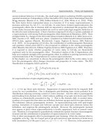
Fig. 8. Average ergodic capacities of the cellular MIMO systems using FRF 3 scheme and the
hybrid frequency reuse scheme.
Cellular MIMO Systems

201
Remark: As we know, the coverage problem (the transmission between the BS and MS fails
at the cell boundary due to the co-channel interference) has been the major problem for the
commonly used single-frequency-reuse cellular systems. From the numerical results, it is
seen that such problem can be greatly alleviated by using the proposed hybrid frequency
reuse scheme.
6. Conclusions
In this chapter, the downlink capacity of cellular MIMO systems has been theoretically
analyzed in terms of both ergodic and outage capacities. The FRF has been considered and a
hybrid frequency reuse scheme has been introduced. Numerical results have shown that
both the ergodic and outage capacities can be increased by the hybrid FRF scheme.
Especially, when compared with the commonly used FRF 1 scheme, the outage capacity can
be increased as much as 50%. Therefore, the hybrid FRF scheme can greatly alleviate the
coverage problem of the single-frequency-reuse cellular systems.
7. Reference
[1] V. Tarokh, N. Sehadri and A. R. Calderband, “Space-time codes for high data rate
wireless communication: Performance criterion and code constructions,” IEEE
Transactions on Information Theory, vol. 44, pp. 744-765, March 1998.
[2] G. J. Foschini, “Layered space-time architecture for wireless communication in a fading
environment when using multielement antennas,” Bell Labs Technical Journal, pp.
41-59, Autumn 1996.
[3] G. J. Foschini and M. J. Gans, “On limits of wireless communications in a fading
environment when using multiple antennas,” Wireless Personal Communications,
vol. 6, pp. 311-335, 1998.
[4] E. Telatar, “Capacity of multi-antenna Gaussian channels,” European Transactions on
Telecommunications, vol. 10, pp. 585-595, November 1999.

[5] M. S. Alouini and A. J. Goldensmith, “Area spectral efficiency of cellular mobile radio
systems,” IEEE Transactions on Vehicular Technology, vol. 48, pp. 1047-1066, July
1999.
[6] R. S. Blum, J. H. Winters and N. R. Sollenberger, “On the capacity of cellular systems
with MIMO,” IEEE Communications Letters, vol. 6, pp. 242-244, June 2002.
[7] W. Matthew, B. Mark and N. Andrew, “Capacity limits of MIMO channels with co-
channel interference,” IEEE Vehicular Technology Conference, pp. 703-707, 2004.
[8] M. M. Matalgah, J. Qaddour, A. Sharma and K. Sheikh, “Throughput and spectral
efficiency analysis in 3G FDD WCDMA cellular systems,” IEEE Globecom
conference, pp. 3423-3426, November 2003.
[9] S. Catreux, P. F. Driessen and L. J. Greenstein, “Simulation results for an interference-
limited multiple-input multiple-output cellular sysem,” IEEE Communications
Letters, vol. 4, pp. 334-336, November 2000.
[10] S. Catreux, P. F. Driessen and L. J. Greenstein, “Attainable throughput of an
interference-limited Multiple-Input Multiple-Output (MIMO) cellular systems ,”
IEEE Transactions on Communications, vol. 49, pp. 1307-1311, August 2001.
[11] K. Adachi, F. Adachi and M. Nakagawa, “On cellular MIMO spectrum efficiency,” IEEE
Vehicular Technology Conference, pp. 417-421, October 2007.
MIMO Systems, Theory and Applications

202
[12] Y. J. Choi, C. S. Kim and S. Bahk, “Flexible design of frequency reuse factor in OFCDM
cellular networks,” IEEE International Conference on Communications, pp. 1784-
1788, May 2006.
[13] T. M. Cover and J. A. Thomas, Elements of information theory, New York: Wiley, 1991.
[14] J. G. Proakis, Digital Communications, New York: McGraw Hill, 2001.
[15] Z. Wang and R. S. Gallacher, “Frequency reuse scheme for cellular OFDM systems,”
IEEE Electronics Letters, vol. 38, pp. 387-388, April 2002.
[16] Wei Peng and Fumiyuki Adachi, “Hybrid Frequency Reuse Scheme for Cellular MIMO
Systems,” IEICE Transactions on Communications, vol. E92-B, May 2009.

Part 3
Pre-processing and Post-processing
in MIMO Systems

9
MIMO-THP System with Imperfect CSI
H. Khaleghi Bizaki
Electrical and Electronic Engineering University Complex (EEEUC), Tehran,
Iran
1. Introduction
In recent years, it was realized that designing wireless digital communication systems to
more efficiently exploit the spatial domain of the transmission medium, allows for a
significant increase of spectral efficiency. These systems, in general case, are known as
Multiple Input Multiple Output (MIMO) systems and have received considerable attention
of researchers and commercial companies due to their potential to dramatically increase the
spectral efficiency and simultaneously sending individual information to the corresponding
users in wireless systems.
In MIMO channels, the information theoretical results show that the desired throughput can
be achieved by using the so called Dirty Paper Coding (DPC) method which employs at the
transmitter side. However, due to the computational complexity, this method is not
practically used until yet. Tomlinson Harashima Precoding (THP) is a suboptimal method
which can achieve the near sum-rate of such channels with much simpler complexity as
compared to the optimum DPC approach. In spite of THP's good performance, it is very
sensitive to erroneous Channel State Information (CSI). When the CSI at the transmitter is
imperfect, the system suffers from performance degradation.
In current chapter, the design of THP in an imperfect CSI scenario is considered for a
MIMO-BC (BroadCast) system. At first, the maximum achievable rate of MIMO-THP system
in an imperfect CSI is computed by means of information theory concepts. Moreover, a
lower bound for capacity loss and optimum as well as suboptimum solutions for power
allocation is derived. This bound can be useful in practical system design in an imperfect

CSI case.
In order to increase the THP performance in an imperfect CSI, a robust optimization
technique is developed for THP based on Minimum Mean Square Error (MMSE) criterion.
This robust optimization has more performance than the conventional optimization method.
Then, the above optimization is developed for time varying channels and based on this
knowledge we design a robust precoder for fast time varying channels. The designed
precoder has good performance over correlated MIMO channels in which, the volume of its
feed back can be reduced significantly.
Traditionally, channel estimation and pre-equalization are optimized separately and
independently. In this chapter, a new robust solution is derived for MIMO THP system,
which optimizes jointly the channel estimation and THP filters. The proposed method
provides significant improvement with respect to conventional optimization with less
increase in complexity.
MIMO Systems, Theory and Applications

206
Notation: Random variables, vectors, and matrices are denoted by lower, lower bold, and
upper bold italic letters, respectively. The operators E(.), diag(.),
⊥
, PDF, and CDF stand for
expectation, diagonal elements of a vector, statistically independent, Probability Density
Function, and Cumulative Distribution Function, respectively.
2. MIMO-BC-THP systems
2.1 Type of MIMO channels
There are three types system can be modeled as MIMO channel [1]:
a. point-to-point MIMO channel
This type of MIMO system is a multiple antenna scenario, where both transmitter (TX) and
receiver (RX) use several antennas with seperate modulation and demodulation for each
antenna. We refer this type of channel as MIMO channel (Central transmitter and receiver).
b. multipoint-to-point MIMO Channel

The uplink direction of any multiuser mobile communication system is an example of a
MIMO system of this type. The joint receiver at the base station has to recover the individual
users’ signals. We will refer to this type of channel as the MIMO multiple access channel
(Decentralized transmitters and central receiver).
c. point-to-multipoint MIMO Channel
The downlink direction of mobile multiuser communication systems is an example of what
we call a MIMO broadcast channel (Central transmitter and decentralized receivers).
2.2 Precoding strategy
The main difficulty for transmission over MIMO channels is the separation or equalization
of the parallel data streams, i.e., the recovery of the components of the transmitted vector
x
which interfere at the receiver side. The most obvious strategy for separating the data
streams is linear equalization at the receiver side.
It is well-known that linear equalization suffers from noise enhancement and hence has poor
power efficiency [2]. This disadvantage can be overcome by spatial decision-feedback
equalization (DFE). Unfortunately, in DFE error propagation may occur. Moreover, since
immediate decisions are required, the application of channel coding requires some clever
interleaving which in turn introduces significant delay [2].
The above methods require CS) only at the receiver side. If CSI is (partly) also available at
the transmitter, the users can be separated by means of precoding. Precoding, in general
case, stands for all methods applied at the transmitter that facilitate detection at the receiver.
If a linear transmitter preprocessing strategy is used, we prefer to denote it as
preequalization or linear precoder. In other case we refer it as non-linear precoder.
In MIMO channels a version of DFE by name, matrix DFE is used where is a non-linear
spatial equalization strategy at the receiver side. The feedback part of the DFE can be
transferred to the transmitter, leading to a scheme known as THP. It is well known that
neglecting a very small increase in average transmit power, the performance of DFE and
THP is the same, but since THP is a transmitter technique, error propagation at the receiver
is avoided [3]. Moreover, channel coding schemes can be applied in the same way as for the
ideal additive white Gaussian noise (AWGN) or flat fading channel.

The analogies between temporal equalization methods (in Single Input Single Output (SISO)
channels) and their direct counterparts as spatial equalization methods (in MIMO channels)
are depicted in Table I [2].
MIMO-THP System with Imperfect CSI

207


ISI channel
)(zH

(temporal Equalization)
MIMO channel
H
(spatial Equalization)
at Rx
Linear equalization via
)(/1 zH
Linear equalization via
1−
t
H
at Tx
Linear pre-equalization via
)(/1 zH

Linear pre-equalization via
1−
r
H

linear
at Tx / Rx OFDM/DMT, vector precoding SVD
at Rx DFE Matrix DFE

Non-linear
at Tx / Rx THP MIMO-THP
Table 1. Corresponding Equalization Strategies for ISI Channels and MIMO Channels.
2.3 The Principle of THP
The information theory idea behind the THP is based on Costa’s “writing on dirty paper
result” for interference channels [4], which can be informally summarized as follows:
"When transmitting over a channel, any interference which is known apriori to the transmitter does
not affect the channel capacity. That is, by appropriate coding, transmission at a rate equal to the
capacity of the channel without this interference is possible."
If we extend the Costa precoding concepts for multiple antenna with Co-Antenna
Interference (CAI) then THP structure can be obtained [1, 3]. Consider these subchannels in
some arbitrary order. In this case, the encoding for the first subchannel has to be performed
accepting full interference from the remaining channels, since at this point the interference is
unknown. For the second subchannel, however, if the transmitter is able to calculate the
interference from the first subchannel, “Costa precoding” of the data is possible such that
the interference from the first subchannel is taken into account. Generally, in the k
th

subchannel considered, Costa precoding is possible such that interference from subchannels
1 to k-1 is ineffective.
We can apply this result to the MIMO channel [5]: If the precoding operation contains a
Costa precoder, no interference can be observed from lower number subchannels into
higher number subchannels.

Note that it is possible to transform H into a lower triangular matrix with an orthonormal
operation [6]. In this way interference from lower-index subchannels into higher-index
subchannels is completely eliminated, and together with Costa precoding adjusted to this
modified transmission matrix, effectively only a diagonal matrix remains for the
transmission. It turns out that a simple scheme for Costa precoding works analog to the
feedbackpart of DFE, now moved to the transmitter side and with the nonlinear decision
device replaced by a modulo-operation. This is also known as THP [7, 8], and the link
between THP and Costa precoding was first explored in [9].
2.4 MIMO-THP system model
The base station with
T
n transmit antenna and
R
n user (in which
RT
nn
≤
) with single
antenna can be considered as MIMO broadcast system. A block diagram of this MIMO
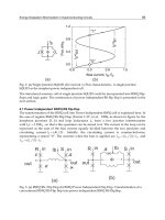
system together with THP is illustrated in Fig. 1 and is briefly explained here.
The
T
n dimensional input symbol vector a passes through feedback filter B , which is
added to the intended transmit vector to pre-eliminate the interference from previous users.
MIMO Systems, Theory and Applications

208

Fig. 1. THP model in a MIMO system
Then the resultant signal is fed to modulo-operator, which serve to limit the transmit power.

The output signal of modulo-operator is then passed through a feed forward filter to further
remove the interference from future users [10]. Finally, the precoded signal is launched in to
the MIMO channel. As all interferences are taken care of at the transmitter side, the receivers
at the mobile user side are left with some simple operations including power scaling
(diagonal elements of matrix G ), reverse modulo-operation, and single user detection.
According to Fig. 1, the base band received signal can be modeled as:
nxHr
+
=
~
(1)
where
1n
T
~
×
∈Cx
,
1n
R
×
∈Cr ,
T
n
CH
×
∈
R
n
and

1n
R
×
∈Cn are transmitted, received, channel and
noise matrices, respectively ( C denotes complex domain). The elements of the noise vector
are assumed as independent complex Gaussian random variables with zero mean and
variance
2
σ
, i.e., ),0(~
2
R
n
CΝ I
σ
n . The elements of matrix H are considered as complex
Gaussian random variables (i.e. flat fading case). In other words, the channel tap gain from
transmit antenna
i to receive antenna
j
is denoted by
ji
h which is assumed to be
independent zero mean complex Gaussian random variables of equal variance, that is
1]|[|
2
=
ji
hE .
The operation of THP is related to the employed signal constellation

A . Assume that in each
of the parallel data streams an
M
-ary square constellation (
M
is a squared number) is
employed where the coordinates of the signal points are odd integers, i.e.,
)}}1(31{{ −±±±∈+= M, ,,a,a|jaa
QIQI
A
. Then the constellation is bound by the square
region of side length
Mt 2= which is needed for modular operation [3].
Note: In the rest of the chapter, for means of simplicity, the number of transmit and receive
antennas are assumed to be the same (i.e.,
Knn
RT
=
=
). Also, we consider the flat fading
case. Whenever these assumptions are not acceptable we clarify them.
The lower triangular feedback matrix
B , unitary feed forward matrix F and diagonal
scaling matrix
G can be found by ZF or MMSE criteria as [11]. The received signal before
modulo reduction can be given as:
nvGHFBGry
~
1
+==

−
(2)
where
Gnn =
~
,and dav
+
=
is effective input data, and d is the precoding vector used to
constrain the value of
x
~
[13]. If ZF criterion is used, it requires IGHFB =
−1
. Thus, the
(.)
t
Γ
I-B
H
(.)
t
Γ
x
n
z

y
G
a

r
F
x
~
I-B
x
v
d
a
Linear Model
MIMO-THP System with Imperfect CSI

209
processing matrices
G , B , and F can be found by performing Cholesky factorization of
HH
H
as [13]:

RHF
GRB
diagG
RRHH
HH
1
)(
−
−−
=
=

=
=
1
KK
1
11
r, ,r
(3)

where ][
ij
r=R is a lower triangular matrix. The error covariance matrix can be shown as:

]/, ,/[diag]))([(E
222
11
2
~~
KKnn
H
nn
GnGn rσrσ==Φ (4)
i.e, the noise is white.
If MMSE criterion is used the matrix R can be found through Cholesky factorization of [5]:

RRIHH
HH
=+ )(
ζ
(5)

where
22
/
an
σσ=
ζ
. The matrices G , B and F can be found as:

HH
KK
HRF
GRB
G
−
−−
=
=
= ], ,[diag
11
11
rr
(6)
The error covariance can be shown as:
]/, ,/[][E
222
11
222
KKnnn
H
ee

diagGee rσrσσ ===Φ (7)

i.e. error can be considered as white.
In outdated CSI case, the system model, which is considered in Fig. 1, operates in a feedback
channel where the CSI is measured in downlink and fed to the transmitter in uplink
channel. Time variations of channel lead to a significant outdated (partial) CSI at the
transmitter. In fact there will always be a delay between the moment a channel realization is
observed and the moment it is actually used by the transmitter. The effect of time variations
(or delay) can be considered as:
HHH Δ+=
ˆ
, where
HH
ˆ
,
and
HΔ
are true, estimated and
channel error due to time variations [13]. We assume that the channel error has Gaussian
probability density function with moments
0][
=
Δ
HE and
H
H
CHHE
Δ
=ΔΔ ].[ .
According to Fig. 1, the received signal can be considered as:

nvFBHHGGry
~
)
ˆ
(
1
+Δ+==
−
(8)

where Gnn =
~
and
v
is effective data vector [12]. If ZF criterion is used, it requires:
IFBHG =
−1
ˆ
(9)
The processing matrices
BGR ,, and F can be found by doing Cholesky factorization of
H
HH
ˆˆ
as [11]:
MIMO Systems, Theory and Applications

210

RHF

GRB
G
RRHH
KK
HH
1
11
11
ˆ
), ,(
ˆˆ
−
−−
=
=
=
=
rrdiag
(10)
where
GnHFxGnwe
+
Δ
=+=
~
is considered as an error vector and the term w stands for
channel imperfection effect due to outdated CSI. The error covariance matrix can be
obtained as:

H

Hx
H
ee
GICGeeE )(][
2
ζσ
+==Φ
Δ
(11)
Note that, with a small channel error assumption (i.e.
0→
ΔH
C ), the error covariance matrix
in an imperfect case tends to the error covariance matrix in a perfect case, i.e.

)/1, ,/1,/1(
2 2
KK
2
22
2
11
rrrDiag
xee
σ
=Φ (12)
3. MIMO-THP capacity
The first attempt to calculation of achievable rates of THP is done by Wesel and Cioffi in
[15]. The authors considered THP for discrete-time SISO consists of Inter-Symbol
Interference (ISI) and AWGN. They derived an exact expression for maximum achievable

information rate for ZF case and provided information bound for MMSE case. In this
section, we develop the achievable rates analysis provided in [15] for MIMO-THP in flat
fading channel. We obtain the maximum achievable rate and some upper and lower bounds
of it for ZF and MMSE cases with perfect and imperfect CSI.
3.1 Achievable rates of point-to-point MIMO-THP
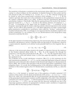
Consider a point-to-point MIMO system with THP as Fig. 2.


(.)
t
Γ
I-B
H
(.)
t
Γ
x
n
z
y
GF
a
r


Fig. 2. THP model in a point-to-point MIMO system
The received signal vector can be expressed as:

[
]

ΓΓ
1
[]
−
′
=+=++
tt
azGFHBvGFn wn (13)
where
w is residual spatial interference after MMSE criterion on THP filters (in the ZF case
0=w ) and
(.)
t
Γ
is modulo
t
operator so eliminate its output on interval
)2/,2/[)2/,2/[
kkkk
jtjtttT
−
×−= . As GFnn
=
′
is white Gaussian noise and with the
MIMO-THP System with Imperfect CSI

211
assumption that
jiji

waww
⊥
⊥
& for ji
≠
∀
(so that symbol
⊥
stand for statistical
independence) the received vector r can be decoupled in K parallel streams as
1
[17]:

[
]
Kknwaz
kkktk
~1; =
′
++Γ= (14)
Because of the decoupling of the received information symbols in (14) and assuming
independence between elements in a the mutual information between the transmitted
symbols and the received signal vector can be expressed as the sum of the mutual
information between elements of each vector:

() ( )
∑
=
=
K

k
kk
zaII
1
;za; (15)
where
(.)I denote mutual information. Each term in the sum is independently can be
considered as:

()
(
)
(
)
(
)
(
)
()
[]
()
[]
kkktkkkt
kkkktkkktkkkkk
anwhnwah
anwahnwahazhzhzaI
|)(
]|)([][|;
′
+Γ−

′
++Γ=
′
++Γ−
′
++Γ=−=
(16)
where
(.)h
denotes differential entropy. Calculation of the above mutual information seems
to be difficult and we try to find an upper and lower bound of (16) by some approximations.
Remark 1: An upper bound on the achievable rate of the channel produced by MMSE-THP of
(16) can be found as [17]:

() ()
[
]
(
)
∑
=
′
Γ−=
K
k
ktUpper
nhtI
1
2
)(log2za;

(17)
Also, the upper bound can be obtained essentially by neglecting the spatial interference
term
k
w in (16) [17]. The lower bound depends largely on the variance of
k
w [15]. A lower
bound on achievable rate can be found as [17]:

()
))2/(2(log2log)2(log)(log2
2
1
2
2
2
2
22
σ
σ
γ
πσ
terfetI
K
k
Lower
−−−=
∑
=
za; (18)

Thus, a truncated Gaussian [17] with variance of
(
)
)(var
2
ktk
nw
′
Γ+=
γ
produces a slightly
tighter bound but requires the computation of
(
)
)(var
kt
n
′
Γ
.
Remark 2: The upper bound attained in (17) can be simplified if some approximations are
allowed so that a quasi-optimal (or sub-optimal) closed form solution can be found. This
approximations can be done based on the value of
σ
/t (See [17]).
3.2 General THP in point-to-point MIMO with perfect CSI
Whenever CSI is available at the transmitter in a communication system, since the
transmitter has knowledge of the way the transmitted symbols are attenuated and
distributed by the channel, it may adjust transmit rate and/or power in an optimized way.

1
For MMSE case the above assumption for high value of SNR is acceptable and the above results can be
true in asymptotic case, so MMSE performance for high SNR values converge to ZF [2].
MIMO Systems, Theory and Applications

212
For instance, in the multi-antenna scenario some of the equivalent parallel channels might
have very bad transmission properties or might not be present at all. In this situation, the
transmitter might want to adjust to that by either dropping some of the lower diversity
order sub channels or by redistributing the data and the available transmission power to
improve the average error rate. This can be done by generalization of THP concepts as
GTHP by enabling different power transmission for each antenna. GTHP can be done in two
main scenarios [17]:
First: If the loading is made according to capacity of system; this structure enables different
transmission rate per antenna.
Second: If it is needed to ensure reliable transmission rate for each antenna, the loading
should be made according to minimize error rate of system.
Here we consider two different optimization scenarios for loading strategies of THP and
extend it's concept in structure that t is not constant, so the modulo interval is different for
each sub channel (
k
t ) [17].
3.2.1 Capacity criterion
In this section, the power adaptation strategy of the second type of GTHP concept is
employed. The optimal power allocation is calculated in MIMO-GTHP systems, while
regarding the modulation schemes is given. If the loading is made according to capacity of
system, this structure enables different transmission rate per antenna. One of the good
features of this scenario is that it is scalable architecture, because it allows adding or
removing transmitters without losing the precoding structure as explained in [16].
If

a assumed as an i.i.d. uniform distribution on T, for such a case,
x
is also i.i.d. uniform
on T (regardless of the choice of matrix
B
). Thus the transmitted power from k
th
antenna
will be
6/}|{|
22
kkk
txEp == (for real case 12/
2
kk
tp = ). Its corresponding rate will equal the
maximum achievable mutual information in (17):

(
)
)]([)(log2,;)(
2 ktkkkkk
nhttzaItI
k
′
Γ−==
(19)
Then the maximum achievable rate for a system with THP will be the maximum of the sum
of the rates of each stream subject to a maximum total transmitted power constraint, i.e.

{} {}
⎪
⎪
⎩
⎪
⎪
⎨
⎧
==
′
Γ−==
∑∑
∑∑
==
==
T
K
k
k
K
k
k
K
k
ktk
t
K
k
k
t

General
Ptpts
nhttIC
k
kk
1
2
1
1
2
1
6
1

)])([)(log2(max)(max
(20)
In order to maximize (20) we assume that all the available streams are classified into two
groups
2
(
g
-Gaussian and u –uniform) based on
σ
/t values [16]. As shown in [17], the
achievable rate of streams belonging to
u tends to zero; no power is assigned to these
streams, i.e.
ukt
k
∈

∀
= 0 . Thus the solution of the maximization problem in (20) can be
found as assigning the same power to the entire stream in
g
(and no power to those in u ).
The optimal solution can be shown to be [17]:

2
Based on the value of
σ
/t
for each stream
MIMO-THP System with Imperfect CSI

213
gk
g
p
IC
gk
n
T
k
Adaptive
General
k
∈
⎟
⎟
⎠

⎞
⎜
⎜
⎝
⎛
=
∑
∈
,
6
2
'
σ
(21)
where
g
denotes the number of active antennas and
2
'
k
n
σ
is variance of
k
n' . Then some kind
of adaptive rate algorithm is necessary to achieve the maximum capacity of the GTHP.
3.2.2 Minimum SER criterion
In some application it is needed to ensure reliable transmission rate for each antenna
(especially in MIMO broadcast channels). In this section we try to find the optimal sub
channel power allocation in MIMO GTHP systems, while regarding the modulation

schemes is given. As mentioned, for each sub channel we have:
K1,2, ,kn'az
kkk
=
+
=
(22)
where we assumed that
k
w tend to zero. For simplicity assume MQAM transmission in all
sub channels is used. In this case the approximate average SER for a fixed channel
H

simply given as [17]:

∑
=
−
−≈
K
1k
k
2
n'
2
kk
k
k
E
σ

r
M
Q
M
SER )
1
3
()
1
(1
(23)
where
k
2
kk
k
k
M
r
M
B
1
3
−
=
and we assumed modulation order (i.e.
k
M ) can be varied for each
sub-channel, so that variable bit allocation is possible (that we didn't consider here). In this
case we have [17]:

)( Λ
A
B
W
B
1
E
k
k
k
k
= (24)
where
2
2
(1)
(1)
−
=
−
kk
k
kkk
MM
A
Mr
and )(xW is the real valued Lambert’s W -function defined as
the inverse of the function 0;.)( ≥= xexxf
x

, i.e., xa.eaxW
a
=⇔=)( .
Since the
)(xW function is real and monotonically increasing for real ex /1
−
> , the value of
λ
such that 0KE
K
1k
k
=−
∑
=
)(
λ
holds which can be found by using some classical methods as
denoted in [17]. On the other hand, )(xW is a concave and unbounded function with
0W(0) = and xxW
≤
)( , the unique solution for
T
K
EE ], ,[
1
=E can be found by the
following simple iterative procedure[14]:
i. Chose a small positive
Λ

which satisfy

T
K
1k
k
E
A
Λ
≤
∑
=
(25)
ii. Calculate
MIMO Systems, Theory and Applications

214

∑
=
=
K
1k
k
k
k
T
Λ)
A
B

W(
B
1
E
ˆ
(26)
iii. If
T
E
ˆ
is not yet sufficiently close to
T
E , multiply
Λ
by
TT
E/E
ˆ
and go back to step (ii).
iv. Compute
T
K
EE ], ,[
1
=E according to (24).
Note that since )(xW for ex /1
−
> is monotonic function, then according to relation (24) the
highest power
)(max

k
E assign to the weakest signal so that the SNR value almost stay
constant for all sub channels.
3.3 Achievable rate in imperfect CSI
In [17] the scheme proposed in [18] for MIMO THP system was modified by allowing
variations of the transmitted power in each antenna. The authors stated the problem of
finding the maximum achievable rate for this modified spatial THP scheme and found that
Uniform Power Allocation (UPA) with antenna selection is a quasi-optimal transmission
scheme with a perfect CSI.
In this sub-section, based on previous researches about SISO and point-to-point MIMO
channels, an analytical approach to attain the maximum achievable rate bound in an
imperfect CSI case is developed for broadcast channel. It will be shown that this bound
depends on the variance of the residual Co-Antenna Interference (CAI) term. Moreover, it
will be shown that the power allocation obtained by the UPA in [17] is sub-optimal in an
imperfect CSI, too.
3.3.1 Maximum achievable rates
The received signal after modulo operation can be considered as
]
~
[ nHFxGaz
k
t
+
Δ
Γ
+
=
. Since
x
has i.i.d. distribution, HFxGW

Δ
=
can be considered as an unknown interference with an
i.i.d. distribution. Also, for such an
a ,
z
is i.i.d. uniform on
T
. In this case, the received
information can be decoupled in
K
independent parallel data steams and the mutual
information between
th
k element of data vector,
k
a , and the corresponding element of the
received signal,
k
z , is [13]:

()()( )() ( )
⎥
⎥
⎦
⎤
⎢
⎢
⎣
⎡

⎟
⎟
⎠
⎞
⎜
⎜
⎝
⎛
+
′
Γ−≤+Γ−=−=
∑
=
kj
K
j
kk
kj
tkkkktkkkkkk
nx
r
hpanwhzhazhzhzaI
kk
~
)6(log]|)
~
([|;
1
2
δ

(27)
where
kjkj
][ HFΔ=
′
δ
and (.)h denotes differential entropy. Let us define the random variable
k
e as
kj
K
j
kk
kj
k
nx
r
e
~
1
+
′
=
∑
=
δ
where its power is
∑
=
+=

K
j
kj
kk
j
kk
n
ek
r
p
r
1
2
22
2
2
δ
σ
σ
and
kjkj
H ][
Δ
=
δ
. With the
assumption of small error,
k
e can be approximately modeled as a complex Gaussian
random variable. In the case where, the above assumption is true, the mutual information

expression (27) can be very well approximated as [13]:

(
)
[
]
+
≈
kkk
zaI
χ
2
log;
(28)
where
MIMO-THP System with Imperfect CSI

215

⎪
⎩
⎪
⎨
⎧
=
+=
+
=
∑
]0),max[log(]log[

)(/6
1
2
22
xx
pepr
K
j
jkjnkkkk
δσπχ
(29)
The achievable rates for THP in an imperfect CSI case will then be the sum of the mutual
information of all
K
parallel steams as [13]:

[]
2
{} {}
11
1
max ( ; ) max log

+
==
=
⎧
=≈
⎪
⎪

⎨
⎪
=
⎪
⎩
∑∑
∑
kk
KK
kk k
pp
kk
K
kT
k
CIaz χ
st p P
(30)
Observed that C (or
k
χ
) depends on three components:
2
2
,
kkkj
r
δ
and
k

p . In order to
maximize
k
χ
, some kind of spatial ordering is necessary in order to maximize it. For this
purpose, it is required to decompose H (in Cholesky factorization) so that the elements of
2
kk
r to be maximized (finding the ordering matrix similar to [11]).
On the other hand, it was assumed that by making small error assumption,
k
e can be
approximately modeled as a complex Gaussian random variable. This is equivalent to
assuming
jp
njkj
j
∀≤ ;||max
22
σδ
. Now, we assume that the entries of error matrix are
bounded as jk
kjkj
jk
,;||max
2
,
∀≤
αδ
[13]. In addition, for the sake of simplicity and without

loss of generality, we assume that
kj
jk
α
α
,
max
=
. Then, the power distribution that will
maximize the achievable rates will be the solution of the following maximin problem:

[]
⎪
⎪
⎩
⎪
⎪
⎨
⎧
∀≤=
=
∑
∑
=
=
+
jippts
C
ij
ji

T
K
k
k
K
k
k
p
iji
,;max,
logminmax
2
,
1
1
2
αδ
χ
δ
(31)
In order to solve the above maximin problem the worst-case is assumed, i.e.
ji
ij
ji
,;||max
2
,
∀=
δα
. With this assumption, the minimum mutual information will be

attained for each term in the summation. Then, the resulting maximization problem leads to
[13]:

⎪
⎪
⎩
⎪
⎪
⎨
⎧
=
⎥
⎦
⎤
⎢
⎣
⎡
+
=
∑
∑
=
=
+
T
K
k
k
K
k

Tn
kkk
p
ppts
pe
rp
C
i
1
1
2
2
2

)(
6
logmax
ασπ
(32)
The resulting maximization problem is a standard constrained optimization problem, and
can be solved with the use of the Lagrange method in which the solution result is .constp
k
=
It means that the
k
p
is independent of k , i.e the distribution of the power, in worst-case, is
UPA.
MIMO Systems, Theory and Applications

216
Note that, if we consider different noises with different powers for each user, the
distribution of power may not be the UPA.
3.3.2 Capacity loss
In the previous section, it is shown that the capacity of MIMO-THP can be obtained by the
UPA. More over, it can be observed from (32) that this capacity, in worst case, depends on
the channel error value (i.e.
α
). We define the capacity loss as difference between the
capacity of MIMO-BC-THP in a perfect CSI and in an imperfect CSI, i.e. relation (32), as [19]:

[]
KK
pe
rp
e
rp
CCC
K
k
Tn
kkk
K
k
n
kkk
+≤
⎥
⎦
⎤

⎢
⎣
⎡
+
−
⎥
⎦
⎤
⎢
⎣
⎡
=−=Δ
∑∑
==
1log
)(
6
log
6
log
ˆˆ
2
1
2
2
2
1
2
2
221

ασπσπ
(33)
The above bound for capacity loss only is valid for values of
α
so that the approximation of
jp
njkj
j
∀≤ ;||
22
max
σδ
is valid [19]. It means that this bound depends on SNR value and is
acceptable for high SNR value, i.e., this capacity loss bound is asymptotic bound for worst-
case in which bounds the capacity loss of MIMO-THP . It is desired to bounding the capacity
loss of optimal solution of (29). Assume
2
C
is the capacity of optimal solution that can be
obtained by exactly analysis or by numerical simulation. In this case we can bound
21
CCC −=Δ
as [19]:

[]
εα
σ
+
⎥
⎥

⎦
⎤
⎢
⎢
⎣
⎡
⎟
⎟
⎠
⎞
⎜
⎜
⎝
⎛
+−+=Δ
2
22
1log1log
n
T
p
KKKC
(34)
where
ε
is a positive value. The lower bound can be obtained by choosing 2−
=
K
ε
[19]:

[]
+
⎥
⎥
⎦
⎤
⎢
⎢
⎣
⎡
−+
⎥
⎥
⎦
⎤
⎢
⎢
⎣
⎡
⎟
⎟
⎠
⎞
⎜
⎜
⎝
⎛
+−+≥Δ )2(1log1log
2

22
K
p
KKKC
n
T
α
σ
(35)
where
]0,max[][ xx =
+
. In simulation we refer (35) as theoretic loss.
3.4 Spatial ordering
The VBLAST-Like ordering can be used in order to improve the power loading performance of
MIMO-GTHP system in Fig. 1 [1]. To do this, since the loading is based on the SNR values of
the equivalent parallel sub-channels, which in turn are proportional to
2
kk
r , the distribution of
these diagonal entries is an essential parameter in power loading performance. It turns out that
by introducing a permutation matrix in the decomposition of H, i.e, allowing different
ordering of the sub channels, the distribution of the
2
kk
r values can be modified as [1]:
)(minarg)||/1, ,||/1,||/1(minarg
2
22
22

2
11
GP
PP
==
KKopt
rrr
It means that in the cholesky factorization of (4), the decomposition should be made so that
the square value of diagonal elements of matrix R minimized. It means that the matrix P is
selected so that the column of H corresponding to minimum square value of diagonal
elements of G is permuted to the left. Deleting this column from the matrix H, and forming
MIMO-THP System with Imperfect CSI

217
the cholesky factorization of this modified matrix, we can obtain second column of matrix P.
Continuing this way, constantly updating P, the decomposition of H is constructed. The
pseudo-code for the algorithm is given in Fig. (3).

end
))(zeros(size=
1=P
)(g minarg= l
))^2diag(inv(=
MMSEfor;)chol(=
ZFfor;)qr(] [
:doKto1=i for
0][p=
:tionInitializa
ii
i

l:,l:,
i,l
ji,
j
i
H
i.j
HH
RG
IHHR
HRQ
P
ζ
+
=
=

Fig. 3. The pseudo code for ordering
Note that for ZF or MMSE-THP, the system performance will be dominated by the signal
component with the largest noise variance, and we can find the ordering algorithm in the
minimax noise variance sense as [1].
3.5 Simulation and results
3.5.1 Perfect CSI
The mutual information for real
k
x
with i.i.d uniform distribution on the module interval [-
t/2, t/2) is plotted in fig. 4, where the average transmitter energy is
12/
2

t . This figure also
shows the mutual information curves for the upper (17) and lower (18) bounds for each sub
channel. For comparison we also plotted the well-known AWGN channel capacity (with no
ISI). Observe that the upper bound lies above the AWGN capacity and lower bound lies
below this capacity (especially for high SNR values).
Figs. 5 and 6 give the performance comparison of the MMSE-GTHP with/without power
loading (relation (24)) when 4QAM and 16QAM modulations are used, respectively. From
these figures, it is clearly seen that the MMSE-GTHP with ordering can achieve better
performance than the MMSE-GTHP with or without power allocation (4QAM or 16QAM,).
When 4QAM modulation is used, at BER=2×10
-4
we can observe that the MMSE-GTHP with
power allocation achieves about 7dB gain, while this structure with power loading and
ordering gives about 11.5dB gain. When 16QAM is used, at BER=5×10
-4
the MMSE-GTHP
with power allocation gives approximately 6.5dB gain, while this structure with power
loading and ordering gives about 10dB gain. As can be seen from these figures, the
performance of power loading is noticeable, especially when it combined with sub-channel
ordering.
3.5.2 Imperfect CSI
For simulation purposes we have considered K=4 users. The entries of
H
ˆ
and
HΔ
have
been assumed to be zero mean i.i.d. complex Gaussian random variables, i.e.,
)1,0(~
ˆ

CNH
MIMO Systems, Theory and Applications

218

Fig. 4. Upper and lower bound of mutual information

Fig. 5. Performance comparison of MMSE-GTHPwith power loading and ordering for
4QAM.

Fig. 6. Performance comparison of MMSE-GTHP. with power loading and ordering for
16QAM
MIMO-THP System with Imperfect CSI

219

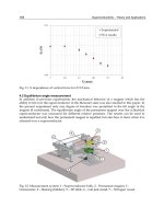
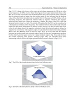
Fig. 7. Validation of approximation of
α


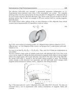
Fig. 8. Capacity with K=4 user and different value of
α


Fig. 9. Capacity loss for K=4 user
MIMO Systems, Theory and Applications

220

Fig. 10. Capacity loss for different user and 05.0

=
ρ

and
),0(~
2
ρ
CNHΔ . The validity of the approximations of (
jp
nj
∀≤ ;
2
σα
) for
dBP
nT
16/
2
=
σ
is shown in Fig. 7 by plotting the fraction of channel realizations in which the
approximations are valid for different values of
α
. The simulation is done for more than 10
4

channel realization and the validity is calculated as the number of iteration where the
inequality is valid. It can be seen that, for the particular values of the simulation parameters
taken in this section, the capacity analysis is valid for values of
α

up to −10 dB. In Fig. 8, we
have plotted the mean of the maximum achievable rates for the UPA scheme for different
values of
α
. It can be seen that for values of 01.0
≤
α
the capacity loss due to the presence of
channel errors are negligible and by increasing the SNR value, the capacity increases up to a
constant value. It means that by increasing the SNR value the capacity remains almost
constant. Figs. 9 and 10 depict asymptotic capacity loss in a time varying channel for
different values of
ρ
and different users, respectively. It can be seen that the attained
aproximated bound is valid for variety of rang of the channel errors and number of users,
especially for high SNR value (asymptotic case).
4. Robust MIMO-THP
4.1 Design criterion
The error, that is needed to be considered for the system illustrated in Fig. 1, should be the
difference between the effective data vector
v
and the data vector entering the decision
module
y
, i.e.:

nxBFHHGvye
~
])
ˆ

([ +−Δ+=−= (36)
The MMSE solution should minimize the error signal as:

⎪
⎩
⎪
⎨
⎧
≤
+−Δ+
T
GFB
x
nxBFHHG
PEs.t.
E
2
2
,,
~
~
])
ˆ
([minarg
(37)
MIMO-THP System with Imperfect CSI

221
Instead of solving (37), it is easier to use the orthogonallity principle [1]. In this case, the
MMSE solution should satisfy:

0][E =
H
er (38)
Thus, according to (36) we have:

xrrr
BG Φ=Φ
(39)
The matrices
rr
Φ and
xr
Φ
can be computed by using (36) as [13]:
)
ˆˆ
(][E
2
H
H
x
H
rr
CIHHrr
Δ
++==Φ
ζσ
(40.a)

HH
x
H
xr
HFxr
ˆ
][E
2
σ
==Φ (40.b)
where
22
/
xn
σσζ
= . Substituting relation (40) for (39) and some manipulation, yielding [13]:

H
H
HH
HCIHHGBF
−
Δ
−
++=
ˆ
)
ˆˆ
(
1

ζ
(41)
Since F is a unitary matrix [1]:

)
ˆˆ
(
ˆˆ
)
ˆˆ
(
1
H
HH
H
HH
CIHHHHCIHHRR
Δ
−−
Δ
++++=
ζζ
(42)
where
BGR
1−
= is assumed. The matrix R can be found through Cholesky factorization of
(42) and the matrices G, B, and F can be obtained as [13]:

H

H
H
KK
RCIHHHF
GRB
G
−
Δ
−
−−
++=
=
=
)
ˆˆ
(
ˆ
], ,[diag
1
11
11
ζ
rr
(43)
Using the B, F and G obtained in (43), the error covariance matrix can be computed as [13]:

H
H
H
x

H
ee
GCIHHGeeE )
ˆˆ
(][
122
Δ
−−
++==Φ
ζζσ
(44)
It means that the error covariance matrix in imperfect CSI is the sum of covariance matrix in
perfect CSI plus the term
H
Hx
GGC
Δ
2
σ
. This term tends to zero with low channel error
assumption (perfect CSI), i.e.:

HH
n
H
ee
GIHHGeeE )
ˆˆ
(][
12

+==Φ
−−
ζσ
(45)
In this case, R can be found through:

)
ˆˆ
(
ˆˆ
)
ˆˆ
(
1
IHHHHIHHRR
HHHH
ζζ
++=
−−
(46)
and the matrices G, B and F can be computed as:

HHH
KK
RIHHHF
GRB
G
−−
−
−

+=
=
=
)
ˆˆ
(
ˆ
], ,[diag
1
11
11
ζ
rr
(47)
MIMO Systems, Theory and Applications

222
The above results (45-47) are the same as [12], where it is assumed that the perfect CSI is
available. In this section, relations 45 to 47 are referred to as conventional optimization and
relations (42-44) are referred to as robust optimization.
4.2 Robust optimization with channel estimation consideration
4.2.1 Channel estimation
The received signal at the base station during training period (uplink) , at time stand i, can
be modeled as [13]:

)()()( iii naHy
T
+= (48)
During the training period of N symbols in uplink transmission, the received signal can be
constructed as [13]:

nshy
ss
+
=
(49)
where
T
s
Nyyy )]1(, ),0([ −= ,
T
Nnnn )]1(, ),0([ −= , ][vec
T
s
Hh = ,
T
NAAs )]1(, ),0([ −= ,
and A(i) can be constructed as block diagonal matrix with elements of a(i)
T
. Based on the
received signal in (49), the Best Linear Unbiased Estimator (BLUE) channel estimation can
be performed as [20]:

ss
HH
sn
H
n
H
s

WyysssyCssCsh ===
−−−− 1111
)()(
ˆ
(50)
with the covariance matrix of:

1211
ˆ
)()(
−−−
== sssCsC
H
nn
H
h
s
σ
(51)
4.2.2 Improved robust optimization
In the robust optimization, only THP filters were optimized according to the MMSE
criterion and the channel estimator was optimized separately from THP. Here, the above
solution is extended to optimize THP filters together with the channel estimator conditioned
on observed data. In this case, cost function should be optimized with respect to THP filters
and the observed data. Thus, the goal is to optimize the precoder directly based on the
available observation y
s
.

Based on the linear model of (49), the conditional PDF )|(

| ssyh
yhp
ss
is a complex Gaussian
process with moments ]|[E
| ssyh
yh
s
=
μ
and ]|))([(
||| s
H
yhsyhsyh
yhhEC
sss
μμ
−−= [18].
According to the Bayesian Gauss-Markov theorem, the Bayesian estimator can be written as
[20]:

sssn
H
h
H
hyh
yWyIssCsC
sss
=+=
−12

|
)(
σμ
(52)
and the covariance matrix of channel estimator is:

sss
hshyh
sCWCC −
=
|
(53)
where
][
H
ssh
hhEC
s
= . In order to optimize the THP filters, the cost function in the previous
section should be modified conditional to the observed data, i.e.:
MIMO-THP System with Imperfect CSI

223

]|[E
H s
H
ee
yee=Φ
(54)

By using the orthogonallity principle, the MMSE solution should be equivalent to:

0]|[E
H
=
s
H
yer (55)
As relation (39) it is possible to write [13],

ss
yxryrr
BG
||
Φ
=
Φ
(56)
Like the sub-section 4.1, the matrix R can be found through Cholesky factorization of [13]:

)
ˆˆ
(
ˆˆ
)
ˆˆ
(
|
1
|

ss
yh
HH
yh
HH
CIHHHHCIHHRR ++++=
−−
ζζ
(57)
and matrices G, B and F can be found as:

H
yh
H
KK
RCIHHHF
GRB
G
s
−−
−−
++=
=
=
)
ˆˆ
(
ˆ
], ,[diag
|

1
11
11
ζ
rr
(58)
In this case, the error covariance matrix has the form [13]:

H
yh
H
xee
GCIHHG
s
)
ˆˆ
(
|
122
++=Φ
−−
ζζσ
(59)

It means that the improved robust optimization can be done by replacing
H
C
Δ
in the robust
optimization with its equvalent, i.e.

s
yh
C
|
.
4.3 Power loading in imperfect CSI
In sub-section 3.4, we discussed about power loading of point-to-point MIMO-THP in
perfect CSI. Now we develop this power loading in MIMO-BC-THP for imperfect case.
4.3.1 Optimal solution
It is easy to approximate the SER of each sub-streams for imperfect CSI as [13]:

∑
=
−
−≈
K
1k
2
e
k
k
k
)
σ
p
1M
3
)Q(
M
1

(1SER
(60)
so
k
p is the power of transmitted symbols of k
th
user and from (59) we have,

⎟
⎠
⎞
⎜
⎝
⎛
++=Φ=
∑
=
k
K
j
kjjn
kk
kkee
2
e
p
r
σ
βδσ
1

2
2
2
1
][
(61)
where
ijij
][ HΔ=
δ
,
∑
=
=
K
j
jkjnk
ph
1
2
4
/
~
σβ
, and
ij
H
HH ]
ˆˆ
[

~
1−−
=
ij
h . Assuming small error in (61), i.e.
jp
nj
∀≤ ;
2
σα
,
2
e
σ can be approximated as [13]: