MIMO Systems Theory and Applications Part 10 ppt

0.01 0.02 0.03 0.04 0.05 0.06 0.07 0.08 0.09 0.1
10
-4
10
-3
10
-2
10
-1
10
0
e
2
Average Uncoded BER
SW-THP, N=2
Robust SW-THP, N=2
SW-THP, N=3
Robust SW-THP, N=3
15 20 25 30 35 40
10
-3
10
-2
10
-1
10
0
SNR (dB)
Average Uncoded BER
Stat. Robust THP,

Robust SW-THP,
Robust SW-THP,
=0.005
e
2
=0.01
e
2
=0.01
e
2
=0.005
e
2
Stat. Robust THP,
σ
σ


λ −

λ



λ

λ

≥




λ

λ




λ

λ




λ

λ

−


λ −

λ


≥ −




−

≥

−

· − −
−
−

Π F T R

Π
R F T
t

Π
F T R



Π F

T

R


F

T

Π R
Π R

F T
Π F T R Π R

Π
R


Π F

T

R

R
Π

Π

Π
Π Π

Π Π


Π
R



Π R


Π
R


Π F T R

R

Π
F T R



Π F T R


Π
F T R



Π F T R



−
−
11
Iterative Optimization Algorithms to
Determine Transmit and Receive Weights
for MIMO Systems
Osamu Muta, Takayuki Tominaga, Daiki Fujii, and Yoshihiko Akaiwa
Kyushu University
Japan
1. Introduction
As a technology to realize high data rates and high capacity in wireless communication
systems, Multiple-Input Multiple-Output (MIMO) system has received increasing attention.
In MIMO systems, high spectral efficiency is achieved by spatially multiplexing multiple
data streams at the same time and frequency [1].
The MIMO system with space division multiplexing (SDM) technique is categorized into
two cases, i.e., no channel state information (CSI) is needed at the transmitter or CSI is
exploited in both transmitter and receiver. As a method used in the former systems, spatial
filtering and maximum likelihood detection (MLD) are known [1], where the received SDM
signal is de-multiplexed with signal processing at the receiver. One of the latter MIMO
systems is called the Eigenbeam SDM (E-SDM) [1][2], where data streams are transmitted
through multiple orthogonal eigenpath channels between the transmitter and the receiver.
Thus, the E-SDM system with power control based on the water-filling theorem [3] improves
the MIMO channel capacity, provided that accurate CSI is known to the transmitter and the
receiver. Therefore, it is expected that the E-SDM system achieves significant increase of
spectral efficiency. In the E-SDM system, it is important to find optimum transmit and receive
weights for maximizing its capacity. Such the optimum weights are determined based on
eigenvector of H

H
H, where H denotes channel matrix and suffix H denotes complex conjugate
transpose. As a method to find these eigenvectors, eigenvalue decomposition (EVD) of H
H
H or
singular value decomposition (SVD) of H is well-known. Generally, SVD or EVD requires
matrix decomposition operation based on QR decomposition.
MIMO techniques can be used for multiple access systems where multiple signals are sent
from multiple terminals at the same time and same frequency, i.e., Space Division Multiple
Access (SDMA) or multi-user MIMO (MU-MIMO) [6]-[9]. When such a multi-antenna
system is used at a transmitter, the transmit weights are optimized under the constraint of
total transmit power [5]-[9]. However, the maximum transmit power for each antenna
element in SDMA systems is not restricted in general assumptions. Therefore, in the worst
case, an amplifier whose maximum output power is the same as total transmit power is
needed for each antenna element; these amplifiers cause an increase in cost. From this point
of view, it is desirable to use a reasonable (i.e., low cost) power amplifier for each antenna
element, where per-antenna transmit power is limited within a permissible output power.
MIMO Systems, Theory and Applications

266
To meet this requirement, it is necessary to determine weight coefficients so that the
transmit power for each antenna is limited below a given threshold.
In Ref.[10], a method to maximize transmission rate in eigenbeam MIMO-OFDM system
under constraint of the maximum transmit power for an antenna has been reported, where the
weights are determined by considering only the suppression of inter-stream interference (i.e.,
the optimum weights are first determined without considering the constraint of per-antenna
power, and then the total transmit power is normalized to meet the power constraint).
However, this method does not optimize weight coefficients in presence of noise and
interference. To find the optimum weights under per-antenna power constraint, these two
factors (inter-stream interference and signal-to-noise power ratio) have to be taken into

consideration simultaneously.
In this paper, first we propose an iterative optimization algorithm to find optimum transmit
and receive weights in an E-SDM system, where the transmitter is equipped with a virtual
MIMO channel and virtual receiver to obtain the optimum transmitter weight. The
transmitter estimates the optimum transmitter weights by minimizing the error signal at the
virtual receiver. Second, we propose an optimization method of transmit and receive
weights under constraints of both total transmit power and the maximum transmit power
for an antenna element in MU-MIMO systems, where the transmit weights are optimized by
minimizing the mean square error of the received signal to obtain the minimum bit error
rate (BER) under the per-antenna power constraint, provided that the knowledge of channel
state information (CSI) and the receive signal to noise power ratio (SNR) is given. In our
study, we solve this optimization problem by transforming the above constrained
minimization problem to non-constrained one by using the Extended Interior Penalty Function
(EIPF) Method [11]. After descriptions of the weight optimization methods, BER and signal-
to-noise and interference power ratio (SINR) performance of MIMO systems are evaluated
by computer simulation.
2. A least mean square based algorithm to determine the transmit and
receive weights in Eigen-beam SDM
2.1 Eigen-beam SDM in MIMO systems
Figure 1 shows a MIMO system model considered in this paper, where N
t
and N
r
stand for
the number of transmit and receive antenna elements, respectively. W
t
denotes N
t
×
N

s

transmitter weight matrix whose row vectors are given as eigenvector of channel
autocorrelation matrix H
H
H, where N
s
is the number of data streams. W
r
denotes N
s
×N
r

receiver weight matrix. H is N
r
×N
t
channel matrix. To achieve the maximum capacity, the
receive weight matrix W
r
is determined as

HH
rt
=
W
WH
(1)
When the transmit and receive data stream vectors are defined as

s= (s
1
, s
2
, ⋅ ⋅ ⋅, s
Ns
)
T
and
s
o
=(s
o1
, s
o2
, ⋅ ⋅ ⋅, s
oNs
)
T
, respectively, the received data stream in E-SDM system is given as

HH HH
ort r t t t
ss=+= +s W HW W n W H HW W H n (2)
where
n=(n
1
, n
2
, ⋅ ⋅ ⋅, n

Nr
)
T
is noise signal vector.
Iterative Optimization Algorithms to Determine Transmit and Receive Weights for MIMO Systems

267
2.2 Iterative optimization of transmit- and receive-weights in E-SDM
a. System Description
Figure 2 shows a block diagram of an E-SDM system using the proposed LMS based
algorithm, where it is assumed that the transmitter is equipped with a virtual MIMO
channel and virtual receiver. Figure 3 shows transmission frame structure assumed in this
paper, where transmission frame is composed of pilot and data symbols. Pilot symbols are
used for weight determination at the receiver. In this paper, for simplicity, we assume that
channel state information is perfectly estimated at the receiver and correctly informed to the
transmitter by a feedback channel.

W
t
W
ｒ
s
1
s
N
s
s
o1
s
oN

s
n
1
n
N
r
#1
#N
t
#1
#N
r
H

Fig. 1. MIMO System Model


W
t
W
r
s
1
s
2
s
o１
s
o2
n

1
n
N
r
H
H
W
r
・・・
・・・
s’
1
s’
2
weight
control
transmitter
s
s’
Virtual Channel & Receiver

Fig. 2. E-SDM system with iterative weight optimization

N
p
pilot symbols
N
d
data symbols

Fig. 3. Frame format
MIMO Systems, Theory and Applications

268
The optimum weight matrices are obtained by minimizing the error signal attributable to
inter-stream interference and noise at the receiver side, i.e., the error signal is defined as the
difference between transmit and receive signal vectors. This means that, in E-SDM system
using the proposed algorithm, weight optimization cannot be performed at the transmitter.
To solve this problem, we employ a virtual MIMO channel and virtual receiver on the
transmitter side as shown in Fig.2. The received signal at the virtual receiver is expressed as

HH
ort t t
ss
′
==s W HW W H HW (3)
where
s'
o
= (s'
o1
, s'
o2
, ⋅ ⋅ ⋅, s'
oNs
) and s'
oi
is i-th receive stream at the virtual receiver. After
determining optimum transmitter weight matrix, the weighted data steam is transmitted to
MIMO channel. At the receiver, optimum receiver weight matrix is calculated by observing

the pilot symbols. It is noteworthy that the receiver can find optimum receive weight by
minimizing the error signal at the receiver, if the optimum transmit weight is multiplied at
the transmitter.
b. Iterative Algorithm to Determine the Transmit and Receive Weights
The detailed algorithm to determine optimum weights in the proposed method is explained as
follows. For simplicity of discussion, it is assumed that channel matrix H is known to the
transmitter. From the relation of Eq.(1), it can be seen that the maximum capacity in E-SDM
system is achieved by constructing the matrix
W
t
whose row vectors are given as eigenvectors
of H
H
H. Therefore, in the proposed method, eigenvector of channel matrix is sequentially
obtained by using a recursive calculation such as
least mean square (LMS) algorithm. In the
following discussion, we consider 2
×2 MIMO system for simplicity, i.e., two eigenpaths exist.
The detailed expression of the received signal in 2
×2 MIMO system can be given as

11121 11121 1 1
12
222
12 22 21 22 2
H
ott tt t
HH
tt
H

o
tt tt t
sww wws s
sss
ww ww
∗∗
∗∗
⎡⎤⎡⎤⎡⎤
⎡ ⎤ ⎡⎤ ⎡⎤
⎡⎤
==
⎢⎥⎢⎥⎢⎥
⎢ ⎥ ⎢⎥ ⎢⎥
⎣⎦
⎢⎥⎢⎥⎢⎥
⎣ ⎦ ⎣⎦ ⎣⎦
⎣⎦⎣⎦⎣⎦
w
HH HHw w
w
(4)
where w
t1
= (w
t11
,w
t21
)
T
and w

t2
= (w
t12
, w
t22
)
T
denote column vectors of weight matrix, i.e.,
the transmit weight vectors for data streams of s
1
and s
2
. It is noteworthy that the discussion
for 2
×2 MIMO system can be easily extended to the case of arbitrary number of transmit and
receive antennas as explained later.
First, we consider the optimization of the first weight vector
w
t1
corresponding to data
stream s
1
. The first received data stream in E-SDM system is given as

11 11
HH
ot t
ss= wHHw (5)
where the effect of noise is neglected here. The above equation suggests that the condition
for orthogonal multiplexing of data streams in E-SDM system is given as

11
1
HH
tt
=wHHw ,
i.e., when this condition is satisfied,
w
t1
becomes one of eigenvectors of H
H
H. Thus, the error
signal
e
1
corresponding to the first data stream is defined as

11 1o
ess=− (6)
In this case, the error signal defined in Eq.(6) cannot be obtained at the transmitter.
Therefore, by substituting
s
o1
for the first virtual received stream s'
o1
in Fig.2, the error signal
is modified to
Iterative Optimization Algorithms to Determine Transmit and Receive Weights for MIMO Systems

269

11 11 1 11
HH
ott
ess s s
′
=− =−wHHw
(7)
Thus, the mean square error is obtained as

(
)
2
22 2 2
111 111 11
2
HH HH
tt tt
Ee Es E Es E Es
⎡⎤⎡⎤ ⎡⎤ ⎡⎤
⎡⎤ ⎡⎤
=− +
⎢⎥⎢⎥ ⎢⎥ ⎢⎥
⎣⎦ ⎣⎦
⎣⎦⎣⎦ ⎣⎦ ⎣⎦
w HHw w HHw
(8)
In Eq.(8), we can see that local minimum value does not exist and therefore optimum
solution is obtained with a simple iterative algorithm such as LMS method, since Eq.(8) is
the fourth order equation with respect to the weight vector
w

t1
and the first, second and
third terms of right side in Eq.(8) are the zero-th, second and fourth order expressions with
respect to
w
t1
, respectively.
By differentiating Eq. (8) with respect to
w
t1
, we can obtain

22
11 11 11 1
44
HHHH
ttttt
Ee E Es E E
⎡⎤ ⎡⎤
⎡⎤ ⎡⎤ ⎡⎤
∇=− +
⎢⎥ ⎢⎥
⎣⎦ ⎣⎦ ⎣⎦
⎣⎦ ⎣⎦
w HHw HHww HHw
(9)
where
x
y
j

∂∂
∇= −
∂∂
w
ww
(w = w
x
+jw
y
). Thus, the recursive equation to obtain the first
weight vector is given as

2
11 11
(1) ()
4
tt t
mmEe
μ
⎡
⎤
+= −∇
⎢
⎥
⎣
⎦
ww w
(10)
In this paper, to achieve fast convergence time, we employ the normalized LMS
algorithm[4]. Hence, after substituting Eq.(9) for the above equation and expectation

operation is removed, Eq.(10) is reduced to

11 11
2
1
(1) () ()()
()
H
tt
mm mem
m
μ
∗
+= +ww Hr
r
(11)
where
m is an integer number corresponding to the number of iterations in the LMS
algorithm and
μ denotes step size. r
1
(m) is the received signal given by r
1
(m)=Hw
t1
(m)s
1
.
After the first weight vector is determined, we consider optimization of the second weight
vector

w
t2
corresponding to data stream s
2
. Similarly in the first case, the error signal for the
second data stream is defined as

22 2 22 2 11
HH HH
tttt
es s s=− −wHHw wHHw (12)
where
w
t1
is set to the optimum value obtained in the first case in Eq. (11). In Eq.(12), the
second and third terms in right hand side of this equation mean that "condition where the
second eigenvector exists" and the third term means "condition where a target vector
w
t2
is
orthogonal to the first eigenvector
w
t1
". Hence, if e
2
=0, we can obtain the second eigenvector
w
t2
. Thus, mean square error of the error signal e
2

is given as

(
)
2
22 2 2
222 222 22
2
21121
2
HH HH
tt tt
HH HH H
tttt
Ee Es E Es E Es
EEEs
⎡⎤⎡⎤ ⎡⎤ ⎡⎤
⎡⎤ ⎡⎤
=− +
⎢⎥⎢⎥ ⎢⎥ ⎢⎥
⎣⎦ ⎣⎦
⎣⎦⎣⎦ ⎣⎦ ⎣⎦
⎡⎤
⎡⎤ ⎡⎤
+
⎢⎥
⎣⎦ ⎣⎦
⎣
⎦
wHHw wHHw

w HHw w HHw
(13)
MIMO Systems, Theory and Applications

270
The above equation implies that local minimum solution does not exist and the optimum
solution with minimum square error is definitely determined as well as in Eq. (8). Thus, by
differentiating this equation respect to
w
t2
, we can obtain

22
22 22 22 2
2
11 2 1
44
2
HHHH
ttttt
HHH
tt t
Ee E Es E E
EEEs
⎡⎤ ⎡⎤
⎡⎤ ⎡⎤ ⎡⎤
∇=− +
⎢⎥ ⎢⎥
⎣⎦ ⎣⎦ ⎣⎦
⎣⎦ ⎣⎦

⎡⎤
⎡⎤ ⎡⎤
+
⎢⎥
⎣⎦ ⎣⎦
⎣⎦
w HHw HHww HHw
HHww HHw
(14)
After substituting this equation for Eq.(10) and removing the expectation operation, Eq.(10)
is reduced to

2
22 22 1121
2
2
1
(1) () ()() ()
2
()
HHH
tt ttt
mm mem ms
m
μ
∗
⎛⎞
+= + −
⎜⎟
⎝⎠

ww Hr HwwHw
r
(15)
where r
2
(m)=H(w
t1
(m)s
1
+w
t2
(m)s
2
). The optimum weight matrix W
t
is obtained by updating
weight vectors of these two recursive equations, i.e., Eqs. (11) and (15).
The above discussion on 2×2 MIMO system is easily extended to N
t
×
2 or 2
×
N
r
MIMO
system, i.e., for N
t
×2 MIMO system, the received signal at the virtual receiver can be given
as

11 12
11 1
1111
12
222
12 2 2
12
t
t
tt
tt
H
ttN
o t
HH
tt
H
o
ttN t
tN tN
ww
ww
sss
sss
ww
ww
∗∗
∗∗
⎡⎤
⎡⎤

⎡⎤
⎢⎥
′
⎡ ⎤ ⎡⎤ ⎡⎤
⎡⎤
⎢⎥
==
⎢⎥
⎢⎥
⎢ ⎥ ⎢⎥ ⎢⎥
⎣⎦
′
⎢⎥
⎢⎥
⎢⎥
⎣ ⎦ ⎣⎦ ⎣⎦
⎣⎦
⎣⎦
⎢⎥
⎣⎦
w
HH HHw w
w
"
##
"
(16)
where w
t1
= (w

t11
, ⋅ ⋅ ⋅ , w
tNt1
)
T
and w
t2
= (w
t12
, ⋅ ⋅ ⋅ , w
tNt2
)
T
. From this equation, it is clear that
optimum weight matrixes for N
t
×2 MIMO system are obtained by the same way as 2×2
MIMO case, since channel autocorrelation matrix H
H
H is given as N
t
×
N
t
matrix. For case of
2×N
t
MIMO system, since the autocorrelation matrix H
H
H is given as 2×2 matrix, the same

discussion as 2×2 MIMO case can be applied.
In addition, the proposed method can be applied to case where the rank of channel matrix is
more than two, e.g., when the rank of channel matrix is 3, optimum weight matrix is
obtained by minimizing the error function defined so that the third weight vector w
t3
is
orthogonal to both the first and second weight vectors of w
t1
and w
t2
, where the weight
vectors obtained in the previous calculation, i.e., w
t1
and w
t2
, are used as the fixed vectors in
this case. Thus, it is obvious that this discussion can be extended to case of channel matrix
with the rank of more than 3.
In the proposed method, the parameter convergence speed depends on initial values of
weight coefficients. When continuous data transmission is assumed, the convergence time
becomes faster by employing weight vectors in last data frame as initial parameters in
current recursive calculation.
2.3 Simulation results
We evaluate the performance of a MIMO system using the proposed algorithm by computer
simulation. For comparison purpose, obtained eigenvalues, bit error rate (BER) and capacity
performance of the E-SDM systems using the proposed algorithm are compared to cases
Iterative Optimization Algorithms to Determine Transmit and Receive Weights for MIMO Systems

271
with SVD. Simulation parameters are summarized in Table 1. QPSK with coherent detection

is employed as modulation/demodulation scheme. Propagation model is flat uncorrelated
quasistatic Rayleigh fading, where we assume that there is no correlation between paths. In
the iterative calculation, an initial value of weight vector is set to (1, 0, 0, ⋅ ⋅ ⋅ , 0)
T
for both w
t1

and w
t2
. The step size of μ is set to 0.01 for w
t1
and 0.0001 for w
t2
, respectively. A frame
structure consisting of 57 pilot and 182 data symbols in Fig.3 is employed. For simplicity, we
assume that channel parameters are perfectly estimated at the receiver and sent back to the
transmitter side in this paper.

Number of users 1
Number of data streams 1, 2
(Number of the transmit antennas ×
Number of the receive antennas)
(2×2), (3×2), (4×2), (2×3), (2×4)
Data modulation /demodulation QPSK / Coherent detection
Angular spread (Tx & Rx Station)
360°
Propagation model
Flat uncorrelated quasistatic
Ralyleight fading
Table 1. Simulation parameters

Figure 4 shows the first and second eigenvalues measured by the proposed method as a
function of the frame number in 2×2 MIMO system, where these eigenvalues are obtained
by using channel matrix and the transmit and receive weights determined by the proposed
algorithm. Figure 4 also shows eigenvalues determined by the SVD method. In Fig. 4,
although the first eigenvalue obtained by the proposed method occasionally takes slightly
smaller value than that of SVD, the proposed method finds almost the same eigenvectors as
the theoretical value obtained by SVD.
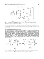
Figure 5 shows BER performance of N
t
x2 MIMO diversity system using the maximum ratio
combining (MRC) as a function of transmit signal to noise power ratio, where average gain
of channel is unity. Figure 6 also shows BER performance of 2xN
r
MIMO MRC diversity
system. In Figs. 5 and 6, the data stream is transmitted by the first eigenpath. Therefore, it
can be seen that both methods (LMS, SVD) achieve almost the same BER performance. This
result suggests that the eigenvector corresponding to the highest eigenvalue is correctly
detected as the first weight vector, i.e., the first eigenpath. It can be also qualitatively
explained that the highest eivenvalue is first found as the most dominant parameter
determining the error signal.
Figures 7 and 8 show BER performance of N
t
×2 and 2×N
r
E-MIMO, respectively. The number
of data streams is set to two, since the rank of channel matrix is two. Based on the BER
minimization criterion [1], the achievable BER is minimized by multiplying the transmit signal
by the inverse of the corresponding eigenvalue at the transmitter. In Figs. 7 and 8, we can see
that both methods (LMS and SVD) achieve almost the same BER performance.
Figures 9 and 10 show the MIMO channel capacity in case of two data streams. In this paper,

for simplicity, MIMO channel capacity is defined as the sum of each eigenpath channel
capacity which is calculated based on Shannon channel capacity in AWGN channel [3];
C = log
2
(1+SNR) [bit/s/Hz] (17)
MIMO Systems, Theory and Applications

272
The transmit power allocation for each eigenpath is determined based on the water-filling
theorem [3]. In Figs.9 and 10, it can be seen that the E-SDM system with the proposed
method achieves the same channel capacity as that of the ideal one (SVD).



Fig. 4. Measured eigenvalues



Fig. 5. Bit error rate performance (1 data stream, N
t
×2)
Iterative Optimization Algorithms to Determine Transmit and Receive Weights for MIMO Systems

273





Fig. 6. Bit error rate performance (1 data stream, 2×N

r
)





Fig. 7. Bit error rate performance (2 data stream, N
t
×2)
MIMO Systems, Theory and Applications

274





Fig. 8. Bit error rate performance (2 data stream, 2×N
r
)





Fig. 9. Channel capacity performance (N
t
×2)
Iterative Optimization Algorithms to Determine Transmit and Receive Weights for MIMO Systems

275


Fig. 10. Channel capacity performance (2×N
r
)
3. Iterative optimization of the transmitter weights under constraint of the
maximum transmit power for an antenna element in MIMO systems
3.1 System model
Figure 11 shows MU-MIMO system considered in this paper, where K antenna elements
and single antenna element are equipped at the Base Station (BS) and Mobile Station (MS),
respectively. Single antenna is assumed for each Mobile Station (MS). The number of users
in SDMA is N. The receive signal at receive antenna Y=[y
1
, ⋅ ⋅ ⋅ ,y
N
]
T
is expressed as

HH H
rt r
=+YWHWXWn (18)
where superscript
T
and superscript
H
denote transpose and Hermitian transpose,
respectively. H is N×K complex channel metrics, W

t
is N×K complex transmit weight
matrices, W
r
=diag(w
1
, ⋅ ⋅ ⋅, w
N
) is receive weight metrics, X=[x
1
, ⋅ ⋅ ⋅,x
N
]
T
is transmit signal,
and μ=[n
1
, ⋅ ⋅ ⋅,n
N
]
T
is noise signal. The average power of transmit signal is unity (i.e., E[x
i
2
]
=1), where E[ ] denotes ensemble average operation) and there is no correlation between
each user signal (i.e., E[x
i1
x
i2

] =0), the condition to keep the total average transmit power to
be less than or equal to P
th
is given as

2
11
NK
i
j
th
ij
wP
==
≤
∑∑
(19)
where
w
ij
denotes the transmit weight of antenna #j for user #i. Then, the condition to
constrain the average transmit power per each antenna to be less than or equal to p
th
is
given as
MIMO Systems, Theory and Applications

276

2

1
N
i
j
th
i
wp
=
≤
∑
j
∀
(1
≤
j
≤
K) (20)

Base Station
Maximum permissible transmit
power per antenna:
th
p
#1
#K
H
User #1
User #N
Base Station
Maximum permissible transmit

power per antenna:
th
p
Maximum permissible transmit
power per antenna:
th
p
#1
#K
H
User #1
User #N

Fig. 11. MU-MIMO Systems

・・・
・・・・
H
H
t
W
r
W
ˆ
Base Station
User #1
1
n
1
w

1
ˆ
n
N
n
ˆ
1
x
N
x
1
ˆ
y
N
y
ˆ
1
y
#1
#K
Virtual Channel
& Receiver
Root Nyquist
Filter
Modulated
Signal
Root Nyquist
Filter
Modulated
Signal

Root Nyquist
Filter
Root Nyquist
Filter
weight
control
Root Nyquist
Filter
User #N
N
n
N
w
N
y
Root Nyquist
Filter
・・・
・・・・
H
H
t
W
r
W
ˆ
Base Station
User #1
1
n

1
w
1
ˆ
n
N
n
ˆ
1
x
N
x
1
ˆ
y
N
y
ˆ
1
y
#1
#K
Virtual Channel
& Receiver
Root Nyquist
Filter
Modulated
Signal
Root Nyquist
Filter

Modulated
Signal
Root Nyquist
Filter
Root Nyquist
Filter
weight
control
Root Nyquist
Filter
User #N
N
n
N
w
N
y
Root Nyquist
Filter

Fig. 12. System configurations

Pilot
Data
symbolsN
p
symbolsN
d
Pilot
Data

symbolsN
p
symbolsN
d

Fig. 13. Frame format
3.2 Transmitter and receiver model
Figure 12 shows the system configuration of the transmitter and receiver in MU-MIMO
system considered in this paper, where the number of transmit antennas and the number of
receive antennas are K and 1, respectively. A virtual channel and virtual receiver are
equipped with the transmitter to estimate mean square error at the receiver side, where
Iterative Optimization Algorithms to Determine Transmit and Receive Weights for MIMO Systems

277
ˆ
r
W
=diag(
1
ˆ
w,
⋅ ⋅ ⋅ ,
ˆ
w
N
) and
ˆ
n =[
1
ˆ

n , . . . ,
ˆ
n
N
]
T
denote the virtual receive weight and the
virtual noise, respectively. We assume that the average power of additive white Gaussian
noise (AWGN) is known to the transmitter, i.e., we assume
2
i
ˆ
nE
⎡
⎤
⎣
⎦
=E[n
i
2
]. Then, the receive
signal at the virtual receiver
ˆ
Y
is given as

ˆ
ˆˆ
ˆ
HH H

rt r
=+YWHWXWn
(21)
The transmit weights are optimized by minimizing the error signal between transmit and
receive signals at the virtual receiver under constraints given as Eqs.(19) and (20). Figure 13
shows a frame format assumed in this paper, where each frame consists of N
p
pilot symbols
and N
d
data symbols. Pilot symbols are known and used for optimizing the receive weights
on the receiver side.
3.3 Weight optimization
a. Problem Formulation
The transmit weights are optimized by minimizing the mean square error between transmit
and receive signals at the virtual receiver under constraint given as Eqs. (19) and (20). From
Eq.(21), the error signal between transmit signal X and receive signal at the virtual receiver
ˆ
Y
is given as

ˆ
ˆˆ
ˆ
HH H
rt r
e =−=− −XYXWHWXWn (22)
where e=[e
1
, . . . ,e

N
]. From Eqs.(19) and (20), the problem to minimize the mean square error
under two constraints can be formulated as the following constrained minimizing problem;
Minimize
2
()Ee
⎡
⎤
⎢
⎥
⎣
⎦
W

Subject to
2
11
() 0
NK
ij th
ij
gwP
==
=
−≤
∑∑
W
(23)

2

1
() 0
N
jijth
i
hwp
=
=
−≤
∑
W j
∀

where
⋅
denotes vector norm. W
is N×(N+K) complex matrix defined as W=[W
t
,
ˆ
r
W
].
b.
A EIPF based Approach for Weight Optimization
By introducing the extended interior penalty function (EIPF) method into the problem
shown in Eq.(23), this problem can be transformed into the following non-constrained
minimizing problem [11];
Minimize
{}

2
() () ()Ee r
⎡⎤
+Φ +Ψ
⎢⎥
⎣⎦
W
WW
Subject to
2
1
()
2()
if ( )
()
if ( )
g
g
g
g
ε
ε
ε
ε
−
⎧
−
≤
⎪
Φ=

⎨
−
>
⎪
⎩
W
W
W
W
W

MIMO Systems, Theory and Applications

278

1
() ()
K
j
j
ψ
=
Ψ=
∑
W
W

2
1
j

()
2()
j
if ( )
()
if ( )
j
j
h
j
h
h
h
ε
ε
ε
ψ
ε
−
⎧
−
≤
⎪
=
⎨
⎪
−
>
⎩
W

W
W
W
W

Here, ε(<0) and r(>0) denote the design parameters for non-constrained problem. In Eq.(24),
()Φ
W
and ()Ψ
W
increase rapidly as approaches to the boundary. When g(W) = ε and
h
j
(W)=ε, the continuity of ()
Φ
W
and ()
Ψ
W
is guaranteed as well as derivatives of these
two functions. Thus, Eq. (24) can be minimized by using the Steepest Descent method; W is
updated as

{}
2
(1) () () ()()mmEer
μ
⎛⎞
⎡⎤
+= −∇ +Φ +Ψ

⎜⎟
⎢⎥
⎣⎦
⎝⎠
WWwW WW
(28)
where μ is a step size to adjust the updating speed.
∇
w denotes a gradient with respect to
W, which is defined as

11 1 1
1
ˆ
ˆ
K
NNK N
www
ww w
⎡
⎤
∂∂∂
⎢
⎥
∂∂∂
⎢
⎥
⎢
⎥
∇=

⎢
⎥
∂∂ ∂
⎢
⎥
⎢
⎥
∂∂ ∂
⎣
⎦
W
0
0
"
#%# %
"
(29)
where j denotes an imaginary unit and

{}{}
Re() Im()
ij
i
j
i
j
j
w
ww
∂∂ ∂

=+
∂
∂∂
, (30)

{}{}
ˆˆ ˆ
Re() Im()
ii i
j
ww w
∂∂ ∂
=+
∂∂ ∂
, (31)
When
W is updated as in Eq. (28) at every symbols, Eq. (28) can be reduced to

{}
2
(1) () () ()()mm r
μ
⎡
⎤
+= −∇ +Φ +Ψ
⎢
⎥
⎣
⎦
W

WW eW WW. (32)
3.4 Performance evaluation
Performance of MU-MIMO system using the considered algorithm is evaluated by
computer simulation. Simulation parameters are shown in Table 2. As a channel model, we
consider a set of 8 plane waves transmitted in random direction within the angle range of 12
degrees at the BS. Each of the plane waves has constant amplitude and takes the random
phase distributed from 0 to 2π. All users are randomly distributed with a uniform
distribution in a range of the coverage area of a BS. Channel states and distribution of users
Iterative Optimization Algorithms to Determine Transmit and Receive Weights for MIMO Systems

279
change independently at every frame. Transmit weights are determined with recursive
calculation given in Eq.(32). Receive weights are determined by observing the pilot symbols.
The upper limit of the average transmit power for an antenna element normalized by the
upper limit of the total transmit power is denoted as

th
th
p
P
γ
= , (33)
where

1
1
K
γ
≤
≤ (34)

In Eq.(34), γ=1 corresponds to the case without constraint of per-antenna transmit power.
The minimum value of γ
is 1/K which corresponds to, the strictest case where per-antenna
transmit power is limited within the minimum value. The maximum permissible power per
user (P
th
/N) to noise power ratio is defined as

max
2
[]
SNR
th
i
P/N
E|n|
= (35)
where E[n
i
2
] denotes the average noise power corresponding to the user #i.

Channel Model Flat uncorrelated quasistatic Rayeigh fading
Modulation Method QPSK
Number of Pilot Symbols (N
p
) 34 [symbols/frame]
Number of Data Symbols (N
d
) 460 [symbols/frame]

Average propagation loss 0 [dB] (Except for Figs.20 and 21)
Antenna element spacing 5.25λ
Table 2. Simulation Parameters
Figures 14(a) and (b) show complementary cumulative distribution function (CCDF) of
average transmit power of transmit signal measured at every frames with respect to antenna
#1. The number of transmit antennas is set to 4 and 8, respectively. The number of users is 2.
The maximum permissible transmit power is set to P
th
=1.0, and average noise power is set
to E [n
i
2
]=0.1. From these figures, we can see that transmit power of the signal at antenna #1
can be kept below p
th
.
Figures 15 and 16 show the received SINR as a function of γ, where SNR
max
is set to 10 dB.
Note that SINR is the same as SNR when the number of users is 1. In these figures, we can
see that the degradation in SINR at γ=1/K is about 0.5dB and 0.6
～1.0dB for K=4 and 8 as
compared with the case of γ =1. It is shown that SINR is slightly degraded when γ ≤ 0.4 and
γ ≤ 0.3 for K=4 and K=8, respectively. This is because the probability that transmit power of
the signal at a certain antenna element exceeds γ becomes low as γ increases. The received
SINR is degraded as the number of users increases, because the diversity effect is reduced
attributable to the decrease of a degree of freedom on the number of antennas.
MIMO Systems, Theory and Applications

280

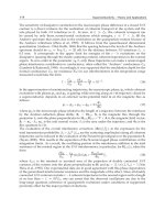
Figures 17 and 18 show BER performance as a function of SNR
max
, where the number of
users is set to 1∼3 for K=4 in Fig.17, and set to 3 for K=8 in Fig.18. In these figures, we can
see that, when the maximum per-antenna transmit power is limited to 1/K, BER
performances is degraded by about 0.7∼0.8 dB at BER=10
-2
as compared with case of γ=1.




(a) K=4, N=2



(b) K=8, N=2

Fig. 14. CCDF of average transmit power of the signal measured at every frames with
respect to antenna #1
Iterative Optimization Algorithms to Determine Transmit and Receive Weights for MIMO Systems

281

Fig. 15. SINR vs. γ (K=4, SNR
max
=10dB)








Fig. 16. SINR vs. γ (K=8, SNR
max
=10dB)
MIMO Systems, Theory and Applications

282






Fig. 17. Bit Error Rate Performance (K=4)

Fig. 18. Bit Error Rate Performance (K=8, N=3)
Iterative Optimization Algorithms to Determine Transmit and Receive Weights for MIMO Systems

283
4. Conclusion
We proposed optimization algorithms of transmit and receive weights for MIMO systems,
where the transmitter is equipped with a virtual MIMO channel and virtual receiver to
calculate the transmitter weight. First, we proposed an iterative optimization of transmit
and receive weights for E-SDM systems, where a least mean square algorithm is used to
determine the weight coefficients. The proposed method can be easily extended to the case
of E-SDM in MIMO system with arbitrary number of transmit and receive antennas. Second,
we proposed a weight optimization method of MIMO systems under constraints of the total
transmit power for all antenna elements and the maximum transmit power for an antenna
element. The performance of the proposed method is evaluated for QPSK signal in MU-
MIMO system with K antenna elements on the transmitter side and single antenna element
at the receive side. It is clarified that the degradation of received SINR attributable to
constraint of per antenna power is 0.5∼1.0 dB in case where the maximum transmit power
for an antenna element is limited to 1/K for the number of antenna of K=4 and 8. These
results mean that the proposed optimization algorithm enables to use a low cost power
amplifier at base stations in MIMO systems.
5. References
[1] T. Ohgane, T. Nishimura, & Y. Ogawa. Applications of Space Division Multiplexing and
Those Performance in a MIMO Channel, IEICE Transactions on Communications,
vol.E88-B, no.5, pp.1843-1851, May. 2005.
[2] G. Lebrun, J. Gao, & M. Faulkner. MIMO Transmission Over a Time-Varying Channel
Using SVD, IEEE Transactions on Wireless Communications, vol. 4, No.2, pp. 757 764,
March 2005.
[3] J. G. Proakis. Digital Communications, Fourth Edition, McGraw-Hill, 2001.
[4] S. Haykin. Adaptive Filter Theory, Fourth Edition, Prentice Hall, 2002.

[5] H. Yoshinaga, M.Taromaru, & Y.Akaiwa. Performance of Adaptive Array Antenna with
Widely Spaced Antenna Elements, Proceedings of the IEEE Vehicular Technology
Conference Fall'99, pp.72-76, Sept. 1999.
[6] T. Nishimura, Y. Takatori, T. Ohgane, Y. Ogawa, & K. Cho, Transmit Nullforming for a
MIMO/SDMA Downlink with Receive Antenna Selection, Proceedings of the IEEE
VTC Vehicular Technology Conference Fall’02, pp.190-194, Sept. 2002.
[7] Y. Kishiyama, T. Nishimura, T. Ohgane, Y. Ogawa, & Y. Doi. Weight Estimation for
Downlink Null Steering in a TDD/SDMA System, Proceedings of the IEEE VTC
Vehicular Technology Conference Spring'00, pp.346-350, May 2000.
[8] Y. Doi, Tadayuki Ito, J. Kitakado, T. Miyata, S. Nakao, T. Ohgane, & Y. Ogawa. The
SDMA/TDD Base Station for PHS Mobile Communication, Proceedings of the IEEE
Vehicular Technology Conference Spring'02, pp.1074-1078, May 2002.
[9] T. Nishimura, T. Ohgane, Y. Ogawa, Y. Doi, & J. Kitakado. Downlink Beamforming
Performance for an SDMA Terminal with Joint Detection, Proceedings of the IEEE
Vehicular Technology Conference Fall'01, pp.1538-1542, Oct. 2001.
[10] B. S. Krongold. Optimal MIMO-OFDM Loading with Power-Constrained Antennas,
Proceedings of the IEEE PIMRC'06, Sept. 2006.