Heat Transfer Engineering Applications Part 10 ppt

11
Mathematical Modelling of Dynamics of
Boiler Surfaces Heated Convectively
Wiesław Zima
Cracow University of Technology
Poland
1. Introduction
In order to increase the efficiency of electrical power production, steam parameters, namely
pressure and temperature, are increased. Changes in the superheated steam and feed water
temperatures in boiler operation are also caused by changes in the heat transfer conditions
on the combustion gases side. When the waterwalls of the furnace chamber undergo
slagging up, the combustion gases temperature at the furnace chamber outlet increases, and
the superheaters and economizers take more heat. In order to maintain the same
temperature of the superheated steam at the outlet, the flow of injected water must be
increased. Upon cleaning the superheater using ash blowers, the heat flux taken by the
superheater also increases, which in turn changes the coolant mass flow. Changes of the
superheated steam and feed water temperatures caused by switching off some burners or
coal pulverizers or by varying the net calorific value of the supplied coal may also be
significant. Precise modelling of superheater dynamics to improve the quality of control of
the superheated steam temperature is therefore essential. Designing the mathematical
model describing superheater dynamics is also very important from the point of view of
digital control of the superheated steam temperature. A crucial condition for its proper
control is setting up a precise numerical model of the superheater which, based on the
measured inlet and outlet steam temperature at the given stage, would provide fast and
accurate determination of the water mass flow to the injection attemperator. Such a
mathematical model fulfils the role of a process “observer”, significantly improving the
quality of process control (Zima, 2003, 2006). The transient processes of heat and flow
occurring in superheaters and economizers are complex and highly nonlinear. That
complexity is caused by the high values of temperature and pressure, the cross-parallel or
cross-counter-flow of the fluids, the large heat transfer surfaces (ranging from several
hundred to several thousand square metres), the necessity of taking into account the

increasing fouling of these surfaces on the combustion gases side, and the resulting change
in heat transfer conditions. The task is even more difficult when several heated surfaces are
located in parallel in one combustion gas duct, an arrangement which is applied quite often.
Nonlinearity results mainly from the dependency of the thermo-physical properties of the
working fluids and the separating walls on the pressure and temperature or on the
temperature only. Assumption of constancy of these properties reduces the problem to
steady state analysis. Diagnosis of heat flow processes in power engineering is generally

Heat Transfer – Engineering Applications

260
based on stabilized temperature conditions. This is due to the absence of mathematical
models that apply to big power units under transient thermal conditions (Krzyżanowski &
Głuch, 2004). The existing attempts to model steam superheaters and economizers are based
on greatly simplified one-dimensional models or models with lumped parameters
(Chakraborty & Chakraborty, 2002; Enns, 1962; Lu, 1999; Mohan et al., 2003). Shirakawa
presents a dynamic simulation tool that facilitates plant and control system design of
thermal power plants (Shirakawa, 2006). Object-oriented modelling techniques are used to
model individual plant components. Power plant components can also be modelled using a
modified neural network structure (Mohammadzaheri et al., 2009). In the paper by Bojić and
Dragićević a linear programming model has been developed to optimize the performance
and to find the optimal size of heating surfaces of a steam boiler (Bojić & Dragićević, 2006).
In this chapter a new mathematical method for modelling transient processes in
convectively heated surfaces of boilers is proposed. It considers the superheater or
economizer model as one with distributed parameters. The method makes it possible to
model transient heat transfer processes even in the case of fluids differing considerably in
their thermal inertias.
2. Description of the proposed model
Real superheaters and economizers are three-dimensional objects. The basic assumptions of
the proposed model refer to the parameters of the working fluids. It was assumed that there

are no changes in combustion gases flow and temperature in the arbitrary cross-section of
the given superheater or economizer stage (Dechamps, 1995). The same applies to steam and
feed water. When the real heat exchanger is operating in cross-counter-flow or cross-
parallel-flow and has more than four tube rows, its one-dimensional model (double pipe
heat exchanger), represented by Fig. 1, can be based on counter-flow or parallel-flow only
(Hausen, 1976). In the proposed model, which has distributed parameters, the computations
are carried out in the direction of the heated fluid flow in one tube. The tube is equal in size
to those installed in the existing object and is placed, in the calculation model, centrally in a
larger externally insulated tube of assumed zero wall thickness (Fig. 1). The cross-section A
cg

of the combustion gases flow results, in the computation model, from dividing the total free
cross-section of combustion gases flow by the number of tubes. The mass flows of the
working fluids are also related to a single tube.
A precise mathematical model of a superheater, based on solving equations describing the
laws of mass, momentum, and energy conservation, is presented in (Zima, 2001, 2003, 2004,
2006). The model makes it possible to determine the spatio-temporal distributions of the
mass flow, pressure, and enthalpy of steam in the on-line mode. This chapter presents a
model based solely on the energy equation, omitting the mass and momentum conservation
equations. Such a model results in fewer final equations and a simpler form. Their solution
is thereby reached faster. The short time taken by the computations (within a few seconds) is
very important from the perspective of digital temperature control of superheated steam. In
the papers by Zima that control method was presented for the first time (Zima, 2003, 2004,
2006). In this case the mathematical model fulfils the role of a process “observer”,
significantly improving the quality of process control. The omission of the mass and
momentum balance equations does not generate errors in the computations and does not
constitute a limitation of the method. The history of superheated steam mass flow is not a

Mathematical Modelling of Dynamics of Boiler Surfaces Heated Convectively

261
rapidly changing one. Also taking into consideration the low density of the steam, it is
possible to neglect the variation of steam mass existing in the superheater. Feed water mass
flow also does not change rapidly. Moreover the water is an incompressible medium. The
results of the proposed method are very similar to results obtained using equations
describing the laws of mass, momentum, and energy conservation (Zima, 2001, 2004).
The suggested in this chapter 1D model is proposed for modelling the operation of
superheaters and economizers considering time-dependent boundary conditions. It is based
on the implicit finite-difference method in an iterative scheme (Zima, 2007).


Fig. 1. Analysed control volume of double-pipe heat exchanger
Every equation presented in this section is based on the geometry shown in Fig. 1 and refers
to one tube of the heated fluid. The Cartesian coordinate system is used.
The proposed model shows the same transient behaviour as the existing superheater or
economizer if:
a. the steam or feed water tube has the same inside and outside diameter, the same length,
and the same mass as the real one
b. all the thermo-physical properties of the fluids and the material of the separating walls
are computed in real time
c. the time-spatial distributions of heat transfer coefficients are computed in the on-line
mode, considering the actual tube pitches and cross-flow of the combustion gases
d. the appropriate free cross-sectional area for the combustion gases flow is assumed in
the model:



22
1
,

4
in o
cg t
cg
dd
A
A
n


 (1)
e.
mass flow of the heated fluid is given by:

t
m
m
n



(2)

Heat Transfer – Engineering Applications

262
f. mass flow of the combustion gases is given by:

,c
g

t
cg
m
m
n



. (3)
In the above equations:
A
cg, t
– total free cross-section of combustion gases flow, m
2
,
,c
g
t
m

– total combustion gases mass flow, kg/s,
t
m

– total heated fluid mass flow, kg/s,
n – number of tubes.
The temperature

of the separating wall is determined from the equation of transient heat
conduction:

  
1
ww w
crk
trr r


  











, (4)
where:
c
w
– specific heat of the tube wall material, J/(kg K),
k
w
– thermal conductivity of the tube wall material, W/(mK),

w

– density of the tube wall material, kg/m
3
.
In order to obtain greater accuracy of the results, the wall is divided into two control
volumes. This division makes it possible to determine the temperature on both surfaces of
the separating wall, namely

cg
at the combustion gases side and

h
at the heated medium
side (Fig. 2).


Fig. 2. Tube wall divided into two control volumes
After some transformations, the following formulae are obtained from Equation 4:

 


 
22
2
min
min
h
wh wh w w
rr rr
rr

crkrk
tr r


  








 

, (5)




 
22
2
om
om
cg
wcg wcg w w
rr rr
rr
crkrk

tr r


  








 

. (6)
Taking into consideration the boundary conditions:

Mathematical Modelling of Dynamics of Boiler Surfaces Heated Convectively

263




in
in
wrrh
rr
khThT
r


 




 

, (7)



m
c
g
h
wwm
oin
rr
kk
rrr










, (8)





o
o
wc
g
c
g
c
g
c
g
c
g
rr
rr
khThT
r









, (9)
where:
h and h
cg
– heat transfer coefficients at the sides of heated fluid and combustion gases,
respectively, W/(m
2
K),
the following ordinary differential equations are obtained:



d
d
h
c
g
hh
BCT
t




, (10)


d
d
cg

c
g
c
g
hc
g
DT E
t



. (11)
In the above equations:


   
,,, ,
22
cg h
mw m
in o in
mm
hw h w h w hw h w h
dk
dd hd
Bd C
Ac g Ac





 




cg o
c
g
wc
g
wc
g
hd
D
Ac



 ,




22
,,
4
min
mw m
h

cg w cg w cg w
dd
dk
EA
Ac g




 and


22
4
om
cg
dd
A


 .
The transient temperatures of the combustion gases and heated fluid are evaluated
iteratively, using relations derived from the equations of energy balance. In these equations,
the change in time of the total energy in the control volume, the flux of energy entering and
exiting the control volume, and the heat flux transferred to it through its surface are taken
into consideration.
The energy balance equations take the following forms (Fig. 1):
-
combustion gases

  
cg
c
g
c
g
c
g
c
g
c
g
c
g
c
g
c
g
c
g
c
g
oc
g
c
g
zz z
T
zA c T T m i m i h d z T
t







 

, (12)
-
feed water or steam



,,
in h
zzz
T
zAc T p T p m i m i h d z T
t






, (13)
where:
i – specific enthalpy, J/kg,

Heat Transfer – Engineering Applications

264
p – pressure, Pa,
22
1
4
in o
cg
dd
A



 , and
2
4
in
d
A

 .
After rearranging and assuming that Δt → 0 and Δz → 0, the following equations are
obtained from (12) and (13), respectively:


cg cg
c
g
c

g
TT
FGT
tz


  

, (14)


h
TT
HJT
tz





. (15)
In the above equations:
  

,,
,
cg cg o
cg cg cg cg cg cg cg cg
mhd
m

FG H
AT
p
AT AcT T



 


and

,,
in
hd
J
Ac T p T p


 .
The sign “+” in Equations (12) and (14) refers to counter-flow, and the sign “ – ” to parallel-
flow. The implicit finite-difference method is proposed to solve the system of Equations (10)
to (11) and (14) to (15). The time derivatives are replaced by a forward difference scheme,
whereas the dimensional derivatives are replaced by the backward difference scheme in the
case of parallel-flow and the forward difference scheme in the case of counter-flow.
After some transformations the following formulae are obtained:

,, ,
1
tt t tt tt

h
j
h
jj
c
gj
CB
T
Kt K K
 




, j = 1, , M; (16)

,,,,
1
tt t tt tt
c
gj
c
gj
c
gj
h
j
DE
T
Lt L L

 




, j = 1, , M; (17)

,,,1,
1
tt t tt tt
c
gj
c
gj
c
gj
c
gj
FG
TTT
Pt Pz P




 


, (18)

1,
1
tt t tt tt
jjj
h
j
HJ
TTT
Qt Qz Q




 

, j = 2, , M; (19)
where:
M – number of cross-sections,
11 1
,,
F
KBCLDEP G
tt tz
  
 
, and
1 H
QJ
tz




.
In Equation (18), j = 2, . . . , M for parallel-flow (sign “−”) and j = 1, . . . , M −1 for counter-
flow (sign “+”).
Considering the small temperature drop on the thickness of the wall (≈ 3–4 K), Equation (4)
can also be solved assuming only one control volume. The result will be a formula
determining only the mean temperature

of a wall (Fig. 2).

Mathematical Modelling of Dynamics of Boiler Surfaces Heated Convectively

265
In this case, after some transformations, Equation (4) takes the following form:

 


 
22
2
oin
oin
ww w w
rr rr
rr
crkrk
tr r
 

   


 



 

. (20)
Taking into consideration the boundary conditions described by Equations (7) and (9), the
following ordinary differential equation is obtained:



d
d
cg
UT VT
t




 
. (21)
Replacing the time derivative by the forward difference scheme, after rearranging we
obtain:

,

1
tt t tt tt
jjcgjj
UV
TT
Wt W W



 

, (22)
where:
   
,,
2
cg o
in o in
m
wwwm wwwm
hd
hd d d
UVd
cgdcgd
   

  and
1
WUV
t




.
The suggested method is also suitable for modelling the dynamics of several surfaces heated
convectively, often placed in parallel in a single gas pass of the boiler.
As an example of these surfaces it was assumed that the feed water heater and superheater
are located in parallel in such a gas pass (Fig. 3). Additionally, the flow of combustion gases
is in parallel-flow with feed water and simultaneously in counter-flow to steam.
The equation of transient heat conduction (Equation 4) takes the following forms (the walls
of steam and feed water pipes are divided into two control volumes):
-
wall of steam pipe




 
22
1
11
11 1 1
2
min
min
s
wsws w w
rr rr
rr
crkrk

tr r


  








 

, (23)




 
22
1
11
11 1 1
2
om
om
cg
wcgwcg w w
rr rr

rr
crkrk
tr r


  








 

, (24)
-
wall of economizer pipe




 
22
22
22
2
22
22 2 2

2
min
min
fw
wfwwfw w w
rr rr
rr
crkrk
tr r


  







 

, (25)




 
22
22
22

2
22
22 2 2
2
om
om
cg
wcgwcg w w
rr rr
rr
crkrk
tr r


  







 

. (26)

Heat Transfer – Engineering Applications

266

Fig. 3. Analysed control volume of several surfaces heated convectively, placed in parallel in
a single gas pass
Substituting the appropriate boundary conditions, the following differential equations are
obtained after some transformations:



1
11 1 1 1
d
d
s
c
g
sss
BCT
t




, (27)


1
11111
d
d
cg

c
g
c
g
sc
g
DT E
t


, (28)


2
12 2 1 2
d
d
fw
c
gf
w
f
w
f
w
FGT
t

 
, (29)

 
2
12122
d
d
cg
c
g
c
gf
wc
g
HT J
t


. (30)

Mathematical Modelling of Dynamics of Boiler Surfaces Heated Convectively

267
In the above equations:


 

1
111
11 1 11 1

11 1
,, ,
cg o
wm m
sin
sw s w s w sw s w s
cg w cg w cg
hd
kd
hd
BCD
Ac g Ac
Ac



 







 
2
122
11 1
11 1 2 2 2 2 2 2
,,,

fw in
wm m wm m
cg w cg w cg w fw w fw w fw w fw w fw w fw
hd
kd kd
EF G
Ac g A c g A c

 
    
 




211
22
11 1
22 2 22 2
,,,
2
c
g
osc
g
wm m
m
cg w cg w cg cg w cg w cg w
hd
kd

HJ
Ac Ac g



 

 




22 22
22
22
2211
,, , , ,
22 2 4 4
min om
fw cg
in o in o
mmms cg
dd dd
dd d d
dd A A










22
22
2
,
4
min
fw
dd
A


 and


22
22
2
4
om
cg
dd
A


 .
The energy balance equations take the following forms (Fig. 3):

-
combustion gases

 
 
122
cg
cg cg cg cg cg cg cg cg cg
zzz
cg o cg cg cg o cg cg
T
zA c T T m i m i
t
hdz T hdz T

  





 

(31)
-
steam



1

,,
s
ss s s s s s ss ss s in s s
zz z
T
zA c T p T p m i m i h d z T
t






, (32)
-
feed water

 
22
,,
fw
f
w
f
w
f
w
f
w
f

w
f
w
f
w
f
w
f
w
f
w
f
w
f
win
f
w
f
w
zzz
T
zA c T p T p m i m i h d z T
t






, (33)

where:
222 2
12
,
444 4
in o o in
cg s
ddd d
AA
 

 



, and
2
2
.
4
in
fw
d
A


After rearranging and assuming that t0 and z0, the following formulae were obtained
(from Equations (31)–(33), respectively):



11 12 1
c
g
c
g
cg cg cg cg
TT
KTLTP
tz





, (34)

Heat Transfer – Engineering Applications

268


11 1
ss
ss
TT
QTR
tz







, (35)


12 1
f
w
f
w
fw fw
TT
STU
tz





, (36)
where:
    

2
1111
,,,,
,
cg o cg o cg
s

ss s s
cg cg cg cg cg cg cg cg cg cg cg cg cg
hd hd m
m
KLPR
ATp
Ac T T Ac T T A T









2
11
,,
,,
,,
fw in
sin
ss s s s s s
fw fw fw fw fw fw fw
hd
hd
QS
Ac T p T p
AcTp Tp





 and

1
.
,
fw
fw fw fw fw
m
U
ATp




To solve the system of Equations (27) to (30) and (34) to (36) the implicit finite-difference
method was used. After some transformations the following dependencies were obtained:

11
1, 1, 1 , ,
1
tt t tt tt
s
j
s
j
c

gj
s
j
BC
T
Vt V V





, j = 1, , M; (37)

11
1, 1, , 1,
111
1
tt t tt tt
c
gj
c
gj
c
gj
s
j
DE
T
Vt V V
 





, j = 1, , M; (38)

11
2, 2, 2, ,
1
tt t tt tt
f
w
jf
w
j
c
gj f
w
j
FG
T
Wt W W





, j = 1, , M; (39)

11

2, 2, , 2 ,
111
1
tt t tt tt
c
gj
c
gj
c
gj f
w
j
HJ
T
Wt W W
 




, j = 1, , M; (40)

11 1
,,1,2,,1
1111
1
tt t tt tt tt
c
gj
c

gj
c
gj
c
gj
c
gj
KL P
TT T
Xt X X Xz

   



, j = 2, , M; (41)

11
,,1,,1
111
1
tt t tt tt
s
j
s
j
s
j
s
j

QR
TT T
Yt Y Yz






, j = 1, , M-1; (42)

11
,,2,,1
111
1
tt t tt tt
f
w
jf
w
jf
w
jf
w
j
SU
TT T
Zt Z Zz

  




, j = 2, , M. (43)
In the above equations:
111 11 11 1 11
11 1 1
,,, ,
VBCV DEWFGW HJ
tt t t
   
  

11
11111
11
,
PR
XKL YQ
tztz
 


, and
1
11
1 U
ZS
tz




.

Mathematical Modelling of Dynamics of Boiler Surfaces Heated Convectively

269
In view of the iterative character of the suggested method, the computations should satisfy
the following condition:

,( 1) ,( )
,( 1)
tt tt
jk jk
tt
jk
YY
Y

 





(44)
where
Y is the currently evaluated temperature in node j; ϑ is the assumed tolerance of
iteration; and
k = 1, 2, . . . is the next iteration counter after a single time step.

Additionally, the following condition – the Courant–Friedrichs–Lewy stability condition
over the time step – should be satisfied (Gerald, 1994):

1,
z
t
w



, (45)
where:
wt
z




is the Courant number.
When satisfying this condition, the numerical solution is reached with a speed
z/t, which
is greater than the physical speed
w.
3. Computational verification
The efficiency of the proposed method is verified in this section by the comparison of the
results obtained using the method and from the corresponding analytical solutions. Exact
solutions available in the literature for transient states are developed only for the simplest
cases. In this section a step function change of the fluid temperature at the tube inlet and a
step function heating on the outer surface of the tube are analysed.
3.1 Analytical solutions for transient states

The available analytical dependencies allow the following to be determined (Serov &
Korolkov, 1981):
-
the time-spatial temperature distribution of the tube wall, insulated on the outer
surface, as the tube’s response to the temperature step function of the fluid at the tube
inlet,
-
the time-spatial temperature distribution of the fluid in the case of a heat flux step
function on the outer surface of the tube.
3.1.1 Temperature step function of the fluid at the tube inlet
The analysed step function is assumed as follows (Fig. 4):


0for 0,
1for 0.
t
Tt
t






(46)
For this step function, the dimensionless dependency determining the increase of the tube
wall temperature takes the following form:

10
VV

T





, (47)

Heat Transfer – Engineering Applications

270


Fig. 4. Temperature step function of the fluid at the tube inlet
where:




1
,Ve U




 , (48)






00
2Ve I




 . (49)
The


,U


function is described by the following dependency:


00
,
!!
nk
n
nk
U
nk








, (50)
and the Bessel function:




0
2
0
2
!
k
k
I
k







. (51)
Values

and

present in Formulae (48)–(51) are the dimensionless variables of length and

time respectively, expressed by the following dependencies:



22
;,
TP
tt z
z
FD



(52)
where:


2TP
z
tzB
w



. (53)
Coefficients
B
2
, D
2

, and F
2
are described in Section 3.2.
3.1.2 Heat flux step function on the outer surface of the tube
A dimensionless time-spatial function describing the increase of the fluid temperature ΔT,
caused by the heat flux step function Δ
q on the outer surface of the tube, is expressed as:

Mathematical Modelling of Dynamics of Boiler Surfaces Heated Convectively

271

102
2
2
1
1
1
Tt
V
c
Dc
Eq
c



 




. (54)
In the above formula:
c = – D
2
/B
2
;

q and coefficient E
2
are described in Section 3.2.
Functions

0
and V
2
are described by the following dependencies:


2
1
0100
1
t
c
D
eVV



   , (55)



 
201
,2 2Ve U I I


      



  




, (56)
where:



 
21
2
1
0
2
!1!

k
k
I
kk








. (57)
Function
V
00
present in Formula (55) is expressed as:


00
,Ve U c
c









. (58)
The analytical dependencies (47) and (54) presented above allow the time-spatial
temperature increases, Δ

for the tube wall and ΔT for the fluid, to be determined for any
selected cross-section. The results are obtained beginning from time
t
TP
(z) = z/w, that is,
from the moment this cross-section is reached by the fluid flowing with velocity
w. For
example, if the flow velocity equals 1m/s, then the analytical solutions allow the
temperature changes for the cross-section located 10 m away from the inlet of the tube to be
determined only after 10 s.
3.2 Application of the proposed method for the purpose of verification
In order to compare the results obtained using the suggested method with the results of
analytical solutions for transient states, the appropriate dependencies are derived for the
control volume shown in Fig. 5.
Assuming one control volume of the tube wall, Equation (4) takes the form of Equation (20).
Taking into consideration the boundary conditions:


o
w
rr
kq
r







, (59)
and





in
in
w
rr
rr
khThT
r

 




 

, (60)

Heat Transfer – Engineering Applications

272

the following differential equation is obtained:

22
d
d
DTEq
t



 
. (61)
In the above equation:




2
wwmw
in
cdg
D
hd
 
 ,
2
1
in
E
hd


 , and
2
oin
m
dd
d


.
Moreover, the heat flux step function is described as:

qqs


, (62)
where:
q – heat flux, W/m
2
,
s – actual tube pitch, m.


Fig. 5. Analysed control volume
On the side of the working fluid the energy balance equation takes the form of Equation
(13), in which the mean wall temperature

is used instead of

h

:



,,
in
zzz
T
zAc T p T p m i m i h d z T
t




 


. (63)
Assuming that
t  0 and z  0, the following equation is obtained:

22
TT
BTF
tz







, (64)
where:




2
,,
in
Ac T p T p
B
hd



,


2
,
in
mc T p
F
hd



and
2

4
in
d
A

 .

Mathematical Modelling of Dynamics of Boiler Surfaces Heated Convectively

273
To solve the system of Equations (61) and (64), the implicit finite difference method was
used, and after transformations we obtain:


2
2
22
tt t tt tt
jjjj
Dt
TEq
Dt tD

  



 




  


, j = 1, , M (65)

22
1
22
1
tt t tt
jjj
tt
j
BF
TT
tz
T
BF
tz











, j = 2, , M. (66)
3.3 Results and discussion
As an illustration of the accuracy and effectiveness of the suggested method the following
numerical analyses are carried out:
-
for the tube with the temperature step function of the fluid at the tube inlet,
-
for the tube with the heat flux step function on the outer surface.
The results obtained are compared afterwards with the results of analytical solutions. In
both cases the working fluid is assumed to be water. The heat transfer coefficient is taken as
constant and equals
h = 1000 W/(m
2
K). Because the exact solutions do not allow the
temperature dependent thermo-physical properties to be considered, the following constant
water properties were assumed for the computations:

= 988 kg/m
3
and c = 4199 J/(kgK).
For both cases it was also assumed that the tube is
L = 131 m long, its external diameter
equals
d
o
= 0.038 m, the wall thickness is g
w
= 0.0032 m, and the tube is made of K10 steel of
the following properties:


w
= 7850 kg/m
3
and c
w
= 470 J/(kgK). Satisfying the Courant
condition (45), the following were taken for the computations:
z = 0.5 m, t = 0.1 s and
w = 1 m/s ( m

= 0.775 kg/s).


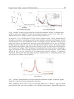
Fig. 6. Dimensionless histories of tube wall temperature increase

Heat Transfer – Engineering Applications

274
In the first numerical analysis it was assumed that water of initial temperature T = 20
o
C
flows through the tube. Also, the tube wall for the initial time
t = 0 has the same initial
temperature. Beginning from the next time step, the fluid of temperature
T = 100
o
C appears
at the inlet. The temperature step function is thus
T = 80 K. The results of the computations
are presented in Fig. 6. The presented dimensionless coordinates

 = 0, 2, and 4 correspond
with the dimensional coordinates
z = 0, 65.5 m, and 131 m respectively. An analysis of the
comparison shows satisfactory convergence of the exact solution results with the results
obtained using the presented method.
In the second case it was assumed that the working fluid and the tube at time
t = 0 take the
initial temperature
T =

= 70
o
C. Starting from the next time step, the heat flux step function
(

q = qs) appears on the outer surface of the tube. The assumed heat load is the heat flux
q = 10
5
W/m
2
and the tube pitch s = 0.041 m. The selected results of the numerical analysis,
comprising a comparison of the dimensionless histories of the fluid temperature increase for
the same cross-sections as in the first case, are shown in Fig. 7.


Fig. 7. Histories of dimensionless fluid temperature increase
These histories begin from the time instants

= 5.04 (t = 65.5 s), and


= 10.08 (t = 131 s),
respectively, that is, from the moment the analysed cross-sections were reached by the fluid
flowing with the velocity
w = 1 m/s. A satisfactory convergence of the results of the
analytical solution with the results obtained using the suggested method was achieved.
4. Experimental verification
This section describes the experimental verification of the proposed method for modelling
transient processes which occur in power boilers surfaces heated convectively. Transient
state operation of the platen superheater during the start-up of an OP-210 boiler was
analysed. The boiler capacity is 210
10
3
kg/h of live steam with 9.8 MPa pressure and
5
10
540



o
C temperature. The platen superheater (Figs. 8 and 13) consists of 14 vertical screens

Mathematical Modelling of Dynamics of Boiler Surfaces Heated Convectively

275
installed with 520 mm transversal pitch. Each screen consists of 13 tubes ( 32 × 5 mm)
placed with 36 mm longitudinal pitch. The heated surface of the superheater is 406 m
2

(

n = 182 tubes) and the total free cross-section of the combustion gases flow is A
cg,t
= 64.5 m
2
.
The tubes, each
L = 26.3 m long, are made of 12H1MF steel and placed in 52 rows. As the
analysed platen superheater is operating in cross-parallel-flow, a parallel-flow arrangement
was assumed for numerical modelling.
The time-spatial heat transfer coefficients for steam and combustion gases were computed in
the on-line mode using dependencies published in (Kuznetsov et al., 1973). Moreover, based
on the data given by (Meyer et al., 1993; Kuznetsov et al., 1973; Wegst, 2000) appropriate
functions were created. These functions allow the thermo-physical properties of the steam,
combustion gases and the material of the tube wall to be computed in real time.
The platen superheater tube was divided into
M = 16 cross-sections (z = 1.75 m). The time
step of computations was taken at
t = 0.1 s.


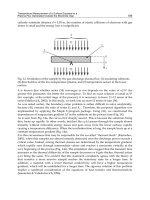
Fig. 8. Location of platen superheater
In order to model the dynamics of the platen superheater it is necessary to know the
transient values of temperature, pressure, and total mass flow of steam and combustion
gases at the superheater inlet. On the steam side, these values were known from
measurements and are shown in Figs. 9 and 11 (curve b), whereas at the combustion gases
side they were computed (Fig. 10). To calculate the pressure drop of the steam (in the
direction of the steam flow), the Darcy-Weisbach equation was used.

Heat Transfer – Engineering Applications

276
The selection of a platen superheater for verification was not accidental. It is, namely,
located in the combustion gas bridge, just behind the furnace chamber (Fig. 8). The
computed values of combustion gases temperature and mass flow at the furnace chamber
outlet therefore constituted the input data for modelling the platen superheater operation.
In order to compute these transient values, the fuel mass flow should be determined first.
To find it, a method based on the known characteristics of the coal dust feeder in function
of its number of revolutions was used (Cwynar, 1981). The total mass flow of combustion
gases at the furnace chamber outlet was computed using stoichiometric combustion
equations and the known mass flow of combustion coal. The combustion gases
temperature at the furnace chamber outlet was determined by solving the equations of
energy and heat transfer for the boiler furnace chamber using the CKTI method
(Kuznetsov et al., 1973). The computed values of combustion gases temperature and mass
flow are shown in Fig. 10.
The measurements carried out on the real object were disturbed by errors resulting from the
degree of inaccuracy of the measuring sensors and converters.
These errors, related to the maximum measuring ranges, were as follows:
a.  3.3
o
C in the superheated steam temperature readings (measuring range: 0–600
o
C;
level of sensor inaccuracy: 0.25; level of converter inaccuracy: 0.3),
b.
 9610
3
Pa in the superheated steam pressure readings (measuring range: 0–16 MPa;
level of sensor inaccuracy: 0.6),
c.
 0.799 kg/s in the mass flow of superheated steam (measuring range: 0–69.44 kg/s;

level of measuring orifice inaccuracy: 1; level of converter inaccuracy: 0.15).




Fig. 9. Histories of the measured steam pressure and total mass flow at the platen
superheater inlet

Mathematical Modelling of Dynamics of Boiler Surfaces Heated Convectively

277



Fig. 10. Histories of the computed combustion gases temperature and total mass flow at the
platen superheater inlet (at the furnace chamber outlet)



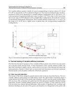
Fig. 11. Comparison of the measured and computed steam temperatures at the superheater
outlet (a) and history of the measured steam temperature at the superheater inlet (b)

Heat Transfer – Engineering Applications

278

Fig. 12. History of the computed combustion gases temperature at the superheater outlet
When comparing the results of steam temperature measurement at the platen superheater
outlet with the results of numerical computation, fully satisfactory convergence is found
(Fig. 11 – curve a). The divergences visible in Fig. 11 (curve a), in the range of 0 to about 30
min, result from the assumption in the calculation model that the initial temperature of the
analysed steam superheating system at time
t = 0 is equal to the measured steam
temperature at the superheater inlet, that is,
T = T
cg
=

h
=

cg
= 359
o
C.
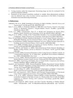
The computed combustion gases temperature at the platen superheater outlet (Fig. 12) can
be used for modelling the dynamics of steam superheaters located after it (Fig. 13). The two
stages, KPP-2 and KPP-3, of the superheater are installed parallel to each other in one gas

pass. The superheater KPP-2 operates in counter-flow, and KPP-3 operates in parallel-flow
to combustion gases. A comparison of the measured and computed steam temperature
histories at the KPP-3 outlet is presented in the paper (Zima, 2003).

Mathematical Modelling of Dynamics of Boiler Surfaces Heated Convectively

279





Fig. 13. Location of the analysed platen superheater and three stages of convective steam
superheater (KPP-1, KPP-2, and KPP-3)

Heat Transfer – Engineering Applications

280
The selected results of modelling the dynamics of the economizer installed in the convective
duct of the OP-210 boiler are presented in the paper (Zima, 2007). In the computations the
fins were considered on the combustion gases side, and the heat transfer coefficient was
calculated according to (Taler & Duda, 2006). The measured history of feed water
temperature at the economizer outlet was compared with the computational results and
satisfactory agreement was achieved.
5. Conclusions
The chapter presents a method for modelling the dynamics of boiler surfaces heated
convectively, namely steam superheaters and economizers. The proposed method
comprises solving the energy equations and considers the superheater or economizer model
as one with distributed parameters. The proposed model is one-dimensional and is suitable
for pendant superheaters and economizers. In this model, the boundary conditions can be

time-dependent. The computations are carried out in the direction of the heated fluid flow
in one tube. The time-spatial temperature history of the separating wall is determined from
the equation of transient heat conduction. As the time-spatial heat transfer coefficients at the
working fluids sides are computed in the on-line mode considering the actual tube pitches
and cross-flow of combustion gases, the physics of the phenomena occurring in the
superheaters and economizers does not change. All the thermo-physical properties of the
fluids and the material of the separating walls are also computed in real time. In order to
prove the accuracy and effectiveness of the proposed method, computational and
experimental verifications were carried out. The analysis of the presented comparisons
demonstrates fully satisfactory convergence of the results obtained using the suggested
method with the results of analytical solutions and with measured temperature history.
When analysing the presented comparisons it should be considered that many parameters
affect the final result of the operation of the surfaces heated convectively (e.g. ones resulting
from gradual fouling of these surfaces). Not all these parameters can be fully taken into
consideration in the calculation algorithm.
6. References
Bojić, M. & Dragićević, S. (2006). Optimization of steam boiler design. Proceedings of the
Institution of Mechanical Engineers, Part A: Journal of Power and Energy
, Vol. 220, No. 6
(September 2006), pp. 629–634, ISSN 0957-6509
Chakraborty, N. & Chakraborty, S. (2002). A generalized object-oriented computational
method for simulation of power and process cycles.
Proceedings of the Institution of
Mechanical Engineers, Part A: Journal of Power and Energy
, Vol. 216, No. 2 (April
2002), pp. 155–159, ISSN 0957-6509
Cwynar, L. (1981).
Start-up of Power Boilers (in Polish), Scientific and Technical Publishing
Company, ISBN 83-204-0416-9, Warsaw
Dechamps, P.J. (1995). Modelling the transient behaviour of heat recovery steam generators.

Proceedings of the Institution of Mechanical Engineers, Part A: Journal of Power and
Energy
, Vol. 209, No. A4 (January 1995), pp. 265–273, ISSN 0957-6509

Mathematical Modelling of Dynamics of Boiler Surfaces Heated Convectively

281
Enns, M. (1962). Comparison of dynamic models of a superheater. ASME Transactions –
Journal of Heat Transfer
, Vol. 84, No. 4, pp. 375–385
Gerald, C.F. & Wheatley, P.O. (1994).
Applied numerical analysis, Addison-Wesley Publishing
Company, ISBN 0-201-56553-6, New York
Hausen, H. (1976).
Wärmeübertragung im Gegenstrom, Gleichstrom und Kreuzstrom (2nd ed.),
Springer Verlag, ISBN 3540075526, Berlin
Krzyżanowski, J. & Głuch, J. (2004).
Heat-Flow Diagnostics of Energetic Objects (in Polish),
Polish Academy of Sciences, ISBN 83-88237-65-9, Gdansk
Kuznetsov, N.V.; Mitor, V.V.; Dubovskij, I.E. & Karasina, E.S. (1973).
Standard Methods of
Thermal Design for Power Boilers
(in Russian), Central Boiler and Turbine Institute,
Energija, UDK 621.181.001.24:536.7, Moscow
Lu, S. (1999). Dynamic modelling and simulation of power plant systems.
Proceedings of the
Institution of Mechanical Engineers, Part A: Journal of Power and Energy
, Vol. 213, No. 1
(February 1999), pp. 7–22, ISSN 0957-6509
Meyer, C. A. et al. (1993).

ASME Steam Tables, American Society of Mechanical Engineers,
ISBN 0791806324, New York
Mohammadzaheri, M.; Chen, L.; Ghaffari, A. & Willison, J. (2009). A combination of linear
and nonlinear activation functions in neural networks for modeling a de-
superheater.
Simulation Modelling Practice & Theory, Vol. 17, No. 2 (February 2009),
pp. 398–407, ISSN 1569190X
Mohan, M.; Gandhi, O.P. & Agrawal, V.P. (2003). Systems modelling of a coal-based steam
power plant.
Proceedings of the Institution of Mechanical Engineers, Part A: Journal of
Power and Energy
, Vol. 217, No. 3 (June 2003), pp. 259–277, ISSN 0957-6509
Serov, E.P. & Korolkov, B.P. (1981).
Dynamics of Steam Generators (in Russian), Energoizdat,
UDK 621.181.016.7, Moscow
Shirakawa, M. (2006). Development of a thermal power plant simulation tool based on
object orientation.
Proceedings of the Institution of Mechanical Engineers, Part A:
Journal of Power and Energy
, Vol. 220, No. 6 (September 2006), pp. 569–579, ISSN
0957-6509
Taler, J. & Duda, P. (2006).
Solving Direct and Inverse Heat Conduction Problems, Springer,
ISBN 978-3-540-33470-5, Berlin
Wegst, C.W. (2000).
Key to Steel, Verlag Stahlschlüssel Wegst GmbH, ISBN 3922599176,
Marbach
Zima, W. (2001). Numerical modeling of dynamics of steam superheaters.
Energy, Vol. 26,
No. 12, (December 2001), pp. 1175–1184, ISSN 0360-5442

Zima, W. (2003). Mathematical model of transient processes in steam superheaters.
Forschung im Ingenieurwesen, Vol. 68, No. 1 (July 2003), pp. 51–59, ISSN 0015-7899
Zima, W. (2004).
Simulation of transient processes in boiler steam superheaters (in Polish),
Monograph 311, Publishing House of Cracow University of Technology, ISSN 0860-
097X, Cracow
Zima, W. (2006). Simulation of dynamics of a boiler steam superheater with an attemperator.
Proceedings of the Institution of Mechanical Engineers, Part A: Journal of Power and
Energy
, Vol. 220, No. 7 (November 2006), pp. 793–801, ISSN 0957-6509

Heat Transfer – Engineering Applications

282
Zima, W. (2007). Mathematical modelling of transient processes in convective heated
surfaces of boilers.
Forschung im Ingenieurwesen, Vol. 71, No. 2 (June 2007), pp. 113–
123, ISSN 0015-7899
12
Unsteady Heat Conduction Phenomena in
Internal Combustion Engine Chamber
and Exhaust Manifold Surfaces
G.C. Mavropoulos
Internal Combustion Engines Laboratory
Thermal Engineering Department, School of Mechanical Engineering
National Technical University of Athens (NTUA)
Greece
1. Introduction
Heat transfer to the combustion chamber walls of internal combustion engines is recognized
as one of the most important factors having a great influence both in engine design and

operation (Annand, 1963; Assanis & Heywood, 1986; Heywood, 1988; Rakopoulos et al.,
2004). Research efforts concerning conduction heat transfer in reciprocating internal
combustion engines are aiming, among other, to the investigation of thermal loading at
critical combustion chamber components (Keribar & Morel, 1987; Rakopoulos &
Mavropoulos, 1996) with the target to improve their structural integrity and increase their
factor of safety against fatigue phenomena. The application of ceramic materials in low heat
rejection (LHR) engines (Rakopoulos & Mavropoulos, 1999) is also among the large amount
of examples where engine conduction heat transfer is a dominant factor. At the same time,
special engine cases like the air-cooled (Perez-Blanco, 2004; Wu et al., 2008) or HCCI ones
demand a special treatment for a successful description of the heat transfer phenomena
involved.
Today, technology changes in the field of the internal combustion engines (mainly the diesel
ones) are happening extremely fast. New demands are added towards the areas of
controlled ignition of new and alternative fuels (Demuynck et al., 2009), reduction of
tailpipe emissions (Rakopoulos & Hountalas, 1998) and improved engine construction that
would ensure operation under extreme combustion chamber pressures (well above 200 bar).
However, application of these revolutionary technologies creates several functional and
construction problems and engine heat transfer is holding a significant share among them.
Engine heat transfer phenomena are unsteady (transient), three-dimensional, and subject to
rapid swings in cylinder gas pressure and temperatures (Mavropoulos et al., 2008), while
the combustion chamber itself with its moving boundaries adds further to this complexity.
In modern downsized diesel engines, the extreme combustion pressure and temperature
values combined with increased speed values lead to increased amplitude of temperature
oscillations and thus to enormous thermal loading of chamber surfaces (Rakopoulos et al.,
1998). At the same time, transient engine operation (changes of speed and/or load) imposes
a significant additional influence to the system heat transfer, which cannot (and should not)