Báo cáo hóa học: " On the stability of the exact solutions of the dual-phase lagging model of heat conduction" docx
Bạn đang xem bản rút gọn của tài liệu. Xem và tải ngay bản đầy đủ của tài liệu tại đây (275.67 KB, 6 trang )
NANO EXPRESS Open Access
On the stability of the exact solutions of the
dual-phase lagging model of heat conduction
Jose Ordonez-Miranda and Juan Jose Alvarado-Gil
*
Abstract
The dual-phase lagging (DPL) model has been considered as one of the most promising theoretical approaches to
generalize the classical Fourier law for heat conduction involving short time and space scales. Its applicability,
potential, equivalences, and possible drawbacks have been discussed in the current literature. In this study, the
implications of solving the exact DPL model of heat conduction in a three-dimensional bounded domain solution
are explored. Based on the principle of causality, it is shown that the temperature gradient must be always the
cause and the heat flux must be the effect in the process of heat transfer under the dual-phase model. This fact
establishes explicitly that the single- and DPL models with different physical origins are mathematically equivalent.
In addition, taking into account the properties of the Lambert W function and by requiring that the temperature
remains stable, in such a way that it does not go to infinity when the time increases, it is shown that the DPL
model in its exact form cannot provide a general description of the heat conduction phenomena.
Introduction
Nanoscale heat transfer involves a highly complex pro-
cess, as has been witnessed in the last years in which
remarkable novel phenomena related to very short time
and spatial scales, such as enhancement of thermal con-
ductivity in nanofluids, granular materials, thin layers,
and composite systems among others, have been
reported [1-5]. The traditional approach to deal with
these phenomena has been to use the Fourier heat trans-
fer equation. This methodology has proven to be exten-
sively useful in the analysis of heat transport in a great
variety of physical systems, however, when applied to
highly heterogeneous systems or when the time and
space scale are very short, they show serious inconsisten-
cies [6,7]. In order to understand the nanoscale heat
transfer, a great diversity of novel theoretical approac hes
have been developed [3,5,7,8]. In particular, when analyz-
ing two-phase sy stems, one of the simplest heat conduc-
tion models that considers the microstructure is known
as the two-equation model [9,10], which has been devel-
oped writing the Fourier law of heat conduction [11] for
each phase and performing a volume averaging proce-
dure [9]. This model takes into account the porosity of
the component phases as well as their interface effects by
means of two coefficients [12]. Besides, it has been
shown that the two-equation model is equivalent to the
one-equation model known as the dual-phase lagging
(DPL) model, in which the microstructural effects
are taken into account by means of two time delays
[3,10,13-15]. DPL model have been proposed to sur-
mount the well-known drawbac ks of the Fourier law and
the Cattaneo equation of heat conducti on [7], and estab-
lishes that either the temperature gradient may precede
the heat flux or the heat flux may precede the tempera-
ture gradient. Mathematically, this is written in the form
q(
x, t + τ
q
)=−k∇T(
x, t + τ
T
)
,
(1)
where
x
is the position vector, t is the time,
q [
W · m
−2
]
is the heat flux vector, T[K] is the absolute
temperature, k[W.m
-1
.K
-1
] is the thermal conductivity,
t
q
is the phase lag of the heat flux, and t
T
is the phase
lag of the temperature gradient. For the case of t
q
>t
T
,
the heat flux (effect) established across the material is a
result of the temperature gradient (cause); while for
t
q
<t
T
, the heat flux (cause) induces the temperature gra-
dient (effect). Notice that when t
q
= t
T
, the response
between the t emperature gradient and the heat flux is
instantaneous and Equation 1 reduces to Fourier law
except for a trivial shift in t he time scale. In addition,
* Correspondence:
Departamento de Física Aplicada, Centro de Investigación y de Estudios
Avanzados del I.P.N Unidad Mérida. Carretera Antigua a Progreso km. 6, A.P.
73 Cordemex, C.P. 97310, Mérida, Yucatán, México
Ordonez-Miranda and Alvarado-Gil Nanoscale Research Letters 2011, 6:327
/>© 2011 Ordonez-Miranda and Alvarado-Gil; licensee Springer. This is an Open Access article distributed under the terms of the Creative
Commons Attribu tion License ( ), which permits unrestricted use, di stribution, and
reproduction in any medium, provi ded the original work is properly cited.
note that for t
T
= 0; the DPL model reduces to the sin-
gle-phase lagging (SPL) model [3]. The time delay t
q
is
interpreted as the relaxation time due to the fast-transi-
ent effects of thermal inertia, while the phase lag t
T
represents the time required for the thermal activation
in micro-scale [3]. For the case of composite materials,
the phase lag t
q
takes into account the time delay due
to contact thermal resistance among the parti cles , while
t
T
is interpreted as the time required to establish the
temperature gradient through the particles [12,16]. T he
lagging behavior in the transient process is caused by
the finite time re quired for the microscopic interactions
to take place. This time of response has been claimed to
be in the range of a few nanoseconds in metals and up
to the order of several seconds in granular matter [3]. In
this last case, due to the low-conduct ing pores amo ng
the grains and their interface thermal resistance.
The thermal conductivity is an intrinsic property of
each material which measures its ability for the transfer
of heat and is determined by the kinetic properties of
the energy carriers and the material microstructure
[6,17]. Under the framework of Boltzmann kinet ic the-
ory [3,6], it can be shown that the thermal conductivity
is directly proportional to the group velocity and mean
free path of the energy carriers (electrons and phonons).
These parameters depend strongly on the material tem-
perature, due to the multiple scatt ering processes
involved among energy carriers and defects, such as
impurities, dislocations, and grain boundaries, [6,18].
Thus, in general; thermal conductivity exhibits compli-
cated temperature depen dence. Howeve r, in many cases
of practical interest, the thermal conductivity can be
considered independent of the temperature for a consid-
erable range of operating temperatures [3,6,11]. Based
on this fact and to keep our mathematical approach
tract able, we assume that ther mal conductivity is a tem-
perature-independent parameter.
Phase lags represent the time parameters required by
the material to start up the heat flux and temperature
gradient, after a thermal excitation has b een imposed;
larger phase lags are expected in material with smaller
thermal conductivities, as is the case of granular mat ter
[3]. Materials, in which the temperature gradient phase
lag dominates, show a strong attenuation of the neat
heat flux. In this case, the behavior is dominated by
parabolic terms of the heat transport equation. In con-
trast, materials in which the heat flux phase lag is domi-
nant show a slight attenuation of the heat flux, implying
that a hyperbolic Cattaneo-Vernotte heat propagation is
present. For a further discussion of the relationship
between thermal conductivity and phase lags, Tzou’s
book [3] is recommended.
It is convenient to take into account that the heat flux
and temperature gradient shown in Equation 1 are the
local responses within the medium. They must not be
confused with the global quantities specified in the
boundary conditions. When a heat flux (as a laser
source) is applied to the boundary of a solid medium,
the temperature gradient established within the medium
can still precede the heat flux. The application of the
heat flux at the boundary does not guarantee the prece-
dence of the heat flux vector to the temperature gradi-
ent at all. In fact, whether the heat flux vect or precedes
the temperature gradient or not depends on the com-
bined effects of the thermal loading and thermal proper-
ties of the materials, as was explained by Tzou [3]. In
this way, the DPL model should provide a comprehen-
sive treatment of the heterogeneou s nature of composite
media [3,13].
It has been shown that under the DPL model and in
absence of internal heat sources, the temperature satis-
fies the following differential-difference equation
[19-22]:
∇
2
T(
x, t − τ ) −
1
α
∂T(
x, t)
∂t
=0
,
(2)
where a[m
2
.s
-1
] is the thermal diffusivity of the med-
ium, and t = t
q
-t
T
is the difference of the phase lags.
Equation 2 shows explicitly that the DPL and SPL mod-
els, both in their exact form, are entirely equivalent,
when t>0(t
q
-t
T
)[19].
The solutions of Equation 2 for some geometries have
been explored [19-22]. In the time domain, Jordan et al.
[19] and Quintanilla and Jordan [22] have shown that
the SPL model, in its exact form, can lead to instabilities
with respect to specific initial values. Additionally, in the
frequency domain, using a modulated heat source,
Ordonez-Miranda and Alvarado-Gil [21] have shown
that the if the DPL model is valid, its applicability must
be restricted to frequency-interval strips, which are
determined only by the difference of the time delays t =
t
q
-t
T
. These studies have pointed out that the usefulness
of the Cattaneo-Vernotte and DPL exact models is
limited.
In this study, by means of the method of separation of
variables, the solution of Equation 2 is obtained in a
bounded domain. It is shown that, for any kind of
homogeneous boundary conditio ns, its so lutions go to
infinity in the long time domain. This explosive charac-
teristic of the temperature predicted by Equation 2 indi-
cates that the DPL model, in its exa ct form, can not be
considered as a valid model of heat conduction.
Mathematical formulation and solutions
The general solution of Equation 2 in a three-dimen-
sional closed region of finite volume V and boundary
surface ∂V is going to be obtained in this section. The
Ordonez-Miranda and Alvarado-Gil Nanoscale Research Letters 2011, 6:327
/>Page 2 of 6
initial-bou ndary value problem to be solved can be writ-
ten as follows:
∇
2
T(
x, t − τ ) −
1
α
∂T(
x, t)
∂t
=0, (
x, t) ∈ V × (0,+∞)
;
(3a)
aT
(
x, t
)
+ b∇T
(
x, t
)
·
ˆ
n =0,
(
x, t
)
∈ ∂V ×
(
0, +∞
);
(3b)
T
(
x, t
)
= T
0
(
x, t
)
,
(
x, t
)
∈ V × [−τ ,0]
;
(3c)
where a and b are two constants and
n
is a unit nor-
mal vector pointing outward of the boundary surface
∂V. Note that the boundary conditions in Equation 3a
impl y the specification of the temperature and heat flux
at ∂V and they reduce to the Dirichlet (Neumann) pro-
blem for b =0(a = 0) [5]. On the other hand, the initial
condition is specified in the pre-interval [-t,0] to define
the time derivativ e of the tempera ture in the interval [0,
t]. This is a common characteristic of the delay differen-
tial equations, as Equation 3a [23]. In many common
situations the initial history function
T
0
(
x, t
)
may be
considered as a constant.
According to the method of separation of variables, a
solution of the form
T
(
x, t
)
= ψ
(
x
)
p
(
t
),
(4)
is proposed. After inserting Equation 4 into Equations
3a, b, it is obtained that
∇
2
ψ
m
(
x
)
+ λ
m
ψ
n
(
x
)
=0
,
(5a)
aψ
m
(
x
)
+ b∇ψ
m
(
x
)
·
ˆ
n =0
,
(5b)
dp
m
(t )
dt
+ αλ
m
p
m
(t − τ)=0
,
(5c)
where the integer subscript m = 1,2,3, has been
inserted in view that Equations 5a, b defined an
eigenvalue (Sturm-Liouville) problem [5], and l
m
is
the eigenvalue associated with the eigenfunction ψ
m
.
As an example, in the case of one-dimensional heat
conduction across a finite region 0 ≤x≤l, nine possi-
ble combinations of the boundary conditions given
by Equation 5b can be found [5]. One of these com-
binations occurs when both surfaces x =0andx = l
are insulated (
dψ
dx
x
=
0
=dψ
dx
x
=
l
=
0
). After
applying these particular boundary conditions to the
solution of Equation 5a, it is found that its eigenva-
lues are determined by
λ
m
=
mπ
l
2
. Similar results
can be obtained for the other combinations of
boundary conditions as well as for more complex
geometries [5]. In general, all the eigenvalues are
real and positive, and they go to infinity when
m®∞[5]. In this way, by the principle of superposi-
tion, the general solution of Equation 3a-c can be
written as
T(
x, t)=
∞
m
=1
ψ
m
(
x)p
m
(t )
,
(6)
where Equation 5c can be solved assuming that P
m
(t)
=exp(st) is its solution for some value of s.Thispro-
vides the relationship
s + αλ
m
e
−sτ
=0
,
(7)
whose solutions can be exp ressed in a clo sed form by
means of the Lambert W function as follows [24]:
s
m,r
τ = W
r
(
−ατλ
m
),
(8)
where r = 0,± 1,± 2, indicates a specific branch of
the complex-valued f unction W
r
. For y≠-e
-1
,allthe
branches of W
r
(y) are different; while for y =-e
-1
,the
branches W
-1
(y)=W
0
(y)=-1andtheothershavedif-
ferent values among them. In this way, the general solu-
tion of Equation 5c is given by
p
m
(t )=
+∞
r
=−∞
C
m,r
exp
W
r
(−ατλ
m
)t
/
τ
, m = M,
(9a)
p
m
(t)=
D
m,0
+ D
m,−1
t
exp(−t
/
τ )+
+∞
r=−∞
r
=−1,0
D
m,r
exp
W
r
(−e
−1
)t
/
τ
, m =
M
(9b)
where atl
M
= e
-1
and th e constants C
m,r
and D
m,r
can
be determined by expanding Equation 3c in terms of
the orthogonal set of eigenfunctions {ψ
m
} as follows:
T
0
(
x, t)=
∞
m
=1
b
m
(t ) ψ
m
(
x)
.
(10)
In this way, for -t≤t≤ 0
p
m
(
t
)
= b
m
(
t
),
(11)
is satisfied. However, in practice the determination of
the c oefficients C
m,r
and D
m,r
by means of Equation 11
may be complicated. This can be avoided by solving
Equation 5c using the Laplace transform method. After
taking the Laplace transform of Equation 5c, and using
Equation11,itisobtainedthatintheLaplacedomain,
the function P
m
(s)≡L[P
m
(t)] is given by
P
m
(s)=
b
m
(0) − αλ
m
B
m
(s)e
−sτ
s + αλ
m
e
−sτ
,
(12)
where B
m
(s)≡ L[ b
m
(t)] for the time domain -t≤t≤ 0.
Using the complex inversion formula of the Laplace
transform [5], it is obtained that
Ordonez-Miranda and Alvarado-Gil Nanoscale Research Letters 2011, 6:327
/>Page 3 of 6
p
m
(t )=
r
R
P
m
(s)e
st
, s = s
r,m
,
(13)
where R[] stands for the residue of its argument.
Given that the poles o f Equation 12 are det ermined by
equating to zero its denom inator, these poles s
r,m
are
determined by Equation 8. Note that all the poles are
simple if atl
m
≠e
-1
, and there is a double pole for atl
m
= e
-1
,atr = -1,0. In this way, af ter calculating the resi-
dues involved in Equation 13 and comparing Equations
9a, b with Equation 13 it is found that
C
m,r
=
b
m
(0) + s
m,r
B
m
(s
m,r
)
1+s
m
,
r
τ
,
(14a)
D
m,r
=
b
m
(0) + τ
−1
W
r
(−e
−1
)B
m
τ
−1
W
r
(−e
−1
)
1+W
r
(
−e
−1
)
,
(14b)
D
m,0
=
2
3
b
m
(0) + 2τ
−1
B
m
−τ
−1
− 3τ
−2
B
m
−τ
−1
,
(14c)
D
m,−1
=2τ
−1
b
m
(0) − τ
−1
B
m
−τ
−1
,
(14d)
where the parameters s
r,m
are given by Equation 8
and the prime (’)onB
m
indicates derivative with
respect to its argument. For the particular case in
which the initial history function does not depen d on
time, the coefficient b
m
=constant≡b
0
and Equations
14a-d reduce to
C
m,r
=
−b
0
αλ
m
s
m,r
1+s
m,r
τ
,
(15a)
D
m,r
=
−b
0
e
−
1
W
r
(−e
−1
)
1+W
r
(−e
−1
)
,
(15b)
D
m,0
=
8e
−1
3
b
0
,
(15c)
D
m
,
−1
=2e
−1
τ
−1
b
0
,
(15d)
which agree with the previous results o f Jordan et al.
[19]. It is interesting to note that by requiring that P
m
(0) = b
0
in Equation 9a, the following propert y of the
Lambert W function is obtained
+∞
r
=−∞
1
W
r
(y)
1+W
r
(y)
=
1
y
,
(16)
where y ≡ -atl
m
. Using a ppropriate software, Equa-
tion 16 can be verified to be valid not only for the roots
of Equation 7, but also for any value of y.
Analysis of the results
In this section, the time -dependent part of the tempera-
ture is going to be analyzed in two key points, as follows:
• According to Equation 5c, the temporal rate of
change of P
m
(t) (and therefore of the temperature) is
determined by its value at the past (future), if t>0(t< 0).
Based on the principle of causality, the future cannot
determine the past, and therefore the DPL model in its
exact form (Equation 1) must take into account the con-
straint t = t
q
-t
T
> 0. In this way, the DPL and SPL models
are fully equivalent between them [3,5]. This fact is in
strong contrast to the values of the phase lags, reported
by Tzou [3]. By expanding both sides of Equation 1 in a
Taylor series and considering a first-order approximation
in the phase lags, this author found that t
T
= 100 t
q
for
metals. This discrepancy with the causality principle indi-
cates that the predictions of the DPL model in its approx-
imate and exact forms may be remarkabl y different. This
fact reveals that the small-phase la gs can have great
effects, as it has been shown in the theory of delayed dif-
ferential equations [23].
• Based o n Equation 9a and taking into account that
the principle of causality demands that t> 0, as has been
discussed in above, it can be observed that the tempera-
ture remains stable (finite) for large values of t ime, if
the following condition is satisfied
Re
W
r
(−ατλ
m
)
≤ 0, ∀r ∈ Z
;
(17)
where Re[] stands for the real part of its argument.
For y = π/2, Figure 1 shows that the larger real parts of
W
r
(y) are given when r = -1,0. In general, after a graphi-
cal analysis of the Lambert W function, it can be con-
cluded that
max
Re
W
r
(y)
= W
0
(y)
,
∀
y
∈
[24].
Based on this result, Equation 17 can be replaced by
Re
W
0
(−ατλ
m
)
≤ 0
.
(18)
Given that
Re
W
0
(y < −π
2)
> 0
,
,
Re
W
0
(−π
2 < y < 0)
<
0
and
Re
W
0
(y = −π
2)
=
0
(see Figure 1), the inequality
(18) is satisfied if and only if
α
τλ
m
<
π
2
, ∀m = 1,2,3,
.
(19)
which represent the stability condition of the tempera-
ture for long times.
Taking into account that l
m
® ∞ for m®∞,itcanbe
observed that the condition (19) cannot be satisfied for
arbitrarily large values of m.Theonlywaytosolvethis
would be by imposing that m<m
max
, in such a way t hat
α
τλ
m
max
= π
2,
however, under this restriction on the
values of m, the initial condition could not be satisfied
(Equation 10). In this way, it is concluded that the DPL
Ordonez-Miranda and Alvarado-Gil Nanoscale Research Letters 2011, 6:327
/>Page 4 of 6
model in its exact form establishes that the temperature
increases without limit when the time grows, which is phy-
sically unacceptable. This divergent beh avior of the tem-
perature, in the DPL model at long times, is the direct
consequence of having introduced the phase lags. Even
though the effects of these parameters are obviously very
important for short time scales, according to our results
(see Equations 1 and 9a, b), the assumption of taking them
as different from zero implies non-physical behavior at
large time scales. Therefore, the DPL model, in its exact
form, cannot be a valid formalism for heat conduction
analysis in the complete time scale. It is expected that the
correct model of heat conduction at both short and large
scales could be derived from the Boltzmann transport
equation under the relaxation time approximation [6].
Conclusions
By combining the methods of separation of variables
and the Laplace transform, the exact solution of the
DPL model of heat conduction in a three-dimensional
bounded domain has been obtained and analyzed.
According to the principle of causality, it has been
shown that the temperature gradient must precede the
heat flux. In addition, based on the properties of the
Lambert W function, it has been shown that the DPL
model predicts that the temperature increases without
limit when the time goes to infinity. This unrealistic
prediction indicates that the DPL model, in its exact
form, does not provide a general desc ripti on of the heat
conduction phenomena for all time scal es as had been
previously proposed.
Abbreviations
DPL: dual-phase lagging; SPL: single-phase lagging.
Authors’ contributions
JOM carried out the mathematical calculations, participated in the
interpretations of the results and drafted the manuscript. JJAG conceived of
the study, participated in the analysis of the results and improved the
writing of the manuscript. All authors read and approved the final
manuscript.
-3.5 -3.0 -2.5 -2.0 -1.5 -1.0 -0.5 0.0
-60
-40
-20
0
20
40
60
.
.
r = – 1
Im[W
r
(– π/2)]
Re[W
r
(– π/2)]
r = 0
r = 1
r = – 2
r = 2
r = – 3
.
.
.
.
Figure 1 Distribution of the imaginary values of W
r
(y) with respect to its real values, at y = π/2.
Ordonez-Miranda and Alvarado-Gil Nanoscale Research Letters 2011, 6:327
/>Page 5 of 6
Competing interests
The authors declare that they have no competing interests.
Received: 19 November 2010 Accepted: 13 April 2011
Published: 13 April 2011
References
1. Siemens ME, Li Q, Yang R, Nelson KA, Anderson EH, Murnane MM,
Kapteyn HC: Quasi-ballistic thermal transport from nanoscale interfaces
observed using ultrafast coherent soft X-ray beams. Nat Mater 2020,
9:26-30.
2. Das SK, Choi SUS, Yu W, Pradeep T: Nanofluids Science and Technology.
Hoboken, NJ: Wiley; 2008.
3. Tzou DY: Macro- to Microscale Heat Transfer: The Lagging Behavior. New
York,: Taylor and Francis; 1997.
4. Vadasz JJ, Govender S, Vadasz P: Heat transfer enhancement in nano-
fluids suspensions: possible mechanisms and explanations. Int J Heat
Mass Transf 2005, 48:2673-2683.
5. Wang L, Zhou X, Wei X: Heat Conduction: Mathematical Models and
Analytical Solutions. Berlin, Heidelberg: Springer; 2008.
6. Chen G: Nanoscale Energy Transport and Conversion: A Parallel
Treatment Of Electrons, Molecules, Phonons, and Photons. Oxford, New
York: Oxford University Press; 2005.
7. Joseph DD, Preziosi L: Heat waves. Rev Modern Phys 1989, 61:41-73.
8. Chen G: Ballistic-Diffusive Equations for Transient Heat Conduction from
Nano to Macroscales. J Heat Transf Trans ASME 2002, 124:320-328.
9. Quintard M, Whitaker S: Transport in ordered and disordered porous-
media-volume-averaged equations, closure problems, and comparison
with experiment. Chem Eng Sci 1993, 48:2537-2564.
10. Wang LQ, Wei XH: Equivalence between dual-phase-lagging and two-
phase-system heat conduction processes. Int J Heat Mass Transf 2008,
51:1751-1756.
11. Carslaw HS, Jaeger JC: Conduction of Heat in Solids. London: Oxford
University Press; 1959.
12. Ordóñez-Miranda J, Alvarado-Gil J: Thermal characterization of granular
materials using a thermal-wave resonant cavity under the dual-phase
lag model of heat conduction. Granular Matter 2010, 12:569-577.
13. Tzou DY: Experimental support for the lagging behavior in heat
propagation. J Thermophys Heat Transf 1995, 9:686-693.
14. Tzou DY: A unified field approach for heat-conduction from macro-scales
to micro-scales. J Heat Transf Trans ASME 1995, 117:8-16.
15. Tzou DY: The generalized lagging response in small-scale and high-rate
heating. Int J Heat Mass Transf 1995, 38:3231-3240.
16. Antaki PJ: New interpretation of non-Fourier heat conduction in
processed meat. J Heat Transf Trans ASME 2005, 127:189-193.
17. Kittel C:
Introduction to Solid State Physics. New York: Wiley; 2005.
18. Callaway J: Model for lattice thermal conductivity at low temperatures.
Phys Rev 1959, 113:1046-1051.
19. Jordan PM, Dai W, Mickens RE: A note on the delayed heat equation:
instability with respect to initial data. Mech Res Commun 2008,
35:414-420.
20. Kulish VV, Novozhilov VB: An integral equation for the dual-lag model of
heat transfer. J Heat Transf 2004, 126:805-808.
21. Ordóñez-Miranda J, Alvarado-Gil JJ: Exact solution of the dual-phase-lag
heat conduction model for a one-dimensional system excited with a
periodic heat source. Mech Res Commun 2010, 37:276-281.
22. Quintanilla R, Jordan PM: A note on the two temperature theory with
dual-phase-lag delay: some exact solutions. Mech Res Commun 2009,
36:796-803.
23. Asl FM, Ulsoy AG: Analysis of a system of linear delay differential
equations. J Dyn Syst Meas Control Trans ASME 2003, 125:215-223.
24. Corless RM, Gonnet GH, Hare DEG, Jeffrey DJ, Knuth DE: On the Lambert W
function. Adv Comput Math 1996, 5:329-359.
doi:10.1186/1556-276X-6-327
Cite this article as: Ordonez-Miranda and Alvarado-Gil: On the stability of
the exact solutions of the dual-phase lagging model of heat
conduction. Nanoscale Research Letters 2011 6:327.
Submit your manuscript to a
journal and benefi t from:
7 Convenient online submission
7 Rigorous peer review
7 Immediate publication on acceptance
7 Open access: articles freely available online
7 High visibility within the fi eld
7 Retaining the copyright to your article
Submit your next manuscript at 7 springeropen.com
Ordonez-Miranda and Alvarado-Gil Nanoscale Research Letters 2011, 6:327
/>Page 6 of 6