Báo cáo hóa học: " Research Article Optimal Multiuser Zero Forcing with Per-Antenna Power Constraints for Network MIMO Coordination" potx

Hindawi Publishing Corporation
EURASIP Journal on Wireless Communications and Networking
Volume 2011, Article ID 190461, 12 pages
doi:10.1155/2011/190461
Research Ar ticle
Optimal Multiuser Zero Forcing with Per-Antenna Power
Constraints for Network MIMO Coordination
Saeed Kaviani and Witold A. Krzy mie
´
n
Electrical & Computer Engineeering, University of Alberta, and TRLabs, Edmonton, AB, Canada T6G 2V4
Correspondence should be addressed to Witold A. Krzymie
´
n,
Received 31 October 2010; Accepted 12 February 2011
Academic Editor: Rodrigo C. De Lamare
Copyright © 2011 S. Kaviani and W. A. Krzymie
´
n. This is an open access article distributed under the Creative Commons
Attribution License, which permits unrestricted use, distribution, and reproduction in any medium, provided the original work is
properly cited.
We consider a multicell multiple-input multiple-output (MIMO) coordinated downlink transmission, also known as network
MIMO, under per-antenna power constraints. We investigate a simple multiuser zero-forcing (ZF) linear precoding technique
known as block diagonalization (BD) for network MIMO. The optimal form of BD with per-antenna power constraints is
proposed. It involves a novel approach of optimizing the precoding matrices over the entire null space of other users’ transmissions.
An iterative gradient descent method is derived by solving the dual of the throughput maximization problem, which finds the
optimal precoding matrices globally andefficiently. The comprehensive simulations illustrate several network MIMO coordination
advantages when the optimal BD scheme is used. Its achievable throughput is compared with the capacity region obtained through
the recently established duality concept under per-antenna power constraints.
1. Introduction
While the potential capacity gains in point-to-point [1, 2]

and multiuser [3] multiple-input multiple-output (MIMO)
wireless systems are significant, in cellular networks this
increase is very limited due to intra- and intercell interfer-
ence. Indeed, the capacity gains promised by MIMO are
severely degraded in cellular environments [4, 5]. To mitigate
this limitation and achieve spectral efficiency increase due to
MIMO spatial multiplexing in future broadband cellular sys-
tems, a network-level interference management is necessary.
Consequently, there has been a growing interest in network
MIMO coordination [6–11]. Network MIMO coordination
is a very promising approach to increase signal to interference
plus noise ratio (SINR) on downlinks of cellular networks
without reducing the frequency reuse factor or traffic load.
It is based on cooperative transmission by base stations in
multiuser, multicell MIMO systems. The network MIMO
coordinated transmission is often analyzed using a large
virtual MIMO broadcast channel (BC) model with one
base station and more antennas [12–14]. This approach
increases the number of transmit antennas to each user,
and hence the capacity increases dramatically compared to
conventional MIMO networks without coordination [7–9].
Moreover, intercell scheduled transmission benefits from the
increased multiuser diversity gain [15]. The capacity region
of network MIMO coordination as a MIMO BC has been
previously established under sum power constraint using
uplink-downlink duality [16–20]. However, the coordination
between multiple base stations requires per-base station
or even more realistic in practice per-antenna power con-
straints. A more general case is the extension to any linear
power constraints. Under per-antenna power constraints,

uplink-downlink duality for the multiantenna downlink
channel has been established in [21, 22] using Lagrangian
duality framework in convex optimization [23]toexplore
the capacity region. It is known that the capacity region is
achievable with dirty paper coding (DPC). However, DPC
is too complex for practical implementation. Consequently,
due to their simplicity, linear precoding schemes such as
multiuser zero forcing (ZF) or block diagonalization (BD)
are considered [24, 25].
The key idea of BD is linear precoding of data in such a
way that transmission for each user lies within the null space
of other users’ transmissions. Therefore, the interference to
other users is eliminated. Multicell BD has been employed
2 EURASIP Journal on Wireless Communications and Networking
explicitly for network MIMO coordinated systems in [26–
29] with the diagonal structure of the precoders and the
sum power constraint [24]. Although there were attempts in
these papers to optimize the precoders to satisfy per-base-
station and per-antenna power constraints, this structure of
the precoders is no longer optimal for such power constraints
and must be revised [27, 30, 31]. In [32], the ZF matrix is
confined to the pseudoinverse of the channel for the single
receive antenna users with per-antenna power constraints.
The suboptimality of pseudoinverse ZF beamforming subject
to per-antenna power constraints was first shown in [27]
and received further attention in [30, 31, 33, 34]. Reference
[30] presented the optimal precoder’s structure using the
concept of generalized inverses, which lead to a nonconvex
optimization problem, the relaxed form of which required
semidefinite programming (SDP) [33]. This was investigated

only for single-antenna mobile users. Reference [31]also
used the generalized inverses for the single-antenna mobile
users, employing multistage optimization algorithms.
In this paper, we aim to maximize the throughput of
network MIMO coordination employing multiple antennas
both at the base stations and the mobile users through
optimization of precoding. We employ BD for precoding
due to its simplicity. An optimal form of BD is proposed
by extending the search domain of precoding matrices to
the entire null space of other users’ transmissions [34].
The dual of the throughput maximization problem is used
to obtain a simple iterative gradient descent method [23]
to find the optimal linear precoding matrices efficiently
and globally. The gradient descent method applied to the
dual problem requires fewer optimization variables and less
computation than comparable algorithms that have already
been proposed in [26, 28, 30, 31]. Reference [35]has
employed the idea presented in [34], which is optimizing
over the entire null space of other users’ channels, but it
developed an algorithm based on the subgradient method.
The subgradient method is not a descent method unlike the
gradient method and does not use the line search for the
step sizes [36]. Furthermore, our approach is also applicable
to the case of nonsquare channel matrices, single-antenna
mobile users and per-base-station power constraints. In
contrast to previous numerical results on network MIMO
coordination [26, 37, 38] assuming the sum power or per-
base-station power constraints, in this paper the proposed
optimal BD is examined with per-antenna power constraints
enforced. To consider network MIMO coordination feasible

in practice, local coordination of base stations is used
through clustering [26, 38, 39]. The results show that the
proposed optimal BD scheme outperforms the earlier BD
schemes used in network MIMO coordination. For the sake
of comparison the capacity limits are determined employing
the uplink-downlink duality idea in MIMO BC under per-
antenna power constraint introduced in [21
, 22].
The remainder of this paper is organized as follows. In
Section 2 the system model is introduced, and the network
MIMO coordination structure, the transmission strategy,
and the corresponding capacity region are discussed. In
Section 3 the multicell BD scheme is studied, and its
comparison with the conventional BD is presented, which
motivates research on optimal multicell BD under per-
antenna power constraints. The optimal multicell BD scheme
is proposed in Section 3.2, and its further extensions and
generalizations are considered. Comprehensive numerical
results are presented in Section 5 following the discussion of
the simulation setup in Section 4. Conclusions are given in
Section 6.
2. System Model
2.1. Network MIMO Coordinated Structure. We c ons ide r a
downlink cellular MIMO network, with multiple antennas
at both base stations and mobile users. Each user is equipped
with n
r
receive antennas, and each base station is equipped
with n
t

transmit antennas. The base stations across the
network are assumed to be coordinated via high-speed back-
haul links. For a large cellular network of several cells,
this coordination is difficult in practice and requires large
amount of channel state information and user data available
at each base station. Hence, clustering of the network is
applied, where each group of B cells is clustered together
and benefits from intracluster coordinated transmission
[26, 38, 39]. Hence, within each cluster each user’s receive
antennas may receive signal from all N
t
= n
t
B transmit
antennas. The cellular network contains C clusters. The base
stations within each cluster are connected and capable of
cooperatively transmitting data to mobile users within the
cluster. Hence, there are two types of interference in the
network, the intracluster and inter-cluster interference. If we
define H
c,k,b
∈ C
n
r
×n
t
to be the downlink channel matrix of
user k from base station b within cluster c, then the aggregate
downlink channel matrix of user k within cluster c is an
n

r
× N
t
matrix defined as H
c,k
= [H
c,k,1
H
c,k,2
···H
c,k,B
].
The aggregate downlink channel matrix for all K users
scheduled within cluster c, H
c
∈ C
Kn
r
×N
t
is defined as
H
c
= [H
T
c,1
···H
T
c,K
]

T
,where(·)
T
denotes the matrix
transpose. The multiuser downlink channel is also called
broadcast channel (BC) in information theory literature
[40]. Assuming that the same channel is used on the
uplink and downlink, the aggregate uplink channel matrix
is H
H
c
,where(·)
H
denotes the conjugate (Hermitian) matrix
transpose [13]. The multiuser uplink channel is also called
multiple-access channel (MAC). In the BC, let x
c
∈ C
N
t
×1
denote the transmitted signal vector (from N
t
base stations’
antennas of cth cluster), and let y
c,k
∈ C
n
r
×1

be the received
signal at the receiver of the mobile user k.Thenoiseat
receiver k is represented by n
c,k
∈ C
n
r
×1
containing n
r
circularly symmetric complex Gaussian components (n
c,k
∼
CN (0,σ
2
I
n
r
)). The received signal at the kth user in cluster c
is then
y
c,k
= H
c,k
x
c
  
Intra-cluster signal
+
C


c=1,c
/
=c
H
c,k
x
c
  
Inter-cluster interference
+ n
c,k

noise
,
(1)
where H
c,k
represents the channel coefficients from the
surrounding clusters
c to the kth user of the cluster c.The
transmit covariance matrix can be defined as S
c,x
E[x
c
x
H
c
].
EURASIP Journal on Wireless Communications and Networking 3

The base stations are subject to the per-antenna power
constraints p
1
, , p
N
t
,whichimply

S
c,x

ii
≤ p
i
, i = 1, , N
t
,
(2)
where [
·]
ii
is the ith diagonal element of a matrix.
The cancelation of intracluster multiuser interference is
done by applying BD, which is discussed in Section 3.The
remaining inter-cluster interference plus noise covariance
matrix at the kth user of the cluster c is given by
R
c,k
=
E


z
c,k
z
H
c,k

=
I
n
r
+
C

c=1,c
/
=c
H
c,k
S
c,x
H
H
c,k
,
(3)
where
E[x
c
x

H
c
] = S
c,x
.
To simplify the analysis, we have normalized the vectors
in (1) dividing each by the standard deviation of the additive
noise component, σ. Completely removing the inter-cluster
interference requires universal coordination between all sur-
rounding clusters. The worst-case scenario for interference
is when all surrounding clusters transmit at full allowed
power ([41, Theorem 1]). Although this result is for the
case with the total sum power constraint on the transmit
antennas, it is used in our numerical results, and it gives a
pessimistic performance of the network MIMO coordination
[38]. Then, a prewhitening filter can be applied to the system,
and as a result the inter-cluster interference in this case can be
assumed spatially white [42]. The received signal for the kth
user in the cth cluster after postprocessing can be simplified
as
y
k
= H
k
x + z
k
, k = 1, , K,
(4)
where z
k

is the noise vector. For ease of notation, we dropped
the cluster index c.
2.2. Capacity Region for Network MIMO Coordination. The
capacity region of a MIMO BC with sum power constraint
has been previously discussed in [16–18]. The sum capacity
of a Gaussian vector broadcast channel under per-antenna
power constraint is the saddle point of a minimax problem,
and it is shown to be equivalent to a dual MAC with
linearly constrained noise [22]. The dual minimax problem
is convex-concave, and consequently the original downlink
optimization problem can be solved globally in the dual
domain. An efficient algorithm using Newton’s method [23]
is used in [22] to solve the dual minimax problem; it finds an
efficient search direction for the simultaneous maximization
and minimization. This capacity result is used to determine
the sum capacity of the multibase coordinated network,
and it constitutes the performance limit for the proposed
transmission schemes.
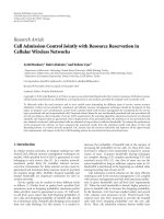
2.3. Transmission Strategy. A block diagram of transmis-
sion strategy for network MIMO coordination is shown
in Figure 1.Thetransmittedsymboltouserk is an n
r
-
dimensional vector u
k
, which is multiplied by an N
t
× n
r
precoding matrix W

k
and passed on to the base station’s
antenna array. Since all base station antennas are coordi-
nated, the complex antenna output vector x is composed of
signals for all K users. Therefore, x can be written as follows:
x
=
K

k=1
W
k
u
k
,
(5)
where
E[u
k
u
H
k
] = I
n
r
.Thereceivedsignaly
k
at user k can be
represented as
y

k
= H
k
W
k
u
k
+

j
/
=k
H
k
W
j
u
j
+ z
k
,(6)
where z
k
∼ CN (0,I
n
r
) denotes the normalized AWGN
vector at user k. The random characteristics of channel
matrix entries of H
k

are discussed in Section 4.They
encompass three factors: path loss, Rayleigh fading, and
lognormal shadowing. Random structure of the channel
coefficients ensures rank(H
k
) = min(n
r
, N
t
) = n
r
for user
k with probability one. Per-antenna power constraints (2)
impose a power constraint
[
S
x
]
i,i
=
E

xx
H

i,i
=
⎡
⎣
K


k=1
W
k
W
H
k
⎤
⎦
i,i
≤ p
i
, i = 1, , N
t
(7)
on each transmit antenna. The sum power constraint also
can be expressed as
tr
{S
x
}=
K

k=1
tr

W
k
W
H

k

≤
P. (8)
Due to the structure of multiuser zero forcing scheme,
the number of users that can be served simultaneously in
each time slot is limited. Hence, user selection algorithm
is necessary. We consider two main criteria for the user
selection scheme: maximum sum rate (MSR) and propor-
tional fairness (PF). We employ the greedy user selection
algorithm discussed in [43, 44]. The proportionally fair
user selection algorithm is based on greedy weighted user
selection algorithm with an update of the weights discussed
in [45–47].
3. Multicell Multiuser Block Diagonalization
To remove the intracluster interference, a practical linear zero
forcing can be employed. Applying multiuser zero forcing
to multiple-antenna users requires block diagonalization
(BD) rather than channel inversion [24]. Assuming the
transmission strategy in Section 2.3, each user’s data u
k
is
precoded with the matrix W
k
,suchthat
H
k
W
j
= 0 ∀k

/
= j,1≤ k, j ≤ K. (9)
Hence the received signal for user k can be simplified to
y
k
= H
k
W
k
u
k
+ n
k
. (10)
4 EURASIP Journal on Wireless Communications and Networking
u
1
u
2
u
K
User scheduling
n
r
W
1
W
2
W
K

Coordination


K
k
=1
W
k
W
H
k

ii
≤ p
i
i = 1, ,N
t
Intercluster interference
cancelation
.
.
.
.
.
.
.
.
.
.
.

.
BS
B
BS
2
BS
1
x
1
x
K
N
t
N
t
N
t
x
n
t
N
t
n
t
H
1
H
2
H
K

F
1
F
2
F
K
n
1
n
2
n
K
n
r
n
r
n
r
y
1
y
2
y
K
n
r
n
r
n
r

r
K
r
2
r
K
Figure 1: Block diagram of network MIMO coordination transmission strategy.
Let

H
k
= [H
T
1
···H
T
k
−1
H
T
k+1
···H
T
K
]
T
. Zero-interference
constraint in (9)forcesW
k
to lie in the null space of


H
k
which
requires a dimension condition Bn
t
≥ Kn
r
to be satisfied.
This directly comes from the definition of null space in linear
algebra [48]. Hence, the maximum number of users that can
be served in a time slot is K
= (N
t
/n
r
). We focus on the
K users which are selected through a scheduling algorithm
and assigned to one subband. The remaining unserved users
are referred to other subbands or will be scheduled in other
time slots. Recall that the vectors in (5)arenormalized
with respect to the standard deviation of the additive noise
component, σ,resultinginn
k
having components with unit
variance. Assume that

H
k
is a full rank matrix rank(


H
k
) =
(K − 1)n
r
, which holds with probability one due to the
randomness of entries of channel matrices. We perform
singular value decomposition (SVD)

H
k
= U
k
Λ
k
[
Υ
k
V
k
]
T
, (11)
where Υ
k
holds the first (K − 1)n
r
right singular vectors
corresponding to nonzero singular values and V

k
∈ C
N
t
×m
r
contains the last m
r
= N
t
− (K − 1)n
r
right singular vectors
corresponding to zero singular values of

H
k
.Ifnumberof
scheduled users is K
= N
t
/n
r
,thenm
r
= n
r
,otherwisem
r
>

n
r
when K<N
t
/n
r
. The orthonormality of V
k
means that
V
H
k
V
k
= I
m
r
. The columns of V
k
form a basis set in the null
space of

H
k
, and hence W
k
can be any linear combination of
the columns of V
k
,thatis,

W
k
= V
k
Ψ
k
, k = 1, , K, (12)
where Ψ
k
∈ C
m
r
×n
r
can be any arbitrary matrix subject to
the per-antenna power constraints [34]. Conventional BD
scheme proposed in [24] assumes only linear combinations
of a diagonal form to simplify it to a power allocation
algorithm through water-filling. The conventional BD is
optimal only when sum power constraint is applied [49],
and it is not optimal under per-antenna power constraints
[27, 30, 31].
3.1. Conventional BD. In conventional BD [24], the sum
power constraint is applied to the throughput maximization
problem and further relaxed to a simple water-filling power
allocation algorithm. In this scheme, the linear combination
introduced in (12) is confined to have a form given by
Ψ
k
=


V
k
Θ
1/2
k
, k = 1, , K, (13)
where

V
k
∈ C
m
r
×n
r
is the right singular vector of the matrix
H
k
V
k
corresponding to its nonzero singular values. Hence,
the aggregate precoding matrix of the conventional scheme,
W
BD
,isdefinedas
W
BD
=


V
1

V
1
V
2

V
2
··· V
K

V
K

Θ
1/2
, (14)
where Θ
= bdiag [Θ
1
, , Θ
K
] is a diagonal matrix whose
elements scale the power transmitted into each of the
columns of W
BD
. The sum power constraint implies that
K


k=1
tr

V
k

V
k
Θ
k

V
H
k
V
H
k

=
K

k=1
tr{Θ
k
}. (15)
This relaxes the problem to optimization over the diagonal
terms of Θ, which can be interpreted as a power allocation
problem and solved through well-known water-filling algo-
rithm over the diagonal terms of Θ.However,thisformof

BD cannot be extended as an optimal precoder to the case of
per-antenna power constraints because

W
BD
W
H
BD

i,i
=

V
BD
ΘV
H
BD

i,i
/
=
[
Θ
]
i,i
,
(16)
where V
BD
= [V

1

V
1
V
2

V
2
··· V
K

V
K
]. Note that ith
diagonal term of the left side of (16) is a linear combination
of all entries of matrix Θ and not only the diagonal terms.
The selection of Θ as a diagonal matrix reduces the search
domain size of optimization and hence does not necessarily
lead to the optimal solution. Furthermore,

V
k
impacts the
diagonal terms of W
BD
W
H
BD
(i.e., transmission covariance

matrix), and therefore insertion of

V
k
not necessarily reduces
the required power allocated to each antenna. In addition it
adds K SVD operations to the precoding computation proce-
dure (one for each served users) to find

V
k
. Additionally, the
per-antenna power constraints do not allow the optimization
EURASIP Journal on Wireless Communications and Networking 5
15
20
25
Sum rate (bits/s/Hz/cell)
30
35
40
45
50
6 8 10 12 14 16 18 20
Number of users per cell
Conventional BD
Optimal BD
N
t
= 6

N
t
= 12
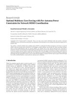
Figure 2: Comparison of sum rates for conventional BD versus the
proposed optimal BD for B
= 1, N
t
= 6, 12, n
r
= 2 using maximum
sum rate scheduling.
to lead to simple water-filling algorithm. Previous work
on BD with per-antenna (similarly with per-base-station)
power constraints for a case of multiple-receive antennas
employs this conventional BD and optimizes diagonal terms
of Θ [26–28]. Hence, it is not optimal. The optimal form
of BD proposed in this paper includes the optimization
over the entire null space of other users’ channel matrices
resulting in optimal precoders under per-antenna power
constraints, easily extendable to per-base station power
constraints.
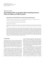
The numerical results in Figure 2 compare maximized
sum rate of a MIMO BC system using conventional BD
[24] with the optimal scheme proposed later in this paper.
There are 12 transmit antennas at the base station and 2
receive antennas at each mobile user. B
= 1isconsidered
to specifically show the difference between the two BD
schemes. Note that the conventional BD has a domain of
R

N
t
+
, while the optimal BD searches over all possible K
symmetric matrices and therefore has a larger domain of
C
Kn
r
(n
r
−1)/2
++
. Its size also grows with the number of users
per cell. Consequently, the difference between these two
schemes increases with the number of users per cell. Details
of the simulation setup are given in Section 4.Inthe
following section the optimal BD scheme is introduced and
discussed in detail, and the algorithm to find the precoders is
presented.
3.2. Optimal Multicell BD. The focus of this section is on
the design of optimal multicell BD precoder matrices W
k
to maximize the throughput while enforcing per-antenna
power constraints. In this scheme, we search over the entire
null space of other users channel matrices (

H
k
), that is, Ψ
k

can be any arbitrary matrix of C
m
r
×n
r
satisfying the per-
antenna power constraints.
Following the design of precoders according to (12), the
received signal for user k can be expressed as
y
k
= H
k
V
k
Ψ
k
u
k
+ z
k
.
(17)
Denote Φ
k
= Ψ
k
Ψ
H
k

∈ C
m
r
×m
r
, k = 1, , K,whichare
positive semidefinite matrices. The rate of kth user is given
by
R
k
= log



I + H
k
V
k
Φ
k
V
H
k
H
H
k



. (18)

Therefore, sum rate maximization problem can be expressed
as
maximize
K

k=1
log



I + H
k
V
k
Φ
k
V
H
k
H
H
k



subject to
⎡
⎣
K


k=1
V
k
Φ
k
V
H
k
⎤
⎦
i,i
≤ p
i
, i = 1, , N
t
,
Φ
k
 0, k = 1, , K,
(19)
where the maximization is over all positive semidefinite
matrices Φ
1
, , Φ
K
with a rank constraint of rank(Φ
k
) ≤
n
r

. Notice that the objective function in (19)isconcave([48,
p. 466]), and the constraints are also affine functions [23].
Thus, the problem is categorized as a convex optimization
problem. We propose a gradient descent algorithm to find
the optimal BD precoders. We define G
k
= H
k
V
k
and
correspondingly its right pseudoinverse matrix as G
†
k
=
G
H
k
(G
k
G
H
k
)
−1
.LetQ
k
= V
k
G

−1
k
which is an N
t
× n
r
matrix,
and we perform the SVD Q
H
k
ΛQ
k
= U
k
Σ
k
U
H
k
. We introduce
the positive semidefinite matrices Ω
k
defined as
Ω
k
= U
k
[
Σ
k

−I
]
+
U
H
k
, (20)
where the operator [D]
+
= diag[max(0, d
1
), ,max(0,d
n
)]
on a diagonal matrix D
= diag [d
1
, , d
n
].
Theorem 1. The optimal BD precoders can be obtained
through solving the dual problem
minimize g
(
Λ
)
subject to Λ
 0, Λ diagonal,
(21)
where

g
(
Λ
)
=−
K

k=1
log



Q
H
k
ΛQ
k
−Ω
k



−
Kn
r
+tr
⎧
⎨
⎩
K


k=1

Q
H
k
ΛQ
k
−Ω
k

⎫
⎬
⎭
+tr{ΛP}
(22)
with a gradient descent direction given as
ΔΛ
=
K

k=1
diag

Q
k

Q
H
k

ΛQ
k
−Ω
k

−1
Q
H
k

−
P −
K

k=1
diag

Q
k
Q
H
k

.
(23)
6 EURASIP Journal on Wireless Communications and Networking
The optimal BD precoders for the optimal value of Λ

are given
as

W
k
= V
k

G
†
k


Q
H
k
Λ

Q
k
−Ω
k

−1
−I


G
†
k

H


1/2
. (24)
Proof. Theproofisgivenintheappendix.
The KKT conditions for the dual problem are given as
Λ
 0,
∇
Λ
g  0,
λ
i

∇
Λ
g

i,i
= 0, i = 1, ,N
t
(25)
with the last condition being the complementarity ([23,p.
142]). Thus, the stopping criterion for the gradient descent
method can be established using small values of

≥
0
replacing zero values.
More interestingly, the sum rate maximization in (19)
through the dual problem in (21) facilitates the extension
to any linear power constraints on the transmit antennas.

The dual problem has N
t
variables λ
i
, i = 1, , N
t
,onefor
each transmit antenna power constraint. More general power
constraints than those given in (19) can be defined as [31]
tr
⎧
⎨
⎩
K

k=1
V
k
Φ
k
V
H
k
T
l
⎫
⎬
⎭
≤
p

l
, l = 1, ,L, (26)
where T
l
are positive semidefinite symmetric matrices and
p
l
are nonnegative values corresponding to each of L linear
constraints. The special case of this structure of power
constraints has been discussed frequently in the literature:
for L
= 1, p
1
= P,andT
1
= I, the conventional sum power
constraint results [24]; when L
= N
t
and T
l
is a matrix with
its lth diagonal term equal to one and all other elements zero,
we get per-antenna power constraints studied in this section.
Another scenario is per-base station power constraint, which
is derived with L
= B, p
l
= P
l

(lth per-base power limit),
and T
l
all zero except equal to one on n
t
terms of its diagonal
each corresponding to one of the lth base station’s transmit
antennas. When the sum power constraint is applied only
one dual variable is needed in dual optimization problem
(21)(i.e.,Λ
= λI
N
t
), where λ determines the water level in
the water-filling algorithm [24]. For per-base station power
constraints, the optimization dual variable can be defined as
Λ
= Λ
bs
⊗I
n
t
,whereΛ
bs
= diag [λ
1
, , λ
B
] consists of B dual
variables (one for each base station) and the operator

⊗ is
the Kronecker product [48]. The details of the optimization
steps in the per-base station power constraints scenario are
discussed in Section 3.3, and the study of general linear
constraints is left for further work.
3.3. Per-Base-Station Power Constraints. In this Section, the
extension of the ZF beamforming optimization to the system
with per-base station power constraint is considered. The
optimization problem in (19)canberewrittenconsidering
the per-base-station power constraints as
maximize
K

k=1
log



I + H
k
V
k
Φ
k
V
H
k
H
H
k




subject to tr

Δ
b

K

k=1
V
k
Φ
k
V
H
k

≤
P
b
,
b
= 1, ,B, Φ
k
 0, k = 1, ,K,
(27)
where P
1

, , P
B
are the per-base station maximum powers
and Δ
b
is a diagonal matrix with its entries equal to one for
the corresponding antennas within the base-station b and the
rest equal to zero. For the simplicity, bth n
t
-entries of the
diagonal of Δ
b
are only equal to one. Following similar steps
as (A.1), the Lagrange dual function is obtained as
L
(
{S}, λ
)
=
K

k=1
log |I + S
k
|
−
B

b=1
tr

⎧
⎨
⎩
λ
b
Δ
b
⎛
⎝
K

k=1
Q
k
S
k
Q
H
k
−P
bs
⊗I
n
t
⎞
⎠
⎫
⎬
⎭
+

K

k=1
tr{Ω
k
S
k
},
(28)
where P
bs
= diag[P
1
, , P
B
]and⊗ is the Kronecker product
[48]. The KKT conditions yield that
S
k
=

Q
H
k

Λ
bs
⊗I
n
t


Q
k
−Ω
k

−1
−I, k = 1, ,K,
(29)
where Λ
bs
= diag [λ
1
, , λ
B
]andΩ
k
can be defined in
a similar way as (20). The dual problem can be expressed
similarly to (21). Following the steps in Section 3.2,the
gradient descent search direction is given by
∇
Λ
g
=−
K

k=1
diag
b=1, ,B


tr
b

Q
k

Q
H
k

Λ
bs
⊗I
n
t

Q
k
−Ω
k

−1
Q
H
k

+ P
bs
+

K

k=1
diag
b=1, ,B

tr
b

Q
k
Q
H
k

,
(30)
where tr
b
is a partial matrix trace over bth n
t
-entries of the
diagonal terms of a matrix. diag
b=1, ,B
[·]givesadiagonal
matrix with B elements computed for each b
= 1, ,B.
3.4. Single-Antenna Receivers. Although this paper studies a
network MIMO system with multiple receive antenna users,
the results can be applied to a system with single receive

antenna users. In this case each user’s transmission must be
orthogonal to a vector (rather than a matrix), which is the
basis vector for other users’ transmissions. The optimization
EURASIP Journal on Wireless Communications and Networking 7
is over all real vectors with positive elements (
R
N
t
+
) satisfying
the power constraints. This approach facilitates the optimiza-
tion presented in [30, 31] using the generalized inverses and
multistep optimizations.
4. Simulation Setup
The propagation model between each base station’s transmit
antenna and mobile user’s receive antenna includes three
factors: a path loss component proportional to d
−β
kb
(where
d
kb
denotes distance from base station b to mobile user k
and β
= 3.8 is the path loss exponent) and two random
components representing lognormal shadow fading and
Rayleigh fading. The channel gain between transmit antenna
t of the base station b and receive antenna r of the kth user is
given by


H
k,b

(r,t)
= α
(r,t)
k,b




ρ
k,b

d
kb
d
0

−β
Γ
, (31)
where [H
k,b
]
(r,t)
is the (r,t)th element of the channel matrix
H
k,b
∈ C

n
r
×n
t
from the base station b tothemobileuserk,
α
(r,t)
k,b
∼ CN (0, 1) represents independent Rayleigh fading,
d
0
= 1 km is the cell radius, and ρ
k,b
= 10
ρ
(dBm)
k,b
/10
is the
lognormal shadow fading variable between bth base station
and kth user, where ρ
(dBm)
k,b
∼ CN (0,σ
ρ
)andσ
ρ
= 8dBisits
standard deviation. A reference SNR, Γ
= 20dB, is a typical

value of the interference-free SNR at the cell boundary (as in
[7, 38]).
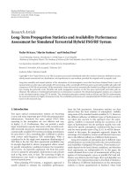
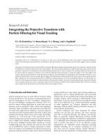
Our cellular network setup involves clustering. Since
global coordination is not feasible, clustering with cluster
sizes of up to B
= 7 is considered. The cellular network
layoutisshowninFigure3. A base station is located
at the center of each hexagonal cell. Each base station is
equipped with n
t
transmit antennas. There are n
r
receive
antennas on each user’s receiver, and there are K users per
cell per subband. All N
t
= Bn
t
base stations’ transmit
antennas in each cluster are coordinated. In Figure 3 the
clusters of sizes 3 and 7 are shown. For cluster size 7, one
wrap-around layer of clusters is considered to contribute
inter-cluster interference, while for B
= 3twotiers
of interfering cells are accounted for. User locations are
generated randomly, uniformly, and independently in each
cell. For each drop of users, the distance of users from
base stations in the network is computed, and path loss,
lognormal, and Rayleigh fading are included in the channel
gain calculations. User scheduling is performed employing

a greedy algorithm with maximum sum rate (MSR) and
proportionally fair (PF) criteria with the updated weights
for the rate of each user as in [45–47]. To compare the
results all the sum rates achieved through network MIMO
coordination are normalized by the size of clusters B.Base
stations causing inter-cluster interference are assumed to
transmit at full power, which is the worst case as discussed
in Section 2.
Figure 3: The cellular layout of B = 3andB = 7 clustered
network MIMO coordination. The borders of clusters are bold.
Green colored cells represent the analyzed center cluster, and the
grey cells are causing intercell interference. For B
= 7onetier
of interfering clusters is considered, while for B
= 3twotiersof
interfering cells are accounted for.
5. Numerical Results
In this section, the performance results (obtained via Monte
Carlo simulations) of the proposed optimal BD scheme
in a network MIMO coordinated system are discussed.
The network MIMO coordination exhibits several system
advantages, which are exposed in the following.
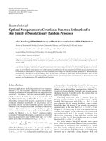
5.1. Network MIMO Gains. While the universal network
MIMO coordination is practically impossible, clustering is
a practical scheme, which also benefits the network MIMO
coordination gains and reduces the amount of feedback
required at the base stations [26, 38]. The size of clusters,
B, is a parameter in network MIMO coordination. B
= 1
means no coordination with optimal BD scheme applied.

Figure 4 shows that with increasing cluster size throughput
of the system increases. System throughput is computed
using MSR scheduling and averaged over several channel
realizations for a large number of user locations generated
randomly. The normalized throughput for different cluster
sizes is compared, which means that the total throughput in
each cluster is divided by the number of cells in each cluster
B. The normalized sum rate has lower variance in larger
clusters, which shows that the performance of the system
is less dependent on the position of users and that network
MIMO coordination brings more stability to the system.
5.2. Multiple-Antenna Gains. The intercell interference mit-
igation through coordination of base stations enables the
cellular network to enjoy the great spectral efficiency
improvement associated with employing multiple antennas.
Figure 5 shows the linear growth of the maximum through-
put achievable through the proposed optimal multicell BD
8 EURASIP Journal on Wireless Communications and Networking
0
0.1
0.2
0.3
0.4
CDF
0.5
0.6
0.7
0.8
0.9
1

5 1015202530354045
Sum rate (bps/Hz/cell)
DPC
Optimal BD
B
= 3
B
= 7
B
= 1
No coordination
Figure 4: CDF of sum rate with different cluster sizes B = 1,3,7;
n
t
= 4, n
r
= 2, and 10 users per cell.
15
20
25
Sum rate (bits/s/Hz/cell)
30
35
40
45
50
60
55
2 4 6 8 10 12
n

t
DPC
Optimal BD
B
= 1
B
= 3
B
= 3
Figure 5: Sum rate increase with the number of antennas per-base
station n
r
= 2.
and the capacity limits of DPC [22]. The number of receive
antennas at each mobile user is fixed to n
r
= 2, and
the number of transmit antennas n
t
at each base station
is increasing. When the cluster size grows, the slope of
spectral efficiency also increases. The maximum power on
each transmit antenna is normalized such that the total
power at each base station for different n
t
is constant.
5.3. Multiuser Diversity. Multicell coordination benefits
from increased multiuser diversity, since the number of users
scheduled at each time interval is B times of that without
coordination. In Figure 6, the multiuser diversity gain of

network MIMO is shown with up to 10 users per cell.
The MSR scheduling is applied for each drop of users and
averaged over several channel realizations.
8
10
12
Sum rate (bits/s/Hz/cell)
14
16
18
20
22
24
26
30
28
23 456 87910
Number of users per cells
DPC
Optimal BD
B
= 1
B
= 7
B
= 3
Figure 6: Sum rate per cell achieved with the proposed optimal BD
and the capacity limits of DPC for cluster sizes B
= 1, 3,7; n
t

= 4,
n
r
= 2.
5.4. Fairness Advantages. One of the main purposes of
network MIMO coordination is that the cell-edge users gain
from neighboring base stations signals. In Figure 7,the
cumulative distribution functions (CDFs) of the mean rates
for the users are shown and compared for B
= 1(i.e.,
beamforming without coordination) and B
= 3, 7 using the
proposed optimal BD scheme. There are 10 users per cell
randomly and uniformly dropped in the network for each
simulation. For each drop of users, the proportionally fair
scheduling algorithm is applied over hundreds of scheduling
time intervals using sliding window width τ
= 10 time slots
(see [17]). Each user’s rates achieved in all time intervals
are averaged to find the mean rates per user, and their
corresponding CDF for several user locations is plotted.
As shown by the plots, for B
= 3andB = 7network
MIMO coordination nearly 70% and 80% users have mean
rate larger than 1 bps/Hz, respectively, while for the scheme
without coordination it is only 45% of the users. However,
fairness among users does not seem to be improved when
cluster sizes increase. This is perhaps due to the existence of
larger number of cell-edge users when cluster size increases.
5.5. Convergence. Convergence of the gradient descent

method proposed in Section 3.2 is illustrated in Figure 8.
The normalized sum rates obtained after each iteration
with respect to the optimal target values versus the number
of iterations are depicted. The convergence behavior of
the algorithm for 20 independent and randomly generated
user location sets is shown, and their channel realizations
are tested with the proposed iterative algorithm, and the
values of sum rate after each iteration divided by the target
value are monitored. For nearly all system realizations, the
optimizations converge to the target valuewithin only 10 first
iterations with 1% error.
EURASIP Journal on Wireless Communications and Networking 9
0
0.1
0.2
0.3
0.4
CDF
0.5
0.6
0.7
0.8
0.9
1
00.511.522.533.54
Rate (bits/s/Hz)
B
= 3
B
= 7

B
= 1
No coordination
Figure 7: CDF of the mean rates in the clusters of sizes B = 3, 7
and comparison with B
= 1 (no coordination) using the proposed
optimal BD.
0.92
0.94
0.96
0.98
Rate/target value
1
1.02
1.04
1.06
1.08
1.1
1.12
12345 6 8 10 15 20 25
Number of iterations
Figure 8: Convergence of the gradient descent method for the
proposed optimal BD for B
= 3; n
t
= 4, n
r
= 2, and 8 users per
cell.
6. Conclusions

In this paper, a multicell coordinated downlink MIMO
transmission has been considered under per-antenna power
constraints. Suboptimality of the conventional BD consid-
ered in earlier research has been shown, and this has moti-
vated the search for the optimal BD scheme. The optimal
block diagonalization (BD) scheme for network MIMO
coordinated system under per-antenna power constraints has
been proposed in the paper, and it has been shown that
it can be generalized to the case of per-base station power
constraints. A simple iterative descent gradient algorithm
has also been proposed in the paper, which determines
the optimal precoders for multicell BD. The comprehensive
simulation results have demonstrated advantages achieved
by using multicell coordinated transmission under more
practical per-antenna power constraints.
Appendix
A. Proof of Theorem 1
We consider the optimization problem (19). For the ease of
further analysis, let us substitute S
k
= H
k
V
k
Φ
k
V
H
k
H

H
k
and
G
k
= H
k
V
k
,whererank(G
k
) ≤ n
r
. Note that the rank
constraint on Φ
k
must be inserted into the optimization
when m
r
>n
r
, and hence it makes the problem nonconvex.
Thus, to analyze this problem two cases are considered based
on the value of m
r
with respect to n
r
. In the first case
m
r

= n
r
, when the total number of transmit antennas at
all base stations, N
t
, is equal to the total number of receive
antennas at all K served users, N
r
. In the second case N
t
>
N
r
.
A.1. (N
t
= N
r
). This happens when exactly K = N
t
/n
r
users
are scheduled. In this case, the rank constraint over Φ
k
can
be dropped because m
r
= n
r

, and therefore the optimization
problem in (19)isconvex.ThematricesG
k
are also square
and invertible. Therefore G
†
k
= G
−1
k
.LetQ
k
= V
k
G
−1
k
which
is an N
t
× n
r
matrix. Thus, the throughput maximization
problem can be expressed as (since S
k
 0 ⇔ G
−1
k
S
k

G
−H
k
)
maximize
K

k=1
log|I + S
k
|
subject to
⎡
⎣
K

k=1
Q
k
S
k
Q
H
k
⎤
⎦
i,i
≤ P
i
, i = 1, , N

t
S
k
 0, k = 1, , K,
(A.1)
where S
k
∈ C
n
r
×n
r
. Although one possibility is to perform
this convex optimization with Kn
r
(n
r
−1)/2 variables intro-
ducing logarithmic barrier functions for inequality power
constraints and the set of positive semidefinite constraints,
we approach the problem by establishing the dual problem
and solving it through simple and efficient gradient descent
method [23]. Hence, the Lagrangian function can be formed
as
L
(
{S}; Λ
)
=
K


k=1
log |I + S
k
|+
K

k=1
tr{Ω
k
S
k
}
−
tr
⎧
⎨
⎩
Λ
⎛
⎝
K

k=1
Q
k
S
k
Q
H

k
−P
⎞
⎠
⎫
⎬
⎭
,
(A.2)
where Λ
= diag(λ
1
, , λ
N
t
) is a dual variable which is a
diagonal matrix with nonnegative elements, λ
i
≥ 0. The
positive semidefinite matrix Ω
k
is a dual variable to assure
positive semidefiniteness of S
k
.TheKarush-Kuhn-Tucker
10 EURASIP Journal on Wireless Communications and Networking
(KKT) conditions require that the optimal values of primal
and dual variables [23] satisfy the following:
S
k

=

Q
H
k
ΛQ
k
−Ω
k

−1
−I, S
k
 0,
tr
{Ω
k
S
k
}=0, Ω
k
 0,
tr
⎧
⎨
⎩
Λ
⎛
⎝
K


k=1
Q
k
S
k
Q
H
k
−P
⎞
⎠
⎫
⎬
⎭
=
0, Λ  0
P
 diag
⎡
⎣
K

k=1
Q
k
S
k
Q
H

k
⎤
⎦
.
(A.3)
Let the SVD of Q
H
k
ΛQ
k
= U
k
Σ
k
U
H
k
.SinceQ
H
k
ΛQ
k
 0, the
diagonal entries of Σ
k
are the eigenvalues of Q
H
k
ΛQ
k

.Thefirst
KKT condition on S
k
and Ω
k
requires that
Ω
k
= U
k
[
Σ
k
−I
]
+
U
H
k
,
(A.4)
where the operator [D]
+
= diag[max(0, d
1
), ,max(0,d
n
)]
on a diagonal matrix D
= diag[d

1
, , d
n
]. Replacing these in
the KKT condition corresponding to the power constraints
gives
tr
⎧
⎨
⎩
Λ
⎛
⎝
K

k=1
Q
k
S
k
Q
H
k
−P
⎞
⎠
⎫
⎬
⎭
=

Kn
r
−tr{ΛP}−tr
⎧
⎨
⎩
K

k=1

Q
H
k
ΛQ
k
−Ω
k

⎫
⎬
⎭
.
(A.5)
Now, we establish the Lagrange dual function as
g
(
Λ
)
= sup
S

k
L
(
{S}
)
=−
K

k=1
log



Q
H
k
ΛQ
k
−Ω
k



−
Kn
r
+tr
⎧
⎨
⎩

K

k=1

Q
H
k
ΛQ
k
−Ω
k

⎫
⎬
⎭
+tr{ΛP}.
(A.6)
Since the constraint functions are affine, strong duality holds,
and thus the dual objective reaches a minimum at the
optimal value of the primal problem [23]. As a result, the
Lagrange dual problem can be stated as
minimize g
(
Λ
)
subject to Λ
 0, Λ diagonal.
(A.7)
The gradient of g can be obtained from (A.6)as
∇

Λ
g =−
K

k=1
diag

Q
k

Q
H
k
ΛQ
k
−Ω
k

−1
Q
H
k

+ P +
K

k=1
diag

Q

k
Q
H
k

.
(A.8)
This gives a descent search direction, ΔΛ
=−∇
Λ
g,forthe
gradient algorithm for the Lagrange dual problem [23].
A.2. N
t
>N
r
. When the total number of transmit antennas
is strictly larger than the total number of receive antennas in
the network (i.e., N
t
>N
r
) the optimization problem in (A.1)
is no longer convex due to the rank constraints. We relax the
problem and show that it leads to an optimal solution, which
also satisfies the rank constraints in the original problem.
Similar gradient algorithm to the one for N
t
= N
r

can be
deployed to find the optimal BD precoders.
Recall that m
r
= N
t
− (K − 1)n
r
.Thus,whenthe
total number of transmit antennas is strictly larger than the
total number of receive antennas, N
t
>N
r
,thenm
r
>n
r
.
From Section 3 note that V
k
is an N
t
× m
r
matrix, and
correspondingly the size of Ψ
k
is m
r

× n
r
which enforces a
rank constraint over Φ
k
= Ψ
k
Ψ
H
k
.(i.e.,rank(Φ
k
) ≤ n
r
).
This updates the optimization in (19) by adding the rank
constraints as
maximize
K

k=1
log



I + H
k
V
k
Φ

k
V
H
k
H
H
k



subject to
⎡
⎣
K

k=1
V
k
Φ
k
V
H
k
⎤
⎦
i,i
≤ p
i
, i = 1, , N
t

Φ
k
 0, rank
(
Φ
k
)
≤ n
r
, k = 1, , K.
(A.9)
Theproblemaboveisnotconvexduetotherankconstraint.
Assume the convex relaxation problem obtained by remov-
ing the rank constraint. The problem can then be expressed
as
maximize
K

k=1
log



I + H
k
V
k
Φ
k
V

H
k
H
H
k



subject to
⎡
⎣
K

k=1
V
k
Φ
k
V
H
k
⎤
⎦
i,i
≤ p
i
, i = 1, , N
t
Φ
k

 0, k = 1, ,K.
(A.10)
Since this problem is convex and the constraints are affine,
any solution satisfying the KKT conditions is optimal [23].
Let us introduce an optimization problem
maximize
K

k=1
log|I + S
k
|
subject to
⎡
⎣
K

k=1
V
k
G
†
k
S
k

G
†
k


H
V
H
k
⎤
⎦
i,i
≤ p
i
, i = 1, , N
t
,
S
k
 0, k = 1, ,K.
(A.11)
Assume that the optimal solutions for this problem are
S

k
s. Defining Φ
k
= G
†
k
S

k
(G
†

k
)
H
satisfies all the KKT
conditions for (A.10), since G
k
Φ
k
G
H
k
= S

k
.Furthermore,
rank(Φ
k
) =rank(S
k
) ≤ n
r
which also satisfies the rank
constraint in the original optimization problem (A.9). Note
that also Φ
k
 0 ⇔ S

k
 0(see[48, p. 399] ).
EURASIP Journal on Wireless Communications and Networking 11

The optimization in (A.11)isequivalenttotheconvex
optimization problem in (A.1)byreplacingQ
k
= V
k
G
†
k
.
Recall that when m
r
= n
r
then the matrix G
k
is square and
invertible. Hence, Q
k
= V
k
G
−1
k
, as defined in Section A.1.
Thus, this problem can be solved through the gradient
descent method applied to the dual problem (A.7)with
the gradient descent search direction (A.8). The stopping
criterion is also the same as (25)exceptthatQ
k
has different

definition.
Note that (24) can be simply concluded from the first
equation of the KKT conditions (A.3) and the definition of
Φ
k
= G
†
k
S

k
(G
†
k
)
H
for the optimal value of dual variables Λ

.
Acknowledgments
Funding for this paper has been provided by the Natural
Sciences and Engineering Research Council (NSERC) of
Canada, TRLabs, the Rohit Sharma Professorship, Alberta
Innovates Technology Futures, and the University of Alberta.
The work discussed in this paper was presented in part at the
WCNC 2008, Las Vegas, USA, March-April 2008.
References
[1] G. J. Foschini and M. J. Gans, “On limits of wireless com-
munications in a fading environment when using multiple
antennas,” Wireless Personal Communications,vol.6,no.3,pp.

311–335, 1998.
[2] E. Telatar, “Capacity of multi-antenna Gaussian channels,”
European Transactions on Telecommunications, vol. 10, no. 6,
pp. 585–595, 1999.
[3] D. Gesbert, M. Kountouris, R. W. Heath, C. B. Chae, and T.
S
¨
alzer, “Shifting the MIMO paradigm,” IEEE Signal Processing
Magazine, vol. 24, no. 5, pp. 36–46, 2007.
[4] R. S. Blum, “MIMO capacity with interference,” IEEE Journal
on Selected Areas in Communications, vol. 21, no. 5, pp. 793–
801, 2003.
[5]H.Dai,A.F.Molisch,andH.V.Poor,“Downlinkcapacity
of interference-limited MIMO systems with joint detection,”
IEEE Transactions on Wireless Communications,vol.3,no.2,
pp. 442–453, 2004.
[6] M. K. Karakayali, G. J. Foschini, R. A. Valenzuela, and R.
D. Yates, “On the maximum common rate achievable in a
coordinated network,” in Proceedings of the IEEE I nternational
Conference on Communications (ICC ’06), pp. 4333–4338,
Istanbul, Turkey, June 2006.
[7] G. J. Foschini, K. Karakayali, and R. A. Valenzuela, “Coor-
dinating multiple antenna cellular networks to achieve enor-
mous spectral efficiency,” IEE Proceedings: Communications,
vol. 153, no. 4, pp. 548–555, 2006.
[8] O. Somekh, B. M. Zaidel, and S. Shamai, “Sum rate characteri-
zation of joint multiple cell-site processing,” IEEE Transactions
on Information Theory, vol. 53, no. 12, pp. 4473–4497, 2007.
[9] H. Zhang and H. Dai, “Cochannel interference mitigation
and cooperative processing in downlink multicell multiuser

MIMO networks,” EURASIP Journal on Wireless Communica-
tions and Networking, vol. 2004, no. 2, pp. 222–235, 2004.
[10]S.Jing,D.N.C.Tse,J.B.Soriaga,J.Hou,J.E.Smee,
and R. Padovani, “Downlink macro-diversity in cellular
networks,” in Proceedings of the IEEE International Symposium
on Information Theory (ISIT ’07), pp. 1–5, Nice, France, June
2007.
[11] D. Gesbert, S. Hanly, H. Huang, S. Shamai Shitz, O. Simeone,
and W. Yu, “Multi-cell MIMO cooperative networks: a new
look at interference,” IEEE Journal on Selected Areas in
Communications, vol. 28, no. 9, pp. 1380–1408, 2010.
[12] S. Shamai and B. M. Zaidel, “Enhancing the cellular down-
link capacity via co-processing at the transmitting end,” in
Proceedings of the 53rd IEEE Vehicular Technology Conference
(VTC ’01-Spring), vol. 3, pp. 1745–1749, Rhodes, Greece, May
2001.
[13] A. Goldsmith, S. A. Jafar, N. Jindal, and S. Vishwanath,
“Capacity limits of MIMO channels,” IEEE Journal on Selected
Areas in Communications, vol. 21, no. 5, pp. 684–702, 2003.
[14] S. A. Jafar, G. J. Foschini, and A. J. Goldsmith, “PhantomNet:
exploring optimal multicellular multiple antenna systems,”
EURASIP Journal on Applied Signal Processing, vol. 2004, no.
5, pp. 591–604, 2004.
[15] W. Choi and J. G. Andrews, “The capacity gain from intercell
scheduling in multi-antenna systems,” IEEE Transactions on
Wireless Communications, vol. 7, no. 2, pp. 714–725, 2008.
[16] G. Caire and S. Shamai, “On the achievable throughput of a
multiantenna Gaussian broadcast channel,” IEEE Transactions
on Information Theory, vol. 49, no. 7, pp. 1691–1706, 2003.
[17] P. Viswanath and D. N. C. Tse, “Sum capacity of the vector

Gaussian broadcast channel and uplink-downlink duality,”
IEEE Transactions on Information Theory,vol.49,no.8,pp.
1912–1921, 2003.
[18]W.YuandJ.M.Cioffi, “Sum capacity of Gaussian vector
broadcast channels,” IEEE Transactions on Information Theory,
vol. 50, no. 9, pp. 1875–1892, 2004.
[19] H. Weingarten, Y. Steinberg, and S. Shamai, “The capacity
region of the Gaussian multiple-input multiple-output broad-
cast channel,” IEEE Transactions on Information Theory,vol.
52, no. 9, pp. 3936–3964, 2006.
[20]S.Vishwanath,N.Jindal,andA.Goldsmith,“Duality,
achievable rates, and sum-rate capacity of Gaussian MIMO
broadcast channels,” IEEE Transactions on Information Theory,
vol. 49, no. 10, pp. 2658–2668, 2003.
[21] W. Yu, “Uplink-downlink duality via minimax duality,” IEEE
Transactions on Information Theory, vol. 52, no. 2, pp. 361–
374, 2006.
[22] W. Yu and T. Lan, “Transmitter optimization for the multi-
antenna downlink with per-antenna power constraints,” IEEE
Transactions on Signal Processing, vol. 55, no. 6, pp. 2646–2660,
2007.
[23] S. Boyd and L. Vandenberghe, Convex Optimization,Cam-
bridge University Press, New York, NY, USA, 2004.
[24] Q. H. Spencer, A. L. Swindlehurst, and M. Haardt, “Zero-
forcing methods for downlink spatial multiplexing in mul-
tiuser MIMO channels,” IEEE Transactions on Sig nal Process-
ing, vol. 52, no. 2, pp. 461–471, 2004.
[25] L U. Choi and R. D. Murch, “A transmit preprocessing tech-
nique for multiuser MIMO systems using a decomposition
approach,” IEEE Transactions on Wireless Communications,

vol. 3, no. 1, pp. 20–24, 2004.
[26] J.Zhang,R.Chen,J.G.Andrews,A.Ghosh,andR.W.Heath,
“Networked MIMO with clustered linear precoding,” IEEE
Transactions on Wireless Communications,vol.8,no.4,pp.
1910–1921, 2009.
[27] K. Karakayali, R. Yates, G. Foschini, and R. Valenzuela, “Opti-
mum zero-forcing beamforming with per-antenna power con-
straints,” in Proceedings of the IEEE International Symposium
on Information Theory (ISIT ’07), pp. 101–105, Nice, France,
June 2007.
12 EURASIP Journal on Wireless Communications and Networking
[28] Y. Hadisusanto, L. Thiele, and V. Jungnickel, “Distributed
base station cooperation via block-diagonalization and dual-
decomposition,” in Proceedings of the IEEE Global Telecommu-
nications Conference (GLOBECOM ’08), pp. 3539–3543, New
Orleans, USA, December 2008.
[29] W. Liu, S. X. Ng, and L. Hanzo, “Multicell cooperation based
SVD assisted multi-user MIMO transmission,” in Proceedings
of the 69th I EEE Vehicular Technology Conference (VTC ’09-
Spring), Barcelona, Spain, April 2009.
[30] A.Wiesel,Y.C.Eldar,andS.Shamai,“Zero-forcingprecoding
and generalized inverses,” IEEE Transactions on Signal Process-
ing, vol. 56, no. 9, pp. 4409–4418, 2008.
[31] H. Huh, H. Papadopoulosy, and G. Caire, “MIMO broadcast
channel optimization under general linear constraints,” in
Proceedings of the IEEE International Symposium on Informa-
tion Theory (ISIT ’09), pp. 2664–2668, Seoul, Korea, June-July
2009.
[32] F. Boccardi and H. Huang, “Zero-forcing precoding for
the MIMO broadcast channel under per-antenna power

constraints,” in Proceeding s of the 7th IEEE Workshop on Signal
Processing Advances in Wireless Communications (SPAWC ’06),
Cannes, France, July 2006.
[33] L. Vandenberghe, S. Boyd, and S. P. Wu, “Determinant max-
imization with linear matrix inequality constraints,” SIAM
Journal on Matrix Analysis and Applications,vol.19,no.2,pp.
499–533, 1998.
[34] S. Kaviani and W. A. Krzymie
´
n, “Sum rate maximization
of MIMO broadcast channels with coordination of base
stations,” in Proceedings of the IEEE Wireless Communications
and Networking Conference (WCNC ’08), pp. 1079–1084, Las
Vegas, USA, March-April 2008.
[35] R. Zhang, “Cooperative multi-cell block diagonalization with
per-base-station power constraints,” IEEE Journal on Selected
Areas in Communications, vol. 28, no. 9, pp. 1435–1445, 2010.
[36] S. Boyd, L. Xiao, and A. Mutapcic, “Subgradient methods,”
lecture notes of EE392o, Stanford University, Autumn Quarter
2003-2004.
[37] M.K.Karakayali,R.D.Yates,andL.V.Razoumov,“Downlink
throughput maximization in CDMA wireless networks,” IEEE
Transactions on Wireless Communications,vol.5,no.12,pp.
3492–3500, 2006.
[38] H. Huang, M. Trivellato, A. Hottinen, M. Shafi, P. J. Smith, and
R. Valenzuela, “Increasing downlink cellular throughput with
limited network MIMO coordination,” IEEE Transactions on
Wireless Co mmunications, vol. 8, no. 6, pp. 2983–2989, 2009.
[39] S. Venkatesan, “Coordinating base stations for greater uplink
spectral efficiency in a cellular network,” in Proceeding s of the

18th Annual IEEE International Symposium on Personal, Indoor
and Mobile Radio Communications (PIMRC ’07),Athens,
Greece, September 2007.
[40] T. M. Cover and J. A. Thomas, Elements of Information Theory,
Wiley, New York, NY, USA, 1991.
[41]S.YeandR.S.Blum,“Somepropertiesofthecapacityof
MIMO systems with co-channel interference,” in Proceedings
of the IEEE International Conference on Acoustics, Speech,
and Signal Processing (ICASSP ’05), vol. 3, pp. 1153–1156,
Philadelphia, USA, March 2005.
[42]S.Shim,J.S.Kwak,R.W.Heath,andJ.G.Andrews,
“Block diagonalization for multi-user MIMO with other-cell
interference,” IEEE Transactions on Wireless Communicat ions,
vol. 7, no. 7, pp. 2671–2681, 2008.
[43] G. Dimi
´
c and N. D. Sidiropoulos, “On downlink beamforming
with greedy user selection: performance analysis and a simple
new algorithm,” IEEE Transactions on Signal Processing, vol. 53,
no. 10, pp. 3857–3868, 2005.
[44] Z. Shen, R. Chen, J. G. Andrews, R. W. Heath Jr., and
B. L. Evans, “Low complexity user selection algorithms for
multiuser MIMO systems with block diagonalization,” IEEE
Transactions on Signal Processing, vol. 54, no. 9, pp. 3658–3663,
2006.
[45] H. Viswanathan, S. Venkatesan, and H. Huang, “Down-
link capacity evaluation of cellular networks with known-
interference cancellation,” IEEE Journal on Selected Areas in
Communications, vol. 21, no. 5, pp. 802–811, 2003.
[46] S. Sigdel and W. A. Krzymie

´
n, “Simplified fair scheduling and
antenna selection algorithms for multiuser MIMO orthogonal
space-division multiplexing downlink,” IEEE Transactions on
Vehicular Technology, vol. 58, no. 3, pp. 1329–1344, 2009.
[47] S. Sigdel and W. A. Krzymie
´
n, “Simplified channel-aware
greedy scheduling and antenna selection algorithms for
multiuser MIMO systems employing orthogonal space divi-
sion multiplexing,” in Advances in Mobile and Wireless
Communications—Views of the 16th IST Mobile and Wireless
Communication Summit, chapter 2, pp. 23–51, Springer,
Heidelberg, Germany, 2008.
[48] R. A. Horn and C. R. Johnson, Matrix Analysis,Cambridge
University Press, Cambridge, UK, 1985.
[49] S. Kaviani and W. A. Krzymie
´
n, “On the optimality of mul-
tiuser zero-forcing precoding in MIMO broadcast channels,”
in Proceedings of the 69th IEEE Vehicular Technology Conference
(VTC ’09-Spring), Barcelona, Spain, April 2009.