Báo cáo hóa học: " Research Article A Novel Approach to Detect Network Attacks Using G-HMM-Based Temporal Relations between Internet Protocol Packets" pot

Hindawi Publishing Corporation
EURASIP Journal on Wireless Communications and Networking
Volume 2011, Article ID 210746, 14 pages
doi:10.1155/2011/210746
Research Ar ticle
A Novel Approach to Detect Network Attacks
Using G-HMM-Based Temporal Relations between
Internet Protocol Packets
Taeshik Shon,
1
Kyusuk Han,
2
James J. (Jong Hyuk) Park,
3
and Hangbae Chang
4
1
Division of Information and Computer Engineering, College of Information Technology, Ajou University,
Suwon 443-749, Republic of Korea
2
Depart ment of Information and Communication Engineering, Korea Advanced Institute of Science and Technology, 119 Munjiro,
Yuseong-gu, Daejeon 305-701, Republic of Korea
3
Depart ment of Computer Science and Engineering, Seoul National University of Science and Technology, 172 Gongneung 2-Dong,
N owon, Seoul 139-743, Republic of Korea
4
Department of Business Administration, Daejin University, San 11-1, Sundan-Dong, Pocheon-Si,
Gyunggi-Do 487-711, Republic of Korea
Correspondence should be addressed to Hangbae Chang,
Received 20 August 2010; Accepted 19 January 2011
Academic Editor: Binod Vaidya

Copyright © 2011 Taeshik Shon et al. This is an open access article distributed under the Creative Commons Attribution License,
which permits unrestricted use, distribution, and reproduction in any medium, provided the original work is properly cited.
This paper introduces novel attack detection approaches on mobile and wireless device security and network which consider
temporal relations between internet packets. In this paper we first present a field selection technique using a Genetic Algorithm
and generate a Packet-based Mining Association Rule from an original Mining Association Rule for Support Vector Machine in
mobile and wireless network environment. Through the preprocessing with PMAR, SVM inputs can account for time variation
between packets in mobile and wireless network. Third, we present Gaussian observation Hidden Markov Model to exploit the
hidden relationships between packets based on probabilistic estimation. In our G-HMM approach, we also apply G-HMM feature
reduction for better initialization. We demonstrate the usefulness of our SVM and G-HMM approaches with GA on MIT Lincoln
Lab datasets and a live dataset that we captured on a real mobile and wireless network. Mor eover, experimental results are verified
by m-fold cross-validation test.
1. Introduction
The world-wide connectivity and the growing importance of
internet have greatly increased the potential damage, which is
inflicted by attacks over the internet. One of the conventional
methods for detecting such attacks uses attack signatures
that reside in the attacking program. The method requires
human management to find and analyze attacks, make rules,
and deploy the rules. The most serious disadvantage of
these signature schemes is that it is difficult to detect the
unknown and new attacks. Anomaly detection algorithms
use a normal behavior model for detecting unexpected
behaviors as measures. Many anomaly detection methods
have been researched in order to solve the signature schemes
problem by using machine learning algorithms. There are
two categories of machine learning for detecting anomalies;
supervised methods make use of preexisting knowledge and
unsupervised methods d o not. Several e fforts to design
anomaly detection algor ithms using supervised methods are
described in [ 1–5]. The researches of Anderson at SRI [1, 2]

and Cabrera et al. [3] deal with statistical methods for
intrusion detection. Lee and Xiang’s research [4]isabout
theoretical measures for anomaly detection, and Ryan [5]
uses artificial neural networks with supervised learning. In
contrast, unsupervised schemes make appropriate labels for
a given dataset automatically. Anomaly detection methods
with unsupervised features are explained in [6–10]. MINDS
[6] is based on data mining and data clustering methods. The
researches of Eskin et al. [7] and Portnoy et al. [8]wereused
to detect anomaly attacks without preexisting knowledge.
2 EURASIP Journal on Wireless Communications and Networking
Staniford et al. [9] is the author of SPADE for anomaly port
scan detection in Snort. SPADE used a statistical anomaly
detection method with Bayesian probability. Ramaswamy
et al. [10] use outlier calculation with data mining.
However, even if we use good anomaly detection meth-
ods, there are still difficult problems to select proper features
and to consider the relations among inputs in a given
problem domain. Basically, the feature selection is a kind of
optimization problem. So far many successful feature selec-
tion algorithms have been devised. Among them, genetic
algorithm (GA) is known as the best randomized heuristic
search algorithm for feature selection. It uses Darwin’s evolu-
tion concept to progressively search for better solutions [11,
12]. Moreover, in order to consider the relationships between
the packets, we first have to understand a characteristic of the
given problem domain—then we can apply an appropriate
method, which can associate the characteristics like using a
mining association rule (MAR).
In this paper, we propose a feature selection method

based on a genetic algorithm (GA) and two kinds of temporal
based machine learning algorithms to derive the relations
between packets as follows: support vector machine (SVM)
with packet-based mining association rule (PMAR) and
Gaussian observation hidden Markov model (G-HMM).
PMAR method uses a data preprocessing for calculating
temporal relations between packets based on the mining
association rule (MAR). An SVM is the best training
algorithm for learning classification from data [13]. The
main idea of SVM is to derive a hyperplane that maximizes
the separating margin given two classes. However, in SVM
learning, one of the serious disadvantages is that it is
difficult to deal with consecutive variation of learning inputs
without additional preprocessing, which is why we propose
an approach to improve SVM classification using PMAR
method. The other approach is to use G-HMM [14]. If we
assume that internet traffic has continuous distribution like
Gaussian distribution, G-HMM approach among various
HMMs can be applied to estimate hidden packet sequences
and can evaluate abnormal behaviors using Maximum
Likelihood (ML). In addition, we concentrate on novel attack
detectioninTCP/IPtraffic because TCP/IP accounts for
about 95% of all internet traffic[15, 16]. Thus, the main
contribution of this paper is to propose temporal sequence-
based approach using G-HMM in comparison with SVM
methods. Through the machine learning approaches like GA,
we verify the main p roposed approach using MIT Lincoln
Lab dataset.
The rest of this paper is organized as follows. In Section 2,
our overall framework describes an optimized feature selec-

tion using GA, a data preprocessing using PMAR for
SVMs, HMM reduction method for G-HMM, training and
testing with SVMs and G-HMM approaches, and verifying
with the m-folding validation method. In Section 3,GA
technique is described. In our genetic approach, we make
our own evolutionary model by three evolutionary steps,
and we pinpoint the specific derivation of our own designed
evaluation equation. In Section 4,wepresentSVMlearning
approaches w ith PMAR. SVM approaches are for both
supervised learning with soft margin to classify nonseparable
classes and an unsupervised method with one-class classifier.
The PMAR-based SVM approaches can be applied to time
series data. In Section 5,wepresentG-HMMlearning
approach among HMM models. In our G-HMM approach,
the observation sequences of internet trafficareshownas
Gaussian distribution among many continuous distribu-
tions. Moreover, we use HMM feature reduction for data
normalization during the data preprocessing for G-HMM.
In Sections 6 and 7, experimental methods are explained
with the description of datasets and parameter settings. In
the experiment results section, we analyze feature selection
results, comparison between SV Ms versus G-HMM, and
cross-validation results. In the last section, we conclude and
give some recommendation for future work.
2. Overall Framework
Figure 1 illustrates the overall framework of our machine
learning approach considering temporal data re lations of
internet packets. This framework has four major com-
ponents as follows. The first c omponent includes offline
field selection using GA. GA selects optimized packet fields

through t he natural evolutionary process. The selected fields
are t hen applied to the captured packets in real time
through packet capture tool. The second component is a data
preprocessing to refine the packets for the high correction
performance with PMAR and an HMM reduction method.
PMAR is based on mining association rule for extracting the
relations between packets. Moreover, the HMM reduction
method is used to decrease the number of its input features
to prevent G-HMM from having worse initialization. The
third component is our key role which establishes temporal
relations between packets based on SVM and G-HMM.
In SVM model, we use soft margin SVM as a supervised
SVM and one-class SVM as an unsupervised SVM. Even
though soft margin SVM has relatively better performance, it
needs labeled knowledge. In other words, one-class SVM can
distinguish outliers without preexisting knowledge. In HMM
model, we use G-HMM model to estimate hidden temporal
sequences between packets. Our G-HMM makes the packet
distribution of internet as the G aussian distribution. Using
this process, G-HMM will also calculate ML to evaluate
anomaly b ehaviors. Finally, our framework is verified by
m-fold cross-validation test. An m-fold cross-validation is
the standard technique used to obtain an estimation of a
method’s performance over unseen data.
3. Field Selection Approach Using GA
GA is a model to mimic the behavior of the evolution
process in nature [11, 17]. It is an ideal technique to find
a solution of an optimization problem. The GA uses three
operators to produce the next generation from the current:
reproduction, crossover, and mutation. The reproduction

determines which individuals are chosen for crossover and
how many offspring each selected individual produces. The
selection uses a probabilistic survival of the fittest mechanism
based on a problem-specific evaluation of the individuals.
EURASIP Journal on Wireless Communications and Networking 3
Raw packet
capture
Data and parameter
setting for training
Data setting
for testing
Machine training
Selected fields
from GA
process
Machine testing
True/
false
Feedback of
validation results
2nd step:
data preprocessing
3rd step:
learning and evaluating
with SVM/G-HMM
Data Pre
processing using
PMAR
m-fold cross-
validation test

Data pre
processing using
HMM reduction
4th step:
cross-validation
1st step:
offline field selection
Figure 1: The overall structure of our proposed approach.
The crossover then generates new chromosomes within the
population by exchanging p art of chromosome pairs of
randomly selected from existing chromosomes. Finally, the
mutation allows rarely the random mutation of existing
chromosomes so that new chromosomes may contain parts
not found in any existing chromosomes. This whole process
is repeated probabilistically, moving from generation to
generation, with the expectation that, at the end, we are
able to choose an individual which closely matches our
desired conditions. When the process terminates, the best
chromosome selected from among the final generation is the
solution.
To apply evolution process to our problem domain, we
have to decide the following 3 steps: individual gene p resen-
tation and initialization, evaluation function modeling, and
a specific function of genetic operators and their parameters.
In the first step, we transform TCP/IP packets into binary
gene strings for applying genetic algorithm. We convert each
field of TCP and IP header into one-bit binary gene value, “0”
or “1”. In this sense, “1” means that the corresponding field
exists and “0” means not. The initial population consists of
a set of randomly generated 24 bits strings including both

13 bits of IP fields and 11 bits of TCP fields. Additionally
the total number of individuals in the population should
be carefully considered because of the following reasons.
If the population size is too small, all gene chromosomes
will have the same gene string value soon, and the genetic
model cannot generate new individuals. In contrast, if the
population size is too large, the model needs to spend more
timetocalculategenestrings,anditaffects the time to the
generation of new gene string.
The second step is to make our fitness function for eval-
uating individuals. The fitness function consists of an object
function f (X) and its transformation function g( f (X)):
F
(
X
)
= g

f
(
X
)

. (1)
In (1), the objective function’s values are converted into a
measure of relative fitness by fitness function F(X)with
transformation function g(x). To describe our own objective
function, we use the anomaly score and communication
score shown in Table 1. In case of anomaly scores, the
score refers to MIT Lincoln Lab datasets, covert channels,

and other anomaly attacks [18–22]. The scores increase
in proportion to the frequency of a field b eing used for
anomaly attacks. Communication scores are divided into
three kinds of scores in accordance with their importance
during a communication. “S” fields have static values. For
“De” fields, their value is dependent on connection status,
and, for “Dy” fields, the values can change dynamically.
We can derive a polynomial equation which has the above-
mentioned considerations as coefficients. The coefficients
of the derived polynomial equation have a characteristic of
a weighted summed feature. Our objective function f (X)
consists of two polynomial functions A(X)andN(X)as
shown in (2),
f
(
X
)
= A
(
X
)
+ N
(
X
)
= A
(
X
k
(

x
i
))
+ N
(
X
k
(
x
i
))
.
(2)
4 EURASIP Journal on Wireless Communications and Networking
Table 1: TCP/IP anomaly and communication score.
Index number Name of coefficients Anomaly score
∗
Communication score
∗∗
01 a
01
(version) 0 S
02 a
02
(header length) 0 De
03 a
03
(type of service) 0 S
04 a
04

(total length) 0 De
05 a
05
(identification) 2 Dy
06 a
06
(flags) 5 Dy
07 a
07
(fragment offset) 5 Dy
08 a
08
(time to live) 1 Dy
09 a
09
(protocol) 1 S
10 a
10
(header checksum) 0 De
11 a
11
(source address) 2 S
12 a
12
(destination address) 1 S
13 a
13
(options) 1 S
14 a
14

(source port) 1 S
15 a
15
(destination port) 1 S
16 a
16
(sequence number) 2 Dy
17 a
17
(acknowledge number) 2 Dy
18 a
18
(offset) 1 Dy
19 a
19
(reserved) 1 S
20 a
20
(flags) 2 Dy
21 a
21
(window) 0 S
22 a
22
(checksum) 0 De
23 a
23
(urgent pointer) 1 S
24 a
24

(options) 1 S
∗
By anomaly analysis in [18–22].
∗∗
S: stati c, De: dependent, Dy: dynamic .
From (2), A(X) is our anomaly scoring function, and N(X)
is our communication scoring function. Variable X is a
population, X
k
(x
i
) is a set of all individuals, and k is total
number of population. x
i
is an individual with 24 attributes.
To prevent generating too many features from (2), a bias term
μ is used as follows:
f

(
X
k
(
x
i
))
= f
(
X
k

(
x
i
))
− μ
= A
(
X
k
(
x
i
))
+ N
(
X
k
(
x
i
))
− μ,
(3)
where μ is the bias term of new objective function f

(X
k
(x
i
)),

and the boundary is 0 <μ<Max ( f (X
k
)). In case of
A(X
k
(x
i
)), we can derive the proper equation as follows:
A
(
X
)
= A
(
X
k
(
x
i
))
= A
(
x
i
+ ···+ x
2
+ x
1
)
= a

i
x
i
+ ···+ a
2
x
2
+ a
1
x
1
, i ={1, ,24},
(4)
where A
={a
i
, , a
2
, a
1
} is a set of coefficients in the poly-
nomial equation and each coefficient represents anomaly
scores. From (4), we use the bias term to satisfy condition
(5). Thus, we can choose a reasonable number of features
without overfitting, and we can derive the new anomaly
scoring function (6)withthebiastermμ
A
as follows:
A
(

X
)
= a
i
x
i
+ ···+ a
2
x
2
+ a
1
x
1
< Max
(
A
(
X
))
,
(5)
A

(
X
)
=
(
a

i
x
i
+ ···+ a
2
x
2
+ a
1
x
1
)
−μ
A
,0<μ
A
< Max
(
A
(
X
))
,
0 <A

(
X
)
< Max
(

A
(
X
))
.
(6)
As for N(X
k
(x
i
)), we also develop an appropriate function
with the same derivation as in (4):
N
(
X
)
=N
(
X
k
(
x
i
))
, α
= 1, β = 2, γ = 3, i ={1, ,24},
= N
(
x
i

+ ···+ x
2
+ x
1
)
= α
(
x
1
+ x
3
+ x
9
+ x
11
+ x
12
+ x
13
+ x
14
+ x
15
+ x
19
+x
21
+ x
23
+ x

24
)
+ β
(
x
2
+ x
4
+ x
10
+ x
22
)
+ γ
(
x
5
+ x
6
+ x
7
+ x
8
+ x
16
+ x
17
+ x
18
+ x

20
)
,
(7)
where N is a set of communication scores and the coefficients
α, β, γ are weights of static (S), dependent (De), and dynamic
EURASIP Journal on Wireless Communications and Networking 5
(Dy), respectively, represented in Tab l e 1.From(6), we give
the bias term by the same method as in (5)and(6):
N
(
X
)
= α
(
x
α
)
+ β

x
β

+ γ

x
γ

< Max
(

N
(
X
))
,(8)
N

(
X
)
= α
(
x
α
)
+ β

x
β

+ γ

x
γ

−
μ
N
,0<μ
n

< Max
(
N
(
X
))
,
0 <N

(
X
)
< Max
(
N
(
X
))
,
(9)
where x
α
, x
β
, x
γ
are a set of elements w ith the coefficient α,
β, γ, respectively. From (6)and(9), we can derive our entire
objective equation as follows:
f


(
X
k
(
x
i
))
= A

(
X
)
+ N

(
X
)
=
(
a
i
x
i
+ ···+ a
2
x
2
+ a
1

x
1
)
− μ
A
+α
(
x
α
)
+ β

x
β

+ γ

x
γ

−
μ
N
=
(
a
i
x
i
+ ···+ a

2
x
2
+ a
1
x
1
)
+ α
(
x
α
)
+β

x
β

+ γ

x
γ

−

μ
A
+ μ
N


=
(
a
i
x
i
+ ···+ a
2
x
2
+ a
1
x
1
)
+ α
(
x
α
)
+β

x
β

+ γ

x
γ


−
μ,
0 <f

(
X
k
(
x
i
))
< Max

f
(
X
k
(
x
i
))

.
(10)
While the relative fitness is calculated using proposed objec-
tive function (10), the fitness function F(x
k
)of(1)hasrank
based on the operation. Rank-based operation overcomes
the scaling problems of the proportional fitness assignment.

Thereproductiverangeislimited,sothatnoindividuals
generate an excessive number of offsprings. The ranking
method introduces a uniform scaling across the population.
The last step for genetic modeling is to decide a specific
function of genetic operators and their related parameters.
In reproduction operator, a roulette wheel method is used.
Each individual has their own selection probability by means
of n roulette. Roulette wheel contains one sector per each
member of the population which is proportional to the
value P
sel
(i) per one sector. If the selection probability is
high, it means that more gene strings are inherited to next
generation. For crossover, single crossover point method
isused.Thismethodhasjustonecrossoverpoint,soa
binary string from the beginning of the chromosome to the
crossover point is copied from the first parent, and the rest is
copied from the other parent. If we use ver y little crossover
probability, it prevents convergence to an optimized solution.
Conversely, if the probability is too high, it increases the
possibility that it can destroy the best solution because of
gene exchange too frequently. In mutation, we use a general
discrete mutation operator. If t he mutation probability is
too small, new characteristics will be accepted too late. If
the probability is too high, new mutated generations will
not have a close relationship w ith former generation. In
Section 7, we will construct preliminary tests to determine
the best parameters for our problem domain.
4. SVM Learning Approach Using PMAR
SVM is a type of pattern classifier based on a statistical

learning technique for classification and regression with
a variety of kernel functions [ 13, 23–26]. SVM has been
successfully applied to a number of pattern recognition
applications [27]. Recently, SVM is also applied to infor-
mation security for intrusion detection [28–30]. SVM is
known to be useful for finding a global minimum of the
actual risk using structural risk minimization s ince it can
generalize well even in high-dimensional spaces under small
training sample conditions with kernel tricks. SVM can select
appropriate set-up parameters b ecause it does not depend
on the traditional empirical risk like neural networks. In our
SVM learning models, we use two kinds of SVM approaches
as follows: soft margin SVM with a supervised feature and
one-class SVM with an unsupervised feature. Moreover,
PMAR technique is proposed during the preprocessing for
SVM inputs. The reason we supplement PMAR technique to
SVM learning is because it can reflect temporal association
between packets.
4.1. P acket-Based Mining Association Rule (PMAR) for SVM
Learning. To determine the anomalous characteristics of
internet traffic, it is very important not only to consider
the attributes of a packet’s contents but also to grasp the
relations between consecutive packets. If we can pick out
relations from packets, this knowledge can deeply influence
the performance of SVM learning since SVM does not
consider the significant meaning of input sequences. In this
section we use PMAR to preprocess filtered packets before
they are learned. We propose our data preprocessing method
based on MAR for SVM performance, which is called PMAR.
Basically M AR has prov ed a highly successful technique for

extracting useful information from very large database. A
formal statement of the association rule problem is as follows
[31, 32].
Definition 1. Let I
={I
1
, , I
2
, I
m
} be a set of m distinct
attributes, also called literals. Let D be a database, where each
record (tuple) T has a unique identifier and contains a set of
items such that T
⊆ I. An association rule is an implication
of the form X
⇒ Y,whereX, Y ⊂ I are sets of items called
itemsets and X!Y
= ϕ. Here, X is called antecedent and Y
consequent.
Definition 2. The support (s) of an association rule is the
ratio (in percent) of the records that contain X

Y to the total
number of records in the database.
Definition 3. For a given number of records, confidence (α)
is the ratio (in percent) of the number of records that contain
X

Y to the number of records that contain X.

PMAR is a r ule to find the relations between packets
using MAR in internet traffic. Let us assume that PMAR has
an association unit of a fixed size. If the fixed size is too
long, then the rule can aggregate packets without a specific
relation. If the fixed size is too short, the rule can fragment
6 EURASIP Journal on Wireless Communications and Networking
packets in the same relations. However, although the associ-
ation unit is variable, it is also difficult to decide on a proper
variable size. Therefore, we focus on a specific fixed length
association unit based on the network flow. We make our
network model to derive PMAR and calculate a minimum
support rate:
P
i
={a
1
, , a
n
}, i = 1, , n,
R
j
={P
1
, , P
n
}, j = 1, , n,
C
k
={R
1

, , R
n
}, k = 1, , n,
(11)
where P
i
is a packet and {a
1
, , a
n
} is an attribute set of P
i
.
R
j
is a set of P
i
. C
k
is a connection flow. From our (11), we
can derive formulations as follows:
Pattr
(
P
i
| P
k
)
≥ N, k
/

= i, k ={1, , n},
(12)
Rattr
(
P
i
)
= A set of Pattr
(
P
i
| P
k
)
. (13)
If max
(
Rattr
)
≥ The Size of a Packet Unit,
Asso

R
j
, C
k

=
1,
If max

(
Rattr
)
< The Size of a Packet Unit,
Asso

R
j
, C
k

=
0.
(14)
In the condition of (12), the N is the number of common
attributes and Pattr (P
i
| P
k
) is the number of common
attributes between two packets. In the definition of (13),
Rattr (P
i
)isasetofR
j
elements which is satisfied with (12)
when P
i
is compared with all P
k

in R
j
.IfanR
j
in C
k
satisfies
(14), we can say that R
j
is associated with C
k
. Finally,
by mining association rule definitions [31, 32]andour
proposed functions (12)–(14), we can derive our minimum
support rate as follows:
Support
(
Pr
)
=
1
|C|

P∈R
Asso

R
j
, C
k


. (15)
If a connection flow is not satisfied with this minimum
support rate, the connection flow is dropped because
the dropping means that the connection flow consists of
indifferent packets or heavily fragmented packets which do
not have a specific relation.
4.2. Supervised SVM Approach: Soft Margin SVM. We beg in
by discussing a soft margin SVM learning algorithm written
by Cortes and Vapnik [23], sometimes called c-SVM. This
SVM classifier has a slack variable and penalty function for
solving nonseparable problems. First, given a set of points
x
i
∈ R
d
, i = 1, , l,andeachpointx
i
belongs to either
of two classes with the label y
i
∈{−1, 1}.Thesetwo
classes can be applied to anomaly attack detection with, for
example, the positive class representing normal and nega-
tive class representing abnormal. Suppose
∃ ahyperplane
Margin
f (X)
= wx + b
Support

vector
Support
vector
Figure 2: Separable hyperplane between two datasets.
w
T
x
i
+ b = 0 that separates the positive examples from the
negative examples; that is, all the training examples satisfy
the following:
w
T
x
i
+ b ≥ +1, ∀x
i
∈ P,
w
T
x
i
+ b ≤−1, ∀x
i
∈ N,
(16)
where w is an adjustable weight vector, x
i
is the input vector,
and b is the bias term.

Equivalently,
y
i

w
T
x
i
+ b

≥
1, ∀i = 1, , N. (17)
In this case, we say the set is linearly separable.
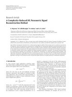
In Figure 2, the distance between the hyperplane and
f (x)is1/
w. The margin of the separating hyperplane
is defined to be 2/
w. The learning problem is hence
reformulated as minimize
w
2
= w
T
w subject to the con-
straints of linear separation as in (18). This is equivalent to
maximizing the distance of the hyperplane between the two
classes; this maximum distance is called the support vector.
The optimization is now a convex quadratic programming
problem:
Minimize

w,b
Φ
(
w
)
=
1
2
w
2
subject to y
i

w
T
x
i
+ b

≥
1, i = 1, , l.
(18)
This problem has a global optimum because Φ(w)
=
(1/2)w
2
is convex in w and the constraints are linear
in w and b. This has the advantage that parameters in a
quadratic programming (QP) affect only the training time
and not the quality of the solution. This problem is tractable,

but anomalies in internet traffic show a characteristic of
nonlinearity and are thus more difficult to classify. In order to
proceed to such nonseparable and nonlinear cases, it is useful
EURASIP Journal on Wireless Communications and Networking 7
to consider the dual problem as outlined in the following.
The Lagrange for this problem is
L
(
w, b, Λ
)
=
1
2
w
2
−
l

i=1
λ
i

y
i

w
T
x
i
+ b


−
1

, (19)
where Λ
= (λ
1
, , λ
l
)
T
are the Lagrange multipliers, one for
each data point. The solution to this quadratic programming
problem is given by maximizing L with respect to Λ
≥ 0and
minimizing with respect to w and b. Note that the Lagrange
multipliers are only nonzero when y
i
(w
T
x
i
+ b) = 1, vectors
for t his case are called support vectors since they lie closest to
the separating hyperplane. However, in case of nonseparable,
forcing zero training error will lead to poor generalization.
To take into account the fact that some data points may be
misclassified, we introduce soft margin SVM using a vector
of slack variables Ξ

= (ξ
1
, , ξ
l
)
T
that measure the amount
of violation of the following constraints:
Minimize
w,b,Ξ
Φ
(
w, b, Ξ
)
=
1
2
w
2
+ C
l

i=1
ξ
k
i
subject to y
i

w

T
φ
(
x
i
)
+ b

≥
1 − ξ
i
, ξ
i
≥ 0, i = 1, , l,
(20)
where C is a regularization parameter that controls the
tradeoff between maximizing the margin and minimizing the
training error. If C is too small, insufficient stress is placed on
fitting the training data. If C is too large, the algorithm will
overfit the dataset.
In practice, a ty pical S VM approach such as the soft
margin SVM showed excellent performance more often than
other machine learning methods [26, 33]. In case of an
intrusion detection application, supervised machine learning
approaches based on SVM were superior to intrusion
detection approaches using artificial neural networks [ 30,
33, 34]. Therefore, the high classification capability and
processing performance of soft margin SVM approach will be
useful for anomaly detection. However, because soft margin
SVM is a supervised learning approach, the labeling of the

given dataset is needed.
4.3. One-Class SVM: Unsupervised SVM. SVM algorithms
can be also adapted into an unsupervised learning algorithm
called one-class SVM, which identifies outliers amongst
positive examples and uses them as negative examples
[24]. In anomaly detection, if we consider anomalies as
outliers, one-class SVM approach can be applied to classify
anomalous packets as outliers.
Figure 3 shows the relation between a hyperplane of
one-class SVM and outliers. Suppose that a dataset has a
probability distribution P in the feature space and we want
to estimate a subset S of the feature space such that the
probability that a test point drawn from P lies outside of S
is bounded by some a priori specified value ν
∈ (0, 1). The
solution of this problem is obtained by estimating a function
Origin
Distance
Outlier
y
i
(w
T
φ(x
i
)) ≥ ρ
Figure 3: One-class SVM; the origin means the only original
member of second class.
f which is a positive function taking the value +1 in a small
region, where most of the data lies, and

−1elsewhere.
f
(
x
)
=
⎧
⎨
⎩
+1, if x ∈ S,
−1, if x ∈ S.
(21)
The main idea is that the algorithm maps the data into a
feature space H using an appropriate kernel function and
then attempts to find the hyperplane that separates the
mapped vectors from the origin with maximum margin.
Given a t raining dataset ( x
1
, y
1
), ,(x
1
, y
1
) ∈
N
×{±1},
let Φ :
N
→ H be a kernel map which transforms the

training examples into the feature space H. Then, to separate
the dataset from the origin, we need to solve the following
quadratic programming problem:
Minimize
w,b,Ξ
Φ
(
w, b, Ξ
)
=
1
2
w
2
+
1
vl
l

i=1
ξ
k
i
− ρ
subject to y
i

w
T
φ

(
x
i
)

≥
ρ − ξ
i
, ξ
i
≥ 0, i = 1, , l,
(22)
where ν is a parameter that controls the tradeoff between
maximizing the distance from the origin and containing
most of the data in the region related to the hyperplane and
corresponds to the ratio of outliers in the training set. Then
the decision function f (x)
= sgn((w · Φ(x)+b) − ρ)willbe
positive for most examples x
i
contained in the training set.
In practice, even though one-class SVM has the capability
of outlier detection, this approach is more sensitive to a
given dataset than other machine learning schemes [24, 34].
It means that deciding on an appropriate hyperplane for
classifying outliers is more difficult than in a supervised SVM
approach.
5. G-HMM Lea rning Approach
Although the above-mentioned PMAR capability is given
to SVM learning, it does not always mean the the inferred

8 EURASIP Journal on Wireless Communications and Networking
relations are reasonable. Therefore, we need to estimate more
realistic association from internet traffic. Among various
HMM learning approaches, we use G-HMM because G-
HMM has Gaussian observation outputs in continuous
probabilistic distribution. Our G-HMM approach makes a
normal behavior model to estimate hidden temporal rela-
tions of packets and evaluates anomalous behavior through
calculating ML. Moreover, G-HMM model has a possibility
of being singular when their covariance matrix is calculating.
Thus, we also need to make a better initialization when
decreasing the number of features during the G-HMM data
preprocessing.
5.1. G-HMM Feature Reduction. In G-HMM learning, a
mixture of Gaussians can be written as a weighted sum
of Gaussian densities. The observations of each state
are described by the mean value μ
i
and the covariance

i
of Gaussian density. The covariance matrix

i
is
calculated by given input sequences. When we estimate
the covariance matrix, it can often become a singular
matrix in accordance with a characteristic of the given
sequences. This is because each data value is too small
or too few points are assigned to a cluster center due

to a bad initialization of the means. In case of inter-
net traffic, this problem can also occur because each
field has too much variation. For solving this problem,
there are a variety of solutions such as constraining the
covariance to be spherical or diagonal, adjusting the prior,
or trying a better initialization using a feature reduc-
tion. Among these solutions, we apply a feature reduc-
tion for a better initialization to our G-HMM learning.
Through reducing the number of features, G-HMM has a
more stabilized initialization for preventing to be singular
matrix.
5.2. Gaussian Observation Hidden Markov Model (G-HMM).
HMM is one of the most popular means for classification
with temporal sequence data [31, 32]. It is a statistical
model with finite set of states, each of which is asso-
ciated with a probability distribution. Transitions among
the states are governed by a set of probabilities called
transition probabilities. In a particular state, an observation
can be generated, according to the associated probability
distribution. It is only the outcome not the state visible
to an external observer, and therefore states are hidden
to the outside. Formally, HMM consists of the following
parts:
(i) T
= length of the observation sequence,
(ii) N
= number of states of HMM,
(iii) M
= number of observation symbols,
(iv) Q

={q
1
, , q
n
}:states,
(v) V
={v
1
, , v
n
}: discrete set of possible symbol
observations.
If we assume that HMM model is λ,thismodelisdescribed
as λ
= (A, B, π) using the above characteristic parameters as
shown in t he following:
λ
=
(
A, B, π
)
,
A
=

a
ij

=


P

q
t
= j | q
t−1
= i

,for1≤ i, j ≤ N,
B
={b
i
(
m
)
}=

P

o
t
= m | q
t
= i

,
for 1
≤ i ≤ N,1≤ m ≤ M,
π
={π

i
}=

P

q
1
= i

,for1≤ i ≤ N,
(23)
where A is a probability distribution of state transition,
B is a probability distribution of observation symbol, and
π is a probability of initial state distribution. HMM can
be described as discrete or continuous according to the
modeling method of observable sequences. Formula (23)is
suitable to HMM with d iscrete observation events. However,
we assume that the observable sequences of internet traffic
approximate continuous distributions. A continuous HMM
has the advantages of using small input data as well as
describing Gaussian-distributed model. If our observable
sequences have Gaussian distribution, for a Gaussian pdf, the
output probability of an emitting state, x
t
= i,is
b
i
(
o
t

)
= N
⎛
⎝
o
t
, μ
i
,

i
⎞
⎠
=
1

(
2π
)
M



i


exp
⎛
⎝
−

1
2

o − μ
i


−
1

i

o − μ
i

⎞
⎠
,
(24)
where N(
·) is a Gaussian pdf with mean vector μ
i
and
covariance

i
, evaluated at o
t
. M is the dimensionality of the
observed data o. In order to make an appropriate G-HMM

model for learning and evaluating, we use known HMM
application problems in [14, 35] as follows.
Problem 1. GiventheobservationsequenceO
={o
1
, , o
T
}
and the model λ = (A, B, π), how do we efficiently compute
P(0/λ), the probability of the observation sequence given the
model.
Problem 2. Given the observation sequence O
= (o
1
, , o
T
)
and the model, how do we choose a corresponding state
sequence q
= (q
1
, , q
T
) that is optimal in some sense.
Problem 3. Given the observation sequences, how can the
HMM be trained to adjust the model parameters to increase
the probability of the observation sequences.
To determine initial HMM model parameters, we apply
the third problem using Forward-Backward algorithm [35].
Also, the first problem is related to a learning method

to find the probability in the given observation sequen-
ces. In our scheme, Maximum Likelihood (ML) applies
to the calculation of HMM learning model with Baum-
Welch method. In other words, HMM learning processes use
EURASIP Journal on Wireless Communications and Networking 9
a repetitive Baum-Welch algorithm with the g iven sequences,
and then ML is used to evaluate whether the given sequence
includes normal behavior or not.
As we mention the third problem to decide on the
parameters of an initial HMM model, we consider the
Forward variable α
t
(i) = Pr(O = O
1
O
2
, , O
t
, q
t
= S
i
|
λ). This value denotes the probability at which a partial
sequence O
={o
1
, , o
T
} is observed and the state q

i
is S
i
at time t, given the model λ. This can be solved inductively as
follows:
Forward procedure
(
1
)
Initially: α
i
(
i
)
= π
i
b
i
(
o
1
)
,for1
≤ i ≤ N;
(
2
)
For t
= 2, 3, , T, α
t


j

=
⎡
⎣
N

i=1
α
t−1
(
i
)
a
ij
⎤
⎦
b
j
(
o
t
)
,
for 1
≤ j ≤ N;
(
3
)

Finally: P
(
O
| λ
)
=
N

i=1
α
T
(
i
)
.
(25)
Similarly, we can consider the backward variable as β
t
(i) =
Pr(O = O
1
, , O
t
, q
t
= S
i
| λ):
Backward procedure
(

1
)
Initially: β
T
(
i
)
= 1, for 1 ≤ i ≤ N;
(
2
)
For t
= T − 1, ,1, β
t
(
i
)
=
N

j=1
a
ij
b
j
(
o
t+1
)
β

t+1

j

,
for 1
≤ j ≤ N;
(
3
)
Finally: P
(
O
| λ
)
=
N

i=1
πb
i
(
o
1
)
β
1
(
i
)

.
(26)
Thus, we can make initial HMM model using (25)and(26).
After deciding on init ial HMM model with Forward-
Backward algorithm, we can evaluate abnormal behavior
through calculating ML value. If we assume two different
probability functions, the value of λ can be used as our
estimator of causing a given value of o to occur. The value
is obtained by using a procedure as an ML,

λ
ML
(o). In this
procedure, we can maximize the probability of a given
sequence of observations O
={o
1
, , o
T
},giventheHMMλ
and their parameters. This probability is the total likelihood
(L
tot
) of the observations. Assume joint probability of
the observations and state sequence, for a given model
λ:
P
(
O, X
| λ

)
= P
(
O | X, λ
)
P
(
X | λ
)
= π
1
b
1
(
o
1
)
a
1
b
11
(
o
2
)
a
1
b
22
(

o
3
)
···
(27)
To get the total probability of the observations, w e sum across
all possible state sequences:
L
tot
= P
(
O | λ
)
=

x
P
(
O | X, λ
)
P
(
X | λ
)
. (28)
W hen we maximize probability Pr(O
| λ), we need to adjust
the initial HMM model parameters. However, there is no
known way to analytically solve for λ
= (A, B, π). Thus, we

determine the parameters using the Baum-Welch method
with an iterative procedure providing local maximization.
Let ξ
t
(i, j) denote the probability of being in state q
i
at time
t and in state j at time t + 1, given the model and the
observation:
ξ
t

i, j

=
P

q
t
= i, q
t+1
=
j
O, λ

=
P

q
t

= i, q
t+1
= j, O/λ

P
(
O/λ
)
=
α
t
(
i
)
a
ij
b
j
(
o
t+1
)
β
t+1

j

P
(
O/λ

)
=
α
T
(
i
)
a
ij
b
j
(
o
t+1
)
β
t+1

j


N
i
=1

N
j
=1
α
T

(
i
)
a
ij
b
j
(
o
t+1
)
β
t+1

j

.
(29)
Also, let γ
t
(i) be defined as the probability of being in
state i at time t, given the entire observation sequences and
model. This can be related to ξ
t
(i, j) by summing γ
t
(i) =

N
j

=1
ξ
t
(i, j). If we sum over the time index t,itcanbe
interpreted as the expected n umber of times that state i is
visited or expected number of transitions made from state
i. It is also the expected number of transitions from state
i to state j. Using the concept of event occur rences, we
can reestimate the parameters of new HMM, namely,
λ =
(A, B, π),
π = γ
1
(
i
)
= number o f times in state i at time t = 1,
a
ij
=

T−1
t
=1
ξ
t

i, j



T−1
t
=1
γ
t
(
i
)
=
Expected number of transitions from state i to state j
Expected number of transitions from state i
,
b
j
=

T
t
=1,o
t
=v
k
γ
t

j


T
t

=1
γ
t

j

=
Expected number of times in state j and observing symbol v
k
Expected number of times in state j
.
(30)
10 EURASIP Journal on Wireless Communications and Networking
Hence, if we assume that internet traffic sequences are
given after initial parameter setup by Forward-Backward
algorithm, updating HMM parameters in accordance with
the given sequences is the same as HMM learning to make
new model
λ = (A, B, π) and calculating a ML value about a
specific internet traffic sequence. It is a process of G-HMM
testing to derive L
tot
.
6. Experiment Datasets and Parameters
The 1999 DARPA IDS data set was collected at MIT Lincoln
Lab to evaluate intrusion detection system, which contained
a wide variety of intrusion simulated in a military network
environment [20]. The entire internet packet including
the entire payload were recorded in tcpdump [36]format
and provided for evaluation. The data consisted of three

weeks of training data and two weeks of test data. Among
these datasets, we used attack-free training data for nor-
mal behavior modeling, and attack data was used to the
construction of anomaly score in Tab l e 1.Moreover,for
additional learning procedure and anomaly modeling, we
generated a variety of anomaly attack data such as covert
channels, malformed packets, and some DoS attacks. The
simulated attacks were included in one of following five
categories, and they had DARPA attacks and generated
attacks:
(i) Denial of Service: Apache2, arppoison, Back, Cra-
shiis, DoSNuke, Land, Mailbomb, SYN Flood,
Smurf, sshprocesstable, Syslogd, tcpreset, Teardrop,
Udpstorm, ICMP flood, Teardrop attacks, Peer-to-
peer attacks, Permanent denial-of-service attacks,
Application level floods, Nuke, Distributed attack,
Reflected attack, Degradation-of-serv ice attacks, Un-
intentional denial of service, Denial-of-Service Level
II, Blind denial of service;
(ii) Scanning: insidesniffer, Ipsweep, Mscan, Nmap, que-
so, r esetscan, satan, saint;
(iii) Covert Channel: ICMP covert channel, Http covert
channel, IP ID covert channel, TCP SEQ and ACK
covert channel, DNS tunnel;
(iv) Remote Attacks: Dictionary, Ftpwrite, Guest, Imap,
Named, ncftp, netbus, netcat, Phf ppmacro, Sendmail
sshtrojan Xlock X snoop;
(v) Forged Packets: Targa3.
In this experiment, we used soft margin SVM as a gen-
eral supervised learning algorithm, one-class SVM as an

unsupervised learning algorithm, and G-HMM. In order to
make the dataset more realistic, we organiz ed many of the
attacks so that the resulting data set consisted of 1 to 1.5%
attacks and 98.5 to 99% normal objects. For soft margin
SVM, we consisted of learning dataset with above-described
dataset. This dataset had 100,000 normal packets and 1,000
to 1,500 abnormal packets for training and evaluating each.
In the case of unsupervised learning algorithms which
were one-class S VM and G-HMM, the dataset consisted of
100,000 of normal packets for training and 1,000 to 1,500
of various kinds of packets for evaluating. In other words,
in case of one-class SVM, the training dataset had only
normal traffic because they had unlabeled learning ability.
In case of G-HMM, G-HMM made a normal behavior
model using norm al data, and then G-HMM calculated the
ML values of the normal behavior model and test dataset.
Then the combined dataset with normal and abnormal is
tested.
SVM has a variety of kernel functions and their param-
eters, and we had to decide a regularization parameter, C.
The kernel function transforms a given set of vectors to
a possible higher-dimensionalspaceforlinearseparation.
For SVM learning, the value of C was 0.9 to 10, d in
a polynomial kernel was 1, σ in a radial basis kernel
was 0.0001, κ and θ in a sigmoid kernel were 0.00001
each. The SVM kernel functions that we considered were
linear, polynomial, radial basis kernels, and sigmoid as fol-
lows:
inner product: K


x, y

=
x · y,
polynomial with deg d: K

x, y

=

x
T
y +1

d
,
radial basis with width σ: K

x, y

=
exp

−


x − y


2

2σ
2

,
sigmoid with parameter κ and θ:
K

x, y

=
tanh

κx
T
y + θ

.
(31)
For G -HMM learning algorithm, input data was presented
as N
× p data matrix. N was the number of all inputs and
p was the length of each input. The number of states could
be adjusted with various numbers. In this experiment, the
default state was 2, and we used 4 and 6 states. Maximum
number of cycles of Baum-Welch was 100. In our experiment
we used the SVMlight, Libsvm, and HMM tools [37–
39].
7. Experimental Results and Analysis
In this section we detail the entire results of our proposed
approaches. To evaluate our approaches, we used three

performance indicators from intrusion detection research.
The correction rate is defined as the number of correctly
classified normal and abnormal packets divided by the total
size of the test data. The false positive rate is defined as the
total number of normal data that were incorrectly classified
as attacks divided by the total number of normal data. The
falsenegativerateis defined as the total number of attack data
that were incorrectly classified as normal trafficdividedby
the total number of attack data.
7.1. Field Selection Results. We discuss field selection using
GA. In order to find reasonable genetic parameters, we made
preliminary tests using the typical values mentioned in the
literature [11]. Table 2 describes the 4 times preliminary test
results.
EURASIP Journal on Wireless Communications and Networking 11
Table 2: Preliminary test parameters of GA.
No. of populations Reproduction rate (pr) Crossover rate (pc) Mutation rate (pm) Final fitness value
Case no.1 100 0.100 0.600 0.001 11.72
Case no.2 100 0.900 0.900 0.300 14.76
Case no.3 100 0.900 0.600 0.100 25.98
Case no.4 100 0.600 0.500 0.001 19.12
30
28
26
24
22
20
18
16
14

12
0
20 40
60
80 100 120
Generation
Weighted sum
GA feature selection using weighted polynomial equation
Best
= 11.72
Case number 1
Best = 14.76
30
28
26
24
22
20
18
16
14
12
020
40
60 80 100
120
Generation
Weighted sum
GA feature selection using weighted polynomial equation
Case number 2

Best = 25.98
30
28
26
24
22
20
18
16
14
12
0
20 40
60
80 100 120
Generation
Weighted sum
GA feature selection using weighted polynomial equation
Case number 3
Best = 19.125
30
28
26
24
22
20
18
16
14
12

020
40
60 80 100
120
Generation
Weighted sum
GA feature selection using weighted polynomial equation
Case number 4
Figure 4: Evolutionary process according to preliminary test parameters.
Figure 4 showsfourgraphsofGAfeatureselectionwith
the fitness function (10) according to Ta b l e 2 parameters. In
Case no.1 and Case no.2, the resultant graph seems to have
rapidly converging values because of too low reproduction
rate and too high crossover and mutation rate, respectively.
In Case no.3, the graph seems to be constant values because
of too high reproduction rate. Finally, the fourth graph of
Case no.4 seems to be converging with appropriate val-
ues. The d etailed results of Case no.4 are described in
Table 3.
Although we found the appropriate GA condition for
our problem domain by the preliminary tests, we tried
to optimize the best generation from total generations.
Through using c-SVM learning, we knew that the final
generation was well optimized. Generation 91–100 showed
the best correction rate and relatively fast processing time.
Moreover, as comparing generation 16–30 with generation
46–60, fewer fields do not always guarantee faster processing
because the processing time is also dependant on the value of
the fields.
12 EURASIP Journal on Wireless Communications and Networking

Table 3: GA field selection results of preliminary test no.4.
Generation units
Number of
selected fields
N umber of selected fields CR (%) FP (%) FN (%) PT (msec)
01–15 19
2, 5, 6, 7, 8, 9, 10, 11, 12, 13, 14, 15, 16, 17, 19, 21, 22, 23, 24 96.68 1.79 7.00 2.27
16–30 15
2, 5, 6, 7, 8, 9, 10, 11, 12, 16, 17, 20, 21, 23, 24 95.00 0.17 16.66 1.90
31–45 15
2, 5, 6, 7, 8, 9, 10, 11, 12, 16, 17, 20, 21, 23, 24 95.00 0.17 16.66 1.90
46–60 18
1, 2, 5, 6, 7, 8, 9, 10, 11, 12, 13, 14, 17, 19, 20, 22, 23, 24 95.12 0.00 16.66 1.84
61–75 17
2, 5, 6, 7, 8, 9, 10, 11, 12, 13, 14, 15, 16, 17, 19, 20, 21 73.17 0.00 91.60 0.30
76–90 17
2, 5, 6, 7, 8, 9, 10, 11, 12, 13, 14, 15, 16, 17, 19, 20, 21 73.17 0.00 91.60 0.30
91–100 15
3, 5, 6, 7, 9, 12, 13, 16, 17, 18, 19, 21, 22, 23, 24 97.56 0.00 8.33 1.74
∗
CR:correctionrate,FP:falsepositive,FN:falsenegative,PT:processingtime.
7.2. SVM Results. In this resultant analysis, the two SVMs
were tested as follows: soft margin SVM as a supervised
method and one-class SVM as an unsupervised method. The
results are summarized in Table 4. Each SVM approach was
tested with four kinds of different SVM kernel functions. The
high performance of soft margin SVM is not surprising since
it uses labeled knowledge. Also, four SVM kernels showed
similar performance in experiments on soft margin SVM.
In case of one-class SVM, RBF kernel provided the best

performance (94.65%). However, the false positive was high
as in our previous consideration. Moreover, we could not see
the result of sigmoid kernel experiment because the sigmoid
kernel was overfit. Moreover, in one-class SVM experiments,
the experiment results were very sensitive to choose a kernel.
In these experiments, the PMAR value of 7 and the support
rate of 0.33 were used.
7.3. One-Class SVM versus G-HMM Results. Even though the
false rates of one-class SVM is high, one-class SVM showed
the similar correction rate in comparison with soft margin
SVM, and it does not need preexisting knowledge. Thus, in
this experiment, one-class SVM with PMAR was compared
with G-HMM. The inputs of the one-class SVM were
preprocessed using PMAR with two unit sizes (5 and 7) and
minimum support rate 0.33. Moreover, G-HMM was learned
with three states (2, 4, and 6). In data preprocessing of G-
HMM, we used a feature reduction to prevent covariance
matrix from being singular matrix. Let us think about the
number of features. The total size of TCP and IP headers
is 48 bytes (384 bits) long. Each option field is assumed
to be 4 bytes long. And the smallest field of TCP and IP
header is 3 bits. So the number of features can be 128(384/3)
maximum. Our feature reduction converts two bytes into
one feature of G-HMM. If the size of a field is over two
bytes, the field is divided by each two and converted into one
feature each for G-HMM. Thus, total features can be ranged
between 128 and 20.
From results shown in Ta b l e 5, the better the perfor-
mance of the one-class SVM presented, the bigger the
PMAR size. In contrast, the smaller the number of G-

HMM states, the better the correction rate. Although G-
HMM showed better performance in estimating hidden
temporal sequences, the false alarm rate was too high. In this
comparison experiment, probabilistic sequence estimation
of G-HMM was superior to one-class SVM with PMAR
method. However, one-class SVM provided more stable
correction rate and false positive rate.
7.4. Cross-Validation Tests. Cross-validation test was per-
formed using 3-fold cross-validation method on 3,000
normal packets which were divided into 3 subsets, and the
holdout method [40] was repeated 3 times. Specifically,
we used one-class SVM with PMAR size 7 because this
scheme showed the most reasonable performance among our
proposed approaches. Each time we ran a test, one of the
3 subsets was used as the training set, and all subsets were
put together to form a test set. The results were illustrated
in Tab l e 6 and showed that our method depends on which
training set was used. In our experiments, the training with
validation set no.1 showed the best correction rate across all
of the three cross-validation tests and a low false positive
rate. In other words, the validation set no.1 for training
had well-organized normal features. Especially, validation
set no.1 for training and validation set no.3 for testing
showed the best correction rate. Even though all validation
sets were attack-free datasets from MIT Lincoln Lab, there
were many differences between validation sets. As a matter
of fact, this validation test depends closely on how well the
collected learning sets consist of a wide variety o f normal and
abnormal features.
8. Conclusion

The overall goal of our temporal relation based on machine
learning approaches is to be a general framework for
detecting and classifying novel attacks in internet traffic.
We designed four major components: the field selection
component using GA, the data preprocessing component
using PMAR and HMM reduction method, the machine
learning approaches using SVMs and G-HMM, and the
verification component using m-fold cross-validation. In
the first part, an optimized generation of field selection
with GA had relatively fast processing time and better
correction rate than the rest of the generations. In the second
part, we proposed PMAR and HMM reduction method for
data preprocessing. PMAR was used to support temporal
variation between learning inputs in SVM approaches.
EURASIP Journal on Wireless Communications and Networking 13
Table 4: The overall experiment results of SVMs.
Kernels Correction rate (%) False positive rate (%) False negative r ate (%)
Soft margin SVM
Inner product 90.13 10.55 4.36
Polynomial 91.10 5.00 10.45
RBF 98.65 2.55 11.09
Sigmoid 95.03 3.90 12.73
One-class SVM
Inner product 53.41 48.00 36.00
Polynomial 54.06 45.00 46.00
RBF 94.65 20.45 44.00
Sigmoid — — —
Table 5: The overall experiment results of one-class SVM versus G-HMM.
PMAR/states Correctionrate(%) Falsepositiverate(%) Falsenegativerate(%)
One-class SVM PMAR

5 80.10 23.76 19.20
7 94.65 20.45 44.00
G-HMM States
2 90.95 40.00 6.06
4 83.01 43.30 12.12
6 65.55 80.00 12.12
Table 6: 3-fold cross-validation results.
Training Test set
Correction
rate (%)
Average
rate (%)
Valida tion set no.1
Validation set no.1 53.0
69.37
Validation set no.2 67.1
Validation set no.3 88.0
Valida tion set no.2
Validation set no.1 37.7
49.57
Validation set no.2 52.0
Validation set no.3 59.0
Valida tion set no.3
Validation set no.1 59.3
56.7
Validation set no.2 62.9
Validation set no.3 47.9
HMM reduction method was applied to make more well-
distributed HMM sequences for preventing singular matrix
during HMM learning. In the third part, our key machine

learning approaches were proposed. One of them was to use
two different SVM approaches to provide supervised and
unsupervised learning features separately. For comparison
between SVMs, one-class SVM with an unlabeled feature
showed a correction rate similar to the soft margin SVM.
The other machine learning approach was to estimate hidden
relations in internet trafficusingG-HMM.InthecaseofG-
HMM approach, it proved to be one of the best solutions to
estimating hidden sequences between packets. However, its
false alarm was too high to allow it to be applied to real world.
In conclusion, when we considered temporal sequences of
SVM inputs with PMAR, one-class SVM approach had better
results than G-HMM approach. Moreover, our one-class
SVM experiment was verified by m-fold cross-validation.
Future work will involve trying to find a solution for
decreasing false positive rates in one-class SVM and G-
HMM, considering more realistic packet association such as
more elaborated flow generation over PMAR and G-HMM
and applying this framework to the real world over TCP/IP
traffic.
Acknowledgments
A part of SVM-related researches in this paper are orig-
inated from IEEE IAW 2005 and Information Sciences,
Volume 177, Issue 18 [41, 42]. The revised paper includes
whole new Hidden Markov Model-based approach and
the updated performance analysis, and overall parts like
abstract, introduction, and conclusion are rewritten, and
the main approach in Section 4 was also fully revised with
coherence.
References

[1] D. Anderson et al., “Detecting unusual program behavior
using the statistical component of the Next-Generation Intru-
sion D etection Expert System (NIDES),” Tech. Rep. SRI-
CSL-95-06, Computer Science Laboratory, SRI International,
Menlo Park, Calif, USA, 1995.
[2] “Expert System (NIDES),” type SRI-CSL-95-06, Computer
Science Laboratory, SRI International, Menlo Park, Calif,
USA, 1995.
[3] J. B. D. Cabrera, B. Ravichandran, and Raman K. Mehra,
“Statistical traffic m odeling for network intrusion detection,”
in Proceedings of the IEEE International Workshop on Modeling,
Analysis, and Simulation of Computer and Telecommunication
Systems, pp. 466–473, San Francisco, Calif, USA, 2000.
[4] W. Lee and D. Xiang, “Information-theoretic measures for
anomaly detection,” in Proceedings of the IEEE Symposium on
Security and Privacy, pp. 130–143, May 2001.
[5] J. Ryan, M-J. Lin, and R. Miikkulainen, “Intrusion detection
with neural networks,” in Proceedings of the Workshop on AI
Approaches to Fraud Detection and Risk Management, pp. 72–
77, AAAI Press, 1997.
14 EURASIP Journal on Wireless Communications and Networking
[6] L. Ertoz et al., “The MINDS—minnesota intrusion detection
system,” in Next Generation Data Mining, MIT Press, Cam-
bridge, Mass, USA, 2004.
[7]E.Eskin,A.Arnold,M.Prerau,L.Portnoy,andS.Stolfo,
“A geometric framework for unsupervised anomaly detection:
detecting intrusions in unlabeled data,” in Data Mining for
Security Applications, Kluwer Academic, Boston, Mass, USA,
2002.
[8] L. Portnoy, E. Eskin, and S. J. Stolfo, “Intrusion detection with

unlabeled data using clustering,” in Proceedings of the ACM
CSS Workshop on Data Mining Applied to Security (DMAS ’01),
Philadelphia, Pa, USA, November 2001.
[9] S.Staniford,J.A.Hoagland,andJ.M.McAlerney,“Practical
automated detection of stealthy portscans,” Journal of Com-
puter Security, vol. 10, no. 1-2, pp. 105–136, 2002.
[10] S. Ramaswamy, R. Rastogi, and K. Shim, “Efficient algorithms
for mining outliers from large data sets,” in Proceedings of the
ACM SIGMOD Conference.
[11] M. Mitchell, An Introduction to Genetic Algorithms, MIT Press,
Cambridge, Mass, USA, 1998.
[12] J. Yang and V. Honavar, “Feature subset selection using a
genetic algorithm,” in Proceedings of the Genetic Programming
Conference, pp. 380–385, Stanford, UK, 1997.
[13] V. Vapnik, The Nature of Statistical Learning Theory,Springer,
New York, NY, USA, 1995.
[14] Z. Ghahramani, “An introduction to hidden Markov models
and Bayesian networks,” i n Hidden Markov Models: Applica-
tions in Computer Vision, World Scientific Publishing, River
Edge, NJ, USA, 2001.
[15] K. C. Claffy, Internet Traffic Characterization,Universityof
California at San Diego, L a Jolla, Calif, USA, 1994.
[16] K. Thompson, G. J. Miller, and R. Wilder, “Wide-area internet
traffic patterns and characteristics,” IEEE Network,vol.11,no.
6, pp. 10–23, 1997.
[17] J. Holland, Adaptation in Natural and Artificial Systems,The
University of Michigan Press, Ann Arbor, Mich, USA, 1995.
[18] K. Ahsan and D. Kundur, “Practical data hiding in TCP/IP,”
in Proceedings of the Workshop on Multimedia Security at ACM
Multimedia, p. 7, French Riviera, France, 2002.

[19] C. H. Rowland, “Covert channels in the TCP/IP protocol
suite,” Tech. Rep. 5, 1997, First Monday, Peer Reviewed Journal
on the Internet.
[20] Lincoln Laboratory, MIT, “DARPA Intrusion Detection Eval-
uation,” />[21]C.L.Schuba,I.V.Krsul,M.G.Kuhn,E.H.Spafford, A.
Sundaram, and D. Zamboni, “Analysis of a denial of service
attack on TCP,” in Proceedings of the IEEE Symposium on
Security and Privacy, pp. 208–223, May 1997.
[22] CERT Coordination Center, “Denial of Serv ice Attacks,”
Carnegie Mellon University 2001, http://w ww.cert.org/tech
tips/denial of service.html.
[23] C. Cortes and V. Vapnik, “ Support-vector networks,” Machine
Learning, vol. 20, no. 3, pp. 273–297, 1995.
[24] B. Sch
¨
olkopf,J.C.Platt,J.Shawe-Taylor,A.J.Smola,andR.
C. Williamson, “Estimating the support of a high-dimensional
distribution,” Neural Computation, vol. 13, no. 7, pp. 1443–
1471, 2001.
[25] M. Pontil and A. Verri, “Properties of Support Vector
Machines,” Tech. Rep. AIM-1612, CBCL-152, Massachusetts
Institute of Technology, Cambridge, Mass, USA, 1997.
[26] T. Joachims, “Estimating the generalization performance of a
SVM efficiently,” in Proceedings of the International Conference
on Machine Learning,MorganKauffmann, 2000.
[27] H. Byun and S. W. Lee, “A survey on pattern recognition appli-
cations of support vector machines,” International Journal of
Pattern Recognition and Artificial Intelligence,vol.17,no.3,pp.
459–486, 2003.
[28] K. A. Heller, K. M. Svore, A. Keromytis, and S. J. Stolfo,

“One class support vector machines for detecting anomalous
windows registry accesses,” in Proceedings of the Workshop on
Data Mining for Computer Security, 2003.
[29] W. Hu, Y. Liao, and V. R. Vemuri, “Robust support vector
machines for anomaly detection in computer security,” in Pro-
ceedings of the International Conference on Machine Learning
(ICML ’03), Los Angeles, Calif, USA, July 2003.
[30] A. H. Sung et al., “Identifying important features for intru-
sion detection using support vector machines and neural
networks,” in Proceedings of the Symposium on Applications
and the Internet (SAINT ’03), pp. 209–217, 2003.
[31] R. Agrawal, T. Imilienski, and A. Swami, “Mining association
rules between sets of items in large databases,” in Proceedings
of the ACM SIGMOD International Conference on Management
of Database, pp. 207–216, 1993.
[32]D.W.Cheung,V.T.Ng,A.W.Fu,andY.Fu,“Efficient
mining of association rules in distributed databases,” IEEE
Transactions on Knowledge and Data Engineering,vol.8,no.
6, pp. 911–922, 1996.
[33] S. Dumais and H. Chen, “Hierarchical classification of Web
content,” in Proceedings of the 23rd annual international ACM
SIGIR Conference on Research and Development in Information
Retrieval, pp. 256–263, Athens, Greece, July 2000.
[34] B. V. Nguyen, “An Application of support vector machines to
anomaly detection,” Tech. Rep. CS681, Research in Computer
Science-Support Vector Machine, 2002.
[35] J. Bilmes, “A gentle tutorial on the EM algorithm and its
application to parameter estimation for gaussian mixture
and hidden markov models,” Tech. Rep. ICSI-TR-97-021,
International Computer Science In stitute (ICSI), Berkeley,

Calif, USA, 1997.
[36] V. Jacobson et al., “tcpdump,” June 1989, dump
.org/.
[37] T. Joachmims, “mySVM—a Support Vector Machine,” Univer-
sity Dortmund, 2002.
[38] C C. Chang, “LIBSVM : a library for support vector
machines,” 2004.
[39] Z. Ghahramani, HMM, />∼zou-
bin/software.html.
[40] C. G. Atkeson, A. W. Moore, and S. Schaal, “Locally Weighted
Learning for Control,” Artificial Intelligence Review, vol. 11, no.
1–5, pp. 75–113, 1997.
[41] T. Shon and J. Moon, “A hybrid machine learning approach
to network anomaly detection,” Information Sciences, vol. 177,
no. 18, pp. 3799–3821, 2007.
[42]T.Shon,Y.Kim,C.Lee,andJ.Moon,“Amachinelearning
framework for network anomaly detection using SVM and
GA,” in Proceedings of the 6th Annual IEEE System, Man and
Cybernetics Information Assurance Workshop (SMC ’05),pp.
176–183, June 2005.