Báo cáo hóa học: " Research Article Distributed and Collaborative Node Mobility Management for Dynamic Coverage Improvement in Hybrid Sensor Networks" doc

Hindawi Publishing Corporation
EURASIP Journal on Wireless Communications and Networking
Volume 2011, Article ID 724136, 17 pages
doi:10.1155/2011/724136
Research Ar ticle
Distributed and Collaborat ive Node Mobility Management for
Dynamic Coverage Improvement in Hybrid Sensor Networks
Thakshila Wimalajeewa
1
and Sudharman K. Jayaweera
2
1
Department of Electrical Engineering and Computer Science, Syracuse University, Syracuse, NY 13244, USA
2
Department of Electrical and Computer Engineering, University of New Mexico, Albuquerque, NM 87131, USA
Correspondence should be addressed to Thakshila Wimalajeewa,
Received 25 April 2010; Revised 15 January 2011; Accepted 4 February 2011
Academic Editor: Amiya Nayak
Copyright © 2011 T. Wimalajeewa and S. K. Jayaweera. This is an open access article distributed under the Creative Commons
Attribution License, which permits unrestricted use, distribution, and reproduction in any medium, provided the original work is
properly cited.
With recent advances in deploying sensor nodes mounted on mobile platforms, node mobility is becoming an attractive alternative
to improve network coverage dynamically in sensor networks. However, due to energy constraints, it may not be cost effective to
deploy a large number of mobile nodes for continuous movements. It might be more desirable to allow only a certain number of
nodes to be mobile depending on the affordable cost a nd desired performance levels. This paper proposes an efficient distributed
mobility protocol for mobile node navigation in a hybrid sensor network consisting of both static and mobile nodes to provide
efficient time-varying coverage after the initial deployment. In the proposed s cheme, mobile nodes collaborate with neighboring
static nodes to find their candidate locations to move at each movement step in order to maximize the coverage time of the area not
covered by static nodes. We also develop an efficient sequential algorithm to find the exposure in a hybrid network, which reflects
the best path for a target to traverse the sensing region without being detected. By simulations, we show the effective ness of the
proposed mobility protocol in terms of the presence probability matrix and coverage time and show its suitability at the worst-case

target exposure.
1. Introduction
Mobile sensor nodes are deployed in wireless sensor net-
works in certain applications to enhance the network per-
formance dynamically. Use of node mobility to reposition
sensors at the deployment stage to provide a uniform cov-
erage was considered in [1–5], based on different techniques.
However, these studies do not consider how to exploit the
node mobility in possible performance improvement after
the initial deployment stage. Liu et al. in [6] showed that
the coverage can be improved dynamically by allowing nodes
to be mobile continuously in a mobile sensor network over
time unlike in a static network. Distributed detection and
tracking tasks by mobile sensor networks consisting only
mobile nodes were addressed by some recent work. In [7], the
problem of target detection using a mobile sensor network is
addressed where the authors analyzed the detection latency.
In [8], algorithms to find upper and lower bounds for the
target exposure, which is defined as the target traversal which
resultsintheworst-casedetectionperformance,inamobile
sensor network deployed for mobile target detection were
proposed. In [9], a cat-and-mouse game between targets and
mobile nodes was presented based on the sensing capabilities
of targets and mobile nodes where mobile nodes try to detect
the target as quickly as possible when the target is tr ying
to evade the network before being detected. In [10, 11],
distributed tracking by mobile sensor networks is addressed.
However, deploying a large number of mobile sensor
nodes is not as cost effective as deploying static nodes in
a sensor network due to energy constraints. Thus, it is

desirable to allow only a fraction of total nodes to be
mobile to improve the network performance depending on
application requirements. Use of hybrid sensor networks
consisting of both static and mobile nodes is becoming
attractive in current sensor network applications. These
hybrid networks provide a better tradeoff between the cost
of mobile node deployment and the required performance
levels. In [12, 13], algorithms for reposition of mobile nodes
2 EURASIP Journal on Wireless Communications and Networking
at the initial deployment stage are developed in hybrid sensor
networks. In [12], mobile nodes are directed to move towards
the coverage holes detected by static nodes to improve the
coverage. In [13], impact of the node density to provide k-
coverage at the deployment stage in a hybrid sensor network
is discussed. In these approaches, it was assumed that the
mobile nodes move only once during the deployment stage
and remain stationary while the sensor network performs
specific operations. In [14], mobile node navigation towards
a specific goal in a hybrid sensor network is addressed where
static nodes are used to guide the mobile nodes. Distributed
detection by hybrid sensor networks is also addressed in
recent works [15, 16] when the sensor node and target
positions are known. Target tracking performance of an
integrated mobile-static sensor network is addressed in [17]
where t he mobile nodes are used to aid the data propagation
when the communication ranges of static nodes are limited.
However, neither of the above works addressed the problem
of how to efficiently cover the uncovered area by static nodes
in a hybrid sensor network dynamically, by node mobility
over time to provide an efficient time-varying coverage.

2. Motivation, Contribution,
and Organization
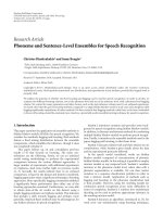
Consider a hybrid sensor network deployed in a square
region as shown in Figure 1, where the union of checked
circles represents the area covered by static nodes while the
union of solid circles represents the area covered by mobile
nodes, respectively. When t he nodes are first deployed in
a region, a random placement is often desirable especially
when aprioriknowledge of the terrain is unavailable.
However, such random deployment strategies may not result
in effective coverage always, since some nodes might be
overly clustered while some of them might be sparsely
located. Use of node mobility to reconfigure the node
locations to improve the coverage of such networks was
addressed by some authors, for example, in [1, 2, 12]. In these
approaches, nodes move only during the deployment stage
and the maximum coverage area achieved by the network
after reconfiguration is limited by the number of total nodes
and nodes’ sensing ranges. For example, if the total number
of nodes is relatively small, even by reconfiguration of mobile
nodes to provide a uniform coverage, a large portion of the
network may remain not covered. On the other hand, node
failures after the initial reconfiguration might cause coverage
holes in the network. Thus, the problem addressed in this
paper is how to effectively use the node mobility of mobile
nodes to provide an efficient dynamic coverage of the region
of interest after the initial deployment stage.
Exploiting mobile nodes for continuous coverage in
mobile sensor networks is addressed by [6] when the
nodes perform random and independent mobility. Although

random mobility models are desirable in many applications,
and they need minimum coordinations among nodes, they
may not always be ideal for hybrid networks consisting of
both static and mobile nodes. We need to consider the
following factors in d esigning an algorithm for mobile node
Figure 1: Hybrid sensor network consisting of both static and
mobile nodes: solid circles-mobile nodes and checked circles-static
nodes.
navigation in a hybrid sensor network to provide efficient
dynamic coverage.
(i) In a hybrid sensor network, a certain portion of the
field is covered always (as shown by the union of checked
circles in Figure 1) as mentioned before. Mobile nodes are
required to assist providing the cov erage for the area that is
not covered by static nodes. If a random and independent
mobility scheme is used, there might be overlappings of the
sensing ranges of mobile and static nodes since there is no
coordination among nodes. In many real world applications,
a mobile node (a sensor node mounted on a mobile
platform,) has a fixed power cost for the mobility. Even
though sensor nodes mounted on mobile platforms can carry
more battery supplies to move a considerable amount of
time/distance continuously, it is important to ensure that the
available energy is effectively used to perform the required
surveillance task, that is, to provide an effective time-varying
coverage in the d esired field in a given duration of time.
Thus, it is required to use mobile nodes to cover only the
areas uncovered by static nodes minimizing the overlapping
between the mobile and static nodes’ sensing r anges.
(ii) When nodes are mobile, previously covered areas

by mobile nodes become uncovered while uncovered areas
become covered. This requires to manage the mobility of
the mobile nodes such that to minimize the duration that a
particular location is uncovered. Random mobility schemes
do not address these issues.
(iii) If the network does not have any prior knowledge
about the sensing field, it is desired that any point not covered
by the static nodes is covered almost equally to maintain an
approximately uniform coverage over time.
Taking these factors into account, in this paper, we
propose a new distributed mobility protocol for mobile node
navigation in a hybrid sensor network. In the proposed
EURASIP Journal on Wireless Communications and Networking 3
scheme, collaborating with static nodes, mobile nodes pro-
vide an efficient dynamic coverage in the area not covered by
the static nodes. More specifically, we assume that the sensor
network is partitioned into square cells such that a node can
cover such a cell completely when it is located at the center of
the cell. We divide these cells into two categories: static and
void cells. Static cells correspond to the cells in which there
is at least one static node, and the void cells are the ones in
which there is no any static node. M obile nodes are directed
to move among these void cells based on a certain criteria.
Each of such void ce lls i s given a certain base price.Thisbase
price is updated by static nodes based on the time that the
void cell remains not covered by at least one mobile node. At
each movement step, mobile nodes communicate with their
closest static nodes locally to search for void cells which are
not covered for a long time. Static nodes provide necessary
information for mobile nodes in their neighborhoods. At

a given time, we assume that a mobile node can visit a
certain number of candidate void cells from its c urrent
position. These candidate void cells are determined by the
mobile node’s maximum speed. Taking base prices ( collected
from neig hboring static nodes) of the candidate void cells
into account, each mo bile node selects the best void cell to
be visited by the next time step. In the proposed scheme,
since the node mobility is performed by mobile nodes by
collaborating w ith static nodes, we call the proposed scheme
“mobile-static collaborative mobility model.” In simulations,
we show the effectiveness of the mobile-static collaborative
mobility model in terms of the presence probability matrix
and the average time that an a rbitrary point in the network
is not covered. (The presence probability matrix contains the
probabilities of the presence of at least one node at each cell
at any given time instant.)
We furt her analyze the e ffectiveness of the proposed
mobility scheme in terms of the worst-case detection perfor-
mance when the network is deployed for detection applica-
tions. It is noted that when the application r equirement is
different, there are other performance measures that can be
selected (depending on the type of application) to e valuate
the effectiveness of the proposed mobility model. However,
in the paper, we restrict ourselves only to a target detection
application which is one of the fundamental tasks performed
by a sensor network. We analyze the worst-case detection
performance in terms of the exposure [8, 18, 19], which
reflects the quality of the sensor network when the target
tries to evade the network with minimum probability of
being detected. To find the exposure, we develop an efficient

sequential methodology based on the presence probability
matrix. The proposed methodology to find the exposure is
valid for hybrid sensor networks with arbitrary mobility
models as far as the knowledge of the presence probability
matrix is available. We show that the proposed mobility
scheme results in a sig nificant performance improv ement at
theworst-casetargetexposure compared to that with random
mobility schemes especially when the fraction of mobile
nodes in the hybrid network is small.
The paper is organized as follows: Section 3
presents
the network model and the assumptions. In Section 4,
the proposed mobile-static collaborative mobility model is
described i n detail. The worst-case performance on target
detection by the hybrid sensor network with proposed
mobility protocol is addressed in Section 5.Performance
results are shown in Section 6, while the concluding remarks
are given in Section 7.
3. Network Model and Assumptions
We consider a hybrid sensor network made of N number
of sensor nodes deployed in a region R with network
dimension of b
× b.OutofN, that there are N
s
number of
static nodes and N
m
number of mobile nodes. Denote λ =
N/b
2

to be the spatial density of the nodes and λ
m
= N
m
/N
and λ
s
= N
s
/N to be the fractions of mobile and static nodes,
respectively. Let V, V
m
,andV
s
be the sets containing all
mobile and static node indices, respectively.
Suppose that the sensing region is divided into a virtual
square grid with grid length of l
=
√
2r where r is the effective
sensing radius of a sensor. We assume that both static and
mobile nodes have the same sensing radii. When a sensor
node is located at the center of a cell in the grid, the cell
is completely covered by the corresponding sensor node.
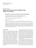
Consider the hybrid network with only static nodes as shown
in Figure 2 (droppingthemobilenodesinFigure 1). We
denote the cells that are not covered by the static nodes as
void cells (with void squares as shown in Figure 2). When
a static node is located in a particular cell (crossed cell in

Figure 2), we consider that the corresponding cell is covered
by the relevant static node and call it a static cell. However,
note that since a static node is not necessarily located at the
middle of a cell, corresponding cell may not be completely
covered by corresponding the static node. We address this
problem later and for the moment assume that the cell is
covered by the corresponding static node. Now, the problem
is how to use the mobile nodes efficiently to cover the void
cells as shown in Figure 2 over time, such that the revisiting
time of any cell by at least one mobile node is maximized.
In the following, we propose a new distributed interactive
protocol, called mobile-static collaborative mobility model to
achieve the required task by collaboration among mobile and
static nodes.
In the following, we list the specific assumptions made in
the proposed mobility algor ithm.
Assumptions. (1) All nodes have the same sensing radius.
(2) There is a fraction λ
m
of mobile nodes having enough
locomotion energy to provide dynamic coverage in a time
duration of

T where

T is determined by several factors,
such as the maximum distance that a mobile node can move
before the energ y is depleted, and application requirements.
This assumption is realistic for relatively large


T since sensor
nodes mounted on mobile platforms can carry more battery
supplies.
(3) λ
m
remains constant during the time interval

T.
(4) We consider an obstacle-free environment.
(5) Static sensor network is assumed to be connected
within the time duration

T.
4 EURASIP Journal on Wireless Communications and Networking
Figure 2: Sensor network with only static nodes.
For applications where these assumptions are not satisfied,
possible modifications to the algorithm are discussed at the
end of the Section 4.
4. Distributed Mobility Protocol
In this section, the proposed mobile-static collaborative mo-
bility model is discussed in detail.
4.1. Description of the Algorithm. Once identifying the st atic
and void cells,weassignabasepriceforeachvoid cell
according to the following rule. Initially, at time t
= 0, we
assign a base price P
= 0foreachvoid cell in which there
is at least one mobile node. For all the other void cells, we
assign P
= K where K is a large value. Let T

m
be the time
step in which the mobility management is performed, which
can be determined as given below.
4.1.1. Determining T
m
. We assume that any mobile node can
reach L
c
= 8 number of closest distinct cell centers (and
itself) as shown in Figure 3 at any given time step. Then
the maximum distant that a node has to move during time
T
m
is 2r. Thus, it is desirable to choose t he time step T
m
as
T
m
=(2r/v
max
)+s where  is a bias factor which accounts
for the scenarios when it is needed to heal the lack of coverage
at static cells which will be explained in Section 4.4 in detail.
At each time step T
m
,thebasepriceofeachvoid cell
is updated considering the time it remains uncovered (or
unvisited by at least one mobile node). More specifically, at
each step T

m
, if a particular cell is visited by a mobile node, its
base price P issettozeroandthebasepricesofallothervoid
cells are increased by 1 unit. Without loss of generality, we
assume that at time t
= 0 each mobile node has moved to the
cell center which it belongs to, and at each step T
m
,mobile
nodes move among cell centers. In the following, we explain
how a mobile node selects the best cell to be visited at each
time step distributively by collaborating with static nodes.
Current location at time t
Candidate locations at time t + T
m
2r
√
2r
Figure 3: A mobile node’s candidate locations at a given time.
Let each cell (cell center) i n the square grid be given an
ID labeled by indices 1, 2, , L
T
where L
T
≈ b
2
/l
2
is the total
number of cells. Let there be L

s
number of cells covered by
static nodes (static cells) and L
v
= L
T
− L
s
number of cells
that are not covered by static nodes (void cells). Also denote
U, U
s
,andU
v
to be the sets containing all cell indices of the
network, static cell indices and void cell indices, respectively.
4.1.2. Assigning Void Cells for Each Static Node. We assign
a certain number of void cells to each static node in the
network. Each static node in the network is responsible
for updating the base price of each void cell that belongs
to it. Corresponding void cells for each static node are
assigned based on Voronoi partitions (as shown in Figure 4).
According to Voronoi partitions, any point inside a Voronoi
polygon of a static node is closer to that static node rather
than to any other static node in the network. Thus, for a
given static node s
k
, the cell centers belonging to its Voronoi
polygon are closer to the static node s
k

than any other st atic
node in the network. We assume that each static node has the
knowledge of t he positions of the void cell centers belonging
to itself. At the initial stage, static n odes can communicate
with their Voronoi neighbors locally to construct Voronoi
polygons. It is noted that each static node needs to know
only the existence of its Voronoi neighbors and communicate
among them locally to construct the Voronoi polygon. By
knowing its own location, and based on the grid length (in
terms of the sensing range), each static node can determine
the void cells in its Voronoi polygon. Since we assume that
the static nodes are connected during the time

T in which
the node mobility is performed, the void cells belong to each
static node’s Voronoi polygon are always taken care of at each
EURASIP Journal on Wireless Communications and Networking 5
−100 −80 −60 −40 −20 0 20 40 60 80 100
−100
−80
−60
−40
−20
0
20
40
60
80
100
Y

X
Figure 4: Voronoi polygons for each static node: Solid square-static
node locations, solid circles-grid points (centers) corresponding to
static nodes and void circles-grid points (centers) corresponding to
grids not covered by static nodes.
time step. In the proposed algorithm, it is assumed that an y
void cell inside a Voronoi polygon can communicate with at
least the corresponding static node of that Voronoi polygon.
Since any mobile node is assumed to be located in a void cell,
and each void cell is assumed to belong to a Voronoi polygon
of a particular static node, it is assumed that each mobile
node can communicate at least with the corresponding static
node in that Voronoi polygon.
Denote U
s
k
to be the set of void cell indices belonging
to the Voronoi polygon of the static node s
k
for s
k
∈ V
s
and L
s
k
=|U
s
k
| be the number of void cells (cell centers)

belongs to static node s
k
.NotethatwehavethenU
v
=

k∈V
s
U
s
k
. Further denote g
s
k
(nT
m
)tobeanL
s
k
-length
vector containing the base prices for all void cells attached
to the static node s
k
at time nT
m
for s
k
∈ V
s
. Each static

node s
k
is responsible for updating g
s
k
(nT
m
)ateachtimestep
t
= nT
m
for n = 1, 2,
4.2. Updating g
s
k
(nT
m
)
4.2.1. At Time t
= 0. At time t = 0, each mobile node
broadcasts its current location (or equivalently current cell
ID) to its neighborhood, such that static nodes located close
to the corresponding mobile node receive this information. If
the corresponding mobile node’s cell ID belongs to U
s
k
,then
the static node s
k
sets the base price for the corresponding

cell to zero. Base prices for all the other cells in U
s
k
are set
to a large integer n umber K.Notethatattimet
= 0, all void
cells which have no mobile node at time t
= 0havethesame
base price K.
4.2.2. At time t
= nT
m
, n ≥ 1. At time t = nT
m
,each
mobile node broadcasts its location information (current
cell ID) to its nearest static nodes. Let N
m,k
(nT
m
)bethe
number of mobile nodes that the static node s
k
receives
location information at time nT
m
and U
m,k
(nT
m

)bethe
set corresponding to those locations (cell indices). Then
for a given static node s
k
for all cell indices c
j
∈ U
s
k
,it
checks whether c
j
also belongs to U
m,k
(nT
m
). If c
j
∈ U
s
k
∩
U
m,k
(nT
m
), the static node s
k
sets the base price of the cell c
j

to be zero. Otherwise, it increases the base price of the cell c
j
by 1 u nit.
After updating the base price vector g
s
k
(nT
m
)attimenT
m
at each static node s
k
, the problem is to determine the next
cell ID to be visited by each mobile node by time t
= (n +
1)T
m
, such that the cell-revisiting time is maximized. Denote
C
m, j
(nT
m
) to be the set of candidate locations (cells) of the
jth mobile node at time nT
m
.AlsoletU
m
j
s
k

(nT
m
)bethesetof
cell indices belonging to both C
m, j
(nT
m
)andU
s
k
.Notethat
the maximum size of the set U
m
j
s
k
(nT
m
)is|U
m
j
s
k
(nT
m
)|
max
=
L
c

+1 = 9, since we assume that each mobile node can
move to one of the 8 distinct candidat e locations and itself
during a given time step. For a given mobile node m
j
from
which the static node s
k
receives the location information,
the static node s
k
checks whether any cell in m
j
th candidate
set C
m, j
(nT
m
) belongs to U
s
k
at time t = nT
m
. If not, static
node s
k
does not need to communicate with mobile node m
j
at time nT
m
.

If any cell in m
j
th candidate set C
m, j
(nT
m
)belongsto
U
s
k
, or in other words, if the set U
m
j
s
k
(nT
m
)isnotempty,the
communication between the static node s
k
and the mobile
node m
j
is performed as follows.
(i) Based on the information received by closest mobile
nodes, the static node s
k
determines whether there are more
than two mobile nodes located within a distance d
t

.We
say the mobile node m
j
is isolated with respect to another
mobile node, if there is no at le ast one mobile node within
adistanced
t
from its current location where d
t
(equals to
4r) is a threshold distance which is determined such that
no duplicate covering occurs as discussed in Section 4.3.If
themobilenodem
j
is not isolated with respect to another
mobile node, there is a possibility for a duplicate covering;
that is, two or more mobile nodes try to cover the same cell
at the time (n +1)T
m
. Note that in the rest of the paper a
mobile node is isolated means that the mobile node is isolated
with respect to another mobile node. It is noted that (as one
reviewer pointed out), if the duplicate covering is going to
happen, the same static node is responsible for updating the
base price of the corresponding cell (the cell that both mobile
nodes are going to cover). Thus, if the static node s
k
identifies
that there are more mobile nodes within a distance of d
t

to each other, it transmits all the base prices corresponding
to the candidate locations in the set U
m
j
s
k
(nT
m
) to assist
in resolving the duplicate covering problem as discussed in
Section 4.3.Inthiscase,themobilenodem
j
selects the
best cell to be moved by time (n +1)T
m
after checking the
need for duplicate covering by locally communicating with
neighboring mobile nodes. This scenario is further discussed
in Section 4.3.
(ii) If m
j
is isolated (that is there is no any other mobile
node within a distance of d
t
from the current location of m
j
),
static node s
k
finds the cell from the set U

m
j
s
k
(nT
m
) which has
the maximum base price and sends a message corresponding
6 EURASIP Journal on Wireless Communications and Networking
tothecellIDandthemaximumcorrespondingbaseprice.
Note that all t he candidate cells for mobile node m
j
may not
belong to a one static node. In particular, they may belong
to multiple nearby static nodes. Once the mobile node m
j
gets maximum base prices from multiple static nodes which
its candidate cells belong to, it selects the best location for
time (n +1)T
m
by comparing the base prices it gets from
different static nodes and selects the one with maximum base
price. Note that if there are two or more candidate cells with
the same highest base price for a mobile node, it selects the
candidate cell randomly from those.
It is worth mentioning that if the mobile node m
j
is
isolated,thestaticnodes
k

sends only one base price and cell
ID to the mobile node m
j
(which is corresponding to the
maximum base price in the set U
m
j
s
k
(nT
m
)). On the other
hand, if m
j
is not isolated,thestaticnodes
k
has to send all
base prices and cell IDs in the set U
m
j
s
k
(nT
m
)(whichhas9
cells in the worst case).
4.3. Duplicate Covering at a Given Time. As mentioned
before, when two mobile nodes are close to each other,
there might be situations where both will try to select the
same void cell as the candidate location based on the values

of corresponding base prices. For example, consider the
scenario as depicted in Figure 5. Assume that two mobile
nodes m
1
and m
2
are located in cells represented by A and
B at time t
= nT
m
as shown in Figure 5. A ccor ding to the
information received from closest static nodes, both mobile
nodes can access to the base prices of all of their candidate
cells, marked at the north-east corner of each candidate cell
for both mobile nodes. According to the base prices, both
mobile nodes will try to select the cell C as the next location
for time (n +1)T
m
which has the highest base price from
each mobile nodes’ c andidate sets. It can be shown that this
phenomenon might happen only when two mobile nodes are
located within a maximum distance of d
t
= 2
√
2l = 4r.
Since this will lead to inefficient coverage, we propose
for two mobile nodes to exchange their information locally
to avoid duplicate covering. Since this phenomenon occurs
when two mobile nodes are located close to each other,

we assume that these two mobile nodes can exchange their
information to check whether a duplicate covering is going to
happen. I f so, they exchange the next maximum b ase prices
from their candidate sets and check which mobile node has
the second maximum base price (Note that when a mobile
node is not isolated, they have the access for base prices
of all candidate cells as discussed above). Accordingly, the
node with the second highest maximum base price selects
the corresponding cell as the candidate cell. According to
Figure 5, since the mobile node m
1
has the second maximum
base price (compared to mobile node m
2
), it moves to the
corresponding cell (denoted by cell D) while the mobile node
m
2
moves to the cell C. If the second maximum base price is
the same for both nodes, they can select either one of the
nodes to move to the cell with the second maximum base
price arbitrarily. When there are more than 1 mobile sensor
within the distance d
t
from node m
j
, the same procedure can
be extended by e xchanging the relevant information among
m
1

1
05
5
3
1
5
9
4
10
8
12
0
7
1
9
m
2
2
A
B
C
D
Candidate cells for mobile node m
1
Candidate cells for mobile node m
2
Figure 5: Duplicate covering at a given time.
those nodes. In such cases, it might be necessary to exchange
2nd, 3rd, highest base prices among neighboring mobile
nodes.

4.4. Compensating for the Lack of Coverage in a Static Cell. As
mentioned earlier in this section, since a static node may not
necessarily be located a t the ce nter of a static cell in the grid,
there are certain uncovered portions of the corresponding
cell. Note that this uncovered portion is maximized when
a static node is located very close to one of the cell corners
which it belongs to. Consider the scenario that the static node
is located very close to the north-east corner of the cell it
belongs to (denoted by c
1
), as shown in Figure 6 with a circle
with solid line. To compensate for the lack of coverage in the
corresponding cell, we propose the following procedure. It
can be shown that with the relationship between the side
length of a cell in the grid and the sensing range, when a
mobile node comes to a cell located either to the left or to the
bottom of the static cell, and if they are moved a distance of
r
− (r/
√
2) (at the worst case) beyond the cell center towards
the static cell, the uncovered portion of the corresponding
static cell can be completely covered. This is illustrated in
Figure 6 where a mobile node comes to either cell center A
or C, and if it is allo wed to move a distance of r
− (r/
√
2)
(i.e., either to B or D, resp.), the uncovered portion of the
static cell can be completely covered. To address this problem,

at time nT
m
, when a mobile node selects its candidate cell
for time (n +1)T
m
,italsocheckswhetherthereisastatic
node located to the right, left, up, or down to the selected
cell. Based on the static node location, it approximates the
required distance it should move (maximum of r
− (r/
√
2))
EURASIP Journal on Wireless Communications and Networking 7
l =
√
2r
√
2r − r
r −
r
√
2r
r −
r
√
2r
r
c
1
c

2
A
B
r
√
2
D
C
c
3
E
F
2r
∼
2.21
6
8r
Figure 6: Compensating for the lack of coverage in static cells.
beyond the selected cell center to compensate for the lack of
coverage of the static cell.
Note that according to the proposed mobility algorithm
we allow mobile nodes to move between cell centers at
consecutive time steps T
m
. However, when we need to
address this static cell compensating problem, mobile nodes
have to move little far away from a cell center. When this
happens (i.e., a mobile node may move to location B (or
D)insteadofA (or C)inFigure 6), the mobile node may
need to move a maximum distance of

≈ 2.2168r to reach i ts
next candidate cell at next time step. As shown in Figure 6,
when the mobile node is at the point D in the cell c
3
,it
can reach all candidate cells by next time step, except E
and F, by m oving a maximum distance of 2r.Toreachthe
candidate cells E and F it has to move a maximum distance
of
≈ 2.2168r. Thus, when determining the time step T
m
as
pointed out in Section 4.1.1, we need to take this scenario
into account. Thus, T
m
is selected as T
m
=(2r/v
max
)+s
where
 = 0.2168r/v
max
.
The proposed mobile-static collaborative mobility model
for node mobility management of hybrid sensor network is
summarized in Algorithm 1.
It is worth mentioning that the Algorithm 1 requires
proper time synchronization for its operation. It is assumed
that each static node enters the initialization phase by locally

communicating among them. This initial synchronization
among sensors can be a chieved with a similar scheme as
presented in [20]. During the initialization period,
(i) all static nodes broadcast their location information
locally to construct Voronoi polygon at each static
node and to assign the corresponding void cells to
each static node;
(ii) all static nodes initialize their base price ve ctors;
(iii) static nodes broadcast a message to mobile nodes in
their neighborhoods to set the timers of mobile nodes
to the initialization phase and ask to broadcast their
location information locally.
After the initialization phase, it is assumed that static and
mobile nodes manage to have time synchronization at each
time step T
m
via local communication among static and
mobile nodes. During each time step T
m
, each static and
mobile node can enter the different phases on their task
schedules as described in Algorithm 1.
4.5. Modifications to the Algorithm When Certain Assumptions
Are Relaxed. It should be noted that the algorithm is based
on certain assumptions stated in Section 3.Inthefollowing,
we discuss how the algorithm can be modified when some of
these assumptions are relaxed.
In the algorithm, it was assumed homogeneous sensors;
that is, each node has identical effective sensing radius.
According to the proposed algorithm, the nature of the

sensing radius of nodes matters when the grid length of the
virtual grid is selected. With homogeneous sensing radius,
the grid length is selected as
√
2r, since then when a sensor
node lies at the center of a cell, that cell is completely covered
by the corresponding node. If nodes have different sensing
radii, the algorithm can be modified in following ways. Let
r
max
and r
min
be the maximum and minimum values of
sensing radii of nodes.
(i) If r
max
− r
min
is small: in this case, a simple mod-
ification can be employed to the current algorithm. The
virtual grid can be constructed such that the grid length
equals to
√
2r
min
. This ensures that if any node is located
at the middle of a cell, the corresponding cell is completely
covered. If the grid length is selected as
√
2r

min
,itisnoted
that when r>r
min
, a certain portions of neighboring cells
will also be covered by the corresponding node. However,
if the difference r
max
− r
min
is small, selecting grid length as
√
2r
min
does not cause a large performance degradation with
the proposed algorithm.
(ii) If r
max
 r
min
:ifr
max
 r
min
, letting grid length
√
2r
min
and continuing moving among candidate locations
at each time step as discussed in the current algorithm would

not give effective coverage, since then many overlapping
among sensing ranges at consecutive time steps will occur for
nodes having r>r
min
. Thus, depending on the sensing radius
and allowable maximum speed, the candidate locations and
thus the time step for a movement for a given mobile node
should be carefully decided.
In the proposed algorithm, it was assumed that the
mobile nodes have enough energy to perform mobility in the
required time duration

T. As one of the reviewers pointed
out, in many real-world settings, mobile nodes have limited
energy and may deplete the power supplies before the
required task is done. In the following, we discuss how to
modify the algorithm in order to address this p roblem.
Approach 1. Assume that the energy of some mobile nodes
may be depleted before completing the required mobility
during the time interval

T.Letρ
m
j
,max
be the maximum
8 EURASIP Journal on Wireless Communications and Networking
A. NOTATIONS:
g
s

k
(nT
m
): base price vector at static node s
k
at time t = nT
m
U
s
k
:setofallvoid cell i ndices belongs to static node s
k
N
m,k
(nT
m
): number of mobile nodes from which the static no de s
k
receives locations information at time nT
m
C
m,j
(nT
m
): set of cell indices corresponding to candidate cells of mobile node m
j
at time nT
m
U
m

j
s
k
(nT
m
): set of cell indices belongs to both C
m,j
(nT
m
)andU
s
k
g
m
j
s
k
(nT
m
): base price vector corresponding to cell indices in U
m
j
s
k
P
∗
j,k
: element w ith maximum value (maximum base price) in g
m
j

s
k
(nT
m
)
c
∗
j,k
: cell index corresponding to P
∗
j,k
B. INITIALIZATION AT TIME t = 0:
Determine U
s
k
for a ll s
k
∈ V
s
based on Voronoi partitions
Initialize g
s
k
(0) as in Section 4.2.1
C. AT STATIC NO DE s
k
AT TIM E t = nT
m
:
After r eceiving location (cell) information from neighboring mobile nodes:

U pdat e the base price v e ctor g
s
k
(nT
m
)asinSection 4.2.2
for j
= 1:N
m,k
(nT
m
) do
Check
→ U
m
j
s
k
(nT
m
)isnon-empty
if U
m
j
s
k
(nT
m
)isnon-emptythen
check

→ m
j
is isolated
if m
j
is isolated then
Find P
∗
j,k
and c
∗
j,k
and transmit to mobile node m
j
else {m
j
is not isolated}
Send cell IDs and their base prices in the set U
m
j
s
k
(nT
m
) to mobile node m
j
end if
else
{U
m

j
s
k
(nT
m
)isempty}
Send nothing to m obile node m
j
end if
end for
D. A T MOBILE NODE m
j
AT TIM E t = nT
m
:
Broadcast location information to neighboring static nodes
After receiving base prices for relevant candidate locations from neighboring static nodes:
check
→ m
j
is isolated
if m
j
is isolated then
select candidate cell with maximum base price
else
{m
j
is not isolated}
call duplicate covering(m

j
)
end if
After selecting candidate cell corresponding to time (n +1)T
m
:
Check
→ need for static ce ll compensation
if static ce ll compensation is required then
Adjust the location to be moved in the selected candidate cell according to Section 4.4
else
{static cell compensation is not required}
Move to the center of the selected candidate cell by time (n +1)T
m
end if
duplicate
covering(m
j
)
Exchange local information with neighboring mobile nodes to check for duplicate covering
if yes:(duplicate covering) then
Exchange next highest base prices to det ermine the best candidate cell as in Section 4.3
else
{no:(no duplicate covering)}
select candidate cell with maximum base price
end if
Algorithm 1: Mobile-static collaborative mobility protocol.
distance that the mobile node m
j
can travel before recharg-

ing/replacing its battery. Let E
(n+1)T
m
(c
m
j
(nT
m
), c
m
j
((n +
1)T
m
)) be the energy consumption of the mobile node m
j
when moving from the cell c
m
j
(nT
m
)tothecellc
m
j
((n +
1)T
m
) during the time step from nT
m
to (n +1)T

m
where
c
m
j
(nT
m
) is the index of the cell in which the mobile node
m
j
is located at time nT
m
.Ifweassumethatasimpleenergy
model, where the energy is linearly related to the distance
EURASIP Journal on Wireless Communications and Networking 9
traveled by the mobile node, we have E
(n+1)T
m
(c
m
j
(nT
m
),
c
m
j
((n +1)T
m
)) = α

0
d(c
m
j
(nT
m
), c
m
j
((n +1)T
m
)) where
d(c
m
j
(nT
m
), c
m
j
((n+1)T
m
))is the Euclidian distance from
the location of the cell c
m
j
(nT
m
)tothecellc
m

j
((n +1)T
m
)
and α
0
is a constant (in units Joules per meter). Further let
ρ
m
j
((n+1)T
m
) = ρ
m
j
(nT
m
)+d(c
m
j
(nT
m
), c
m
j
((n+1)T
m
))
be the total distance that the mobile node m
j

has moved by
time (n +1)T
m
. We assume that each mo bile node m
j
can
update ρ
m
j
((n)T
m
)attimenT
m
by itself.
Now , as described in Section 4.1, when the mobile m
j
broadcasts its c urrent cell ID at time nT
m
,italsosendsa
message to its nearby static nodes to inform that its energy
is about to be depleted if ρ
m
j
,max
− ρ
m
j
(nT
m
) <ρ

0
where
ρ
0
is a threshold value. This value can be determined by the
average time it takes for the network to insert another mobile
node before the energy of m
j
is completely depleted. This
information lets the nearby static nodes know that the energy
of mobile node m
j
is about to be depleted, so the network
can take necessary actions to replace it. Once a new mobile
node is added to the network (this can be initially located
in a different cell), the cell in which the mobile node m
j
is
located is considered as a general void cell (in which t here is
no mobile node) and its base price is updated as described in
Section 4.2.
Note that in this approach, it is able to maintain the same
fraction of mobile nodes until the required task is completed
(time

T is elapsed). Also the mobile nodes in which the
energy is depleted can be made available for reuse once the
batteries are replaced/recharged. Further, the network has to
have immediate access to some extra mobile nodes.
Approach 2. Another approach to resolve the problem is to

allow time-varying number of mobile nodes in the network,
that is, to add and remove certain number of mobile nodes
in a timely manner. Since still the number of static nodes is
assumed to be a constant, the void cell assignment for each
static node is the same. Thus, when a mobile node is removed
from the network at any given time, the cell in which the
corresponding node was located is assumed to be a regular
void cell (in which there is no mobile node). The base price
of the corresponding void cell is incremented by 1 unit at
each time step since the time in which the corresponding
mobile node is removed until the time that the cell is visited
by another mobile node. When a mobile node is added to
the network at a given time, the cell in which the mobile
node initially present is assumed to be a void cell with a
mobile node in it. The base prices of corresponding void
cells are updated as given in Section 4.2 at successive time
steps.
In the mobile-static collaborative mobility model,itwas
assumed that static nodes are in operation during the time

T without any failure. However, if a static node fails before
the time

T is elapsed, there are certain number of void cells
(which belong to the corresponding static node’s Voronoi
polygon) which are not going to be covered by mobile nodes
over time. Thus, in that case, the remaining static nodes
require to construct new Voronoi polygons and update the
IDs of void cells that they are responsible to update at each
time step.

5. Worst-Case Detection Perfor mance
In this section, we explore an important measure named as
Exposure [18, 21]whichwillreflecttheeffectiveness and the
validity of the proposed mobility protocol when the hybrid
sensor network is used for target detection applications.
Exposure is defined in different contexts in the literature,
and the general idea behind that is how can a target traverse
through the desired field with the minimum probability
of being detected (or minimum detection time) by the
network. To find the exposure path, different algorithms were
proposed in [18, 19, 21] considering different performance
measures. For example, in [19],theexposurepathwas
formulated in terms of the sensor field intensity where
sensor field intensity is defined as a measure of distance-
dependent effective sensing function at a given point from
all the sensors in t he filed. In [18], algorithms are presented
to find exposure in terms of the worst-case coverage. In
the worst-case coverage, the exposure path is found by
maximizing the closest distance to any sensor node in the
target traversal, based on Voronoi partitions and the graph
theoretic techniques. In [21], a different definition is given
for the exposure. The exposure path is defined as the one
with the least probability of being detected, and the authors
have taken the measurement uncertainties at sensor nodes
into account in finding the exposure path. The exposure in
a mobile sensor network is addressed in [8]. The authors
consider minimizing the p robability of being detected, based
on a given sensing architecture in which mobile nodes
make noisy measurements on the emitted signals by the
targetatagivensetoflocationoftherouteofthemobile

nodes. However, the authors in [8] did not consider specific
mobility models for the mobile nodes.
In this work, we find the exposure as the target traversal
which minimizes the probability of being detected where t he
probability of detection is associated with a given presence
probability matrix of the hybrid sensor network, in contrast
to the work in [8]. Thus, the procedure given in this paper to
find the exposure can be generalized to any mobility model
in a hybrid/mobile sensor network with a given presence
probability matrix.
5.1. Target Model. Without loss of generality, we assume that
the target traversal also is a sequence of cells in the grid
formed in Section 4.WedenotebyS, a set of cell sequences
which forms a path for the target. We assume that a target
can enter and leave the desired region from any boundary
(boundary cell). Further we assume that the target should
spend at least T
1
time after it enters the region to accomplish
the required task and has to leave the region before a
maximum of T
2
≥ T
1
time. The goal is to find the best path
for the target to minimize the probability of being detected
by the sensor network.
10 EURASIP Journal on Wireless Communications and Networking
5.2. Probability of Detection. Let us assume that a target can
visit8numbersofdistinctcandidatecellsatagiventime

from its current cell as assumed for the mobile nodes. Let
T
r
be the time that the target needs to visit its candidate cells
from its current position and v
r,max
be the maximum speed
of the target. Note that if the target has the same speed as
with mobile nodes, then we have T
r
≈ T
m
. When the target
visits the cell c
k
at time t = nT
r
, the probability of target
being detected at time t
= nT
r
, P(c
k
, nT
r
) = p
c
k
.Byp
c

k
,we
denote the presence probability of cell c
k
,whichisdefinedas
the probability that at least one node is present at the cell c
k
at
any given time instant. Note that p
c
k
= 1ifc
k
is a static cell.
When a target traverses along the path S for n
0
time steps,
where T
1
≤ n
0
T
r
≤ T
2
, the probability that the target is
detected by the sensor network is given by
P
(
S, n

0
)
= 1 −
n
0

j=0

1 − P

c
j
, jT
r

,
(1)
where c
j
is the cell index where the target is located at time
jT
r
.
5.3. Analyzing the Worst-Case Exposure. Let S be the set of
all cell sequences that the target can t raverse by time T
1
≤
n
0
T

r
≤ T
2
, then the exposure is defined as [8]
κ
= min
S∈S
P
(
S, n
0
)
.
(2)
Note that minimizing P(S, n
0
) is equivalent to maximiz-
ing

n
0
j=0
(1 − P(c
j
, jT
r
)) and thus maximizing

n
0

j=0
log(1 −
P(c
j
, jT
r
)). Since log(1 − P(c
j
, jT
r
)) ≤ 0, we take maxi-
mizing

n
0
j=0
log(1 − P( c
j
, jT
r
)) as equivalent to minimizing
−

n
0
j=0
log(1 − P(c
j
, jT
r

)).Asgivenin[8], to find the path
with minimum exposure, we may convert the problem into a
shortest path problem in a time expansion-directed graph by
assigning vertices and weights.
For a given time t
= nT
r
, the vertices of the graph
represent all the cell indices. We consider the same grid
structure as given in Section 4 whic h has a total of L
T
number
of cells. We represent vertices at time t
= nT
r
as (c
k
, nT
r
)
consisting of all cells where c
k
∈ U. The weight assignment
of the graph from time t
= nT
r
to time (n+1)T
r
is performed
as follows. If the cell c

k
at time t = nT
r
(i.e., vertex
(c
k
, nT
r
) in the expansion graph) is a nonboundary cell, it
has 9 (including itself) outgoing edges to the corresponding
neighboring cells. In particular, let (c
k1
,(n +1)T
r
), (c
k2
,(n +
1)T
r
), (c
k3
,(n +1)T
r
), (c
k4
,(n +1)T
r
), (c
k5
,(n +1)T

r
),
(c
k6
,(n +1)T
r
), (c
k7
,(n +1)T
r
), (c
k8
,(n +1)T
r
), and (c
k
,(n +
1)T
r
)betheverticesattime(n +1)T
r
corresponding to
neighboring (candidate) cells of the cell c
k
including itself
when the current time is t
= nT
r
. Then the vertex (c
k

, nT
r
)
has outgoing edges to all vertices listed above at time
(n +1)T
r
, and the corresponding edge weighs are given by
−log(1 −P(c
n+1
,(n +1)T
r
)), where c
n+1
is the corresponding
cell index at time (n +1)T
r
. For a boundary cell, the number
of candidate cells is less than that with a nonboundary cell,
and the vertices are connected only with the valid candidate
cells. An illustration of vertex and edge assignments for a
1
2
3
4
5
6
7
8
9
(1, nT

r
)(1,(n +1)T
r
)
(2, nT
r
) (2, (n +1)T
r
)
(5, nT
r
)(5,(n +1)T
r
)
(9, nT
r
)(9,(n +1)T
r
)
Time
nT
r
(n +1)T
r
.
.
.
.
.
.

.
.
.
.
.
.
Figure 7: Vertex and edge assignment of the expansion graph from
time nT
r
to time (n +1)T
r
for 3 × 3squaregrid;edgeweightsare
not marked. Note that the vertex (5, nT
r
)attimenT
r
corresponds
to a nonboundary cell of the considered grid, and it has 9 outgoing
edges from time nT
r
to (n +1)T
r
. All the other vertices at time
nT
r
correspond to boundary cells. For vertices (1, nT
r
), (3,nT
r
),

(7, nT
r
), and (9, nT
r
)attimenT
r
, they have 4 outgoing edges while
for vertices (2, nT
r
), (4, nT
r
), (6, nT
r
), and (8, nT
r
), they have 6
outgoing edges from time nT
r
to (n +1)T
r
.
3 × 3gridisshowninFigure 7 where edge weights are not
marked. Since the target needs to exit the region after time T
2
in the worst c ase, the graph is expanded at m ost T
2
/T
r
steps.
Now the problem is to find the target traversal which will

result in the minimum weight w
=−

n
0
j=1
log(1−P(c
j
, jT
r
))
for any T
1
≤ n
0
T
r
≤ T
2
.
Note that in [8], an upper bound and a lower bound for
the exposure were given instead of the exact exposure. In
contrast, with the constraints that the target may have to exit
the region within [T
1
, T
2
], we present a sequential procedure
to find the exact exposure with reduced complexity using
graph theoretic techniques.

Denote U
b
and U
nb
to be the sets containing indices of
boundary and nonboundary cells, respectively. Recall that
we assume that the target may enter and exit from any
boundary cell after spending T
1
time. Based on the above
graph theoretic view, the shortest path (cell sequence) that
an y cell can be reached (from starting cell) by time t
= T
1
can
be found based on a single-source shortest path algorithm.
For simplicity, w e assume that T
1
/T
r
= q is an integer.
Denote s
k
(qT
r
) to be t he shortest path (or cell sequence) for
the target traversal with the destination being the cell c
k
at
time qT

r
,andw
k
(qT
r
) be the corresponding weight where
w
k
(qT
r
) =−

q
j
=1
log(1 − P(c
∗
j
, jT
r
)) where c
∗
j
sareinthe
cell sequence of the corresponding path. Now, we propose
the following procedure to find the best traversal for the
target.
EURASIP Journal on Wireless Communications and Networking 11
Let w
min

k,b
(qT
r
) = min
k∈U
b
w
k
(qT
r
) be the minimum
weight of all the shortest paths with a boundary cell being
the destination cell at time t
= qT
r
= T
1
and w
min
k,nb
(qT
r
) =
min
k∈U
nb
w
k
(qT
r

) be the minimum weight of all the shortest
paths with a nonboundary cell being the destination cell at
time t
= qT
r
= T
1
.Itcanbeshownthatifw
min
k,nb
(qT
r
) ≥
w
min
k,b
(qT
r
), by expanding the graph beyond the time t =
qT
r
= T
1
will not result in any shorter path with corre-
sponding weight less than w
min
k,b
(qT
r
). Thus, if w

min
k,nb
(qT
r
) ≥
w
min
k,b
(qT
r
)attimeqT
r
(or (T
1
)), the path with minimum
weight is the path corresponding to w
min
k,b
(qT
r
)foratarget
enters from a particular boundary cell. If w
min
k,nb
(qT
r
) <
w
min
k,b

(qT
r
) is a possibility to have a shorter path for the target
to exit the region with a less weight (or less probability of
being detected) than the path corresponding to the weight
w
min
k,b
(qT
r
) w hich is terminated by time t = qT
r
,thenif
w
min
k,nb
(qT
r
) <w
min
k,b
(qT
r
), the graph is expanded to time t =
(q+1)T
r
while keeping w
min
k,b
(qT

r
) in the memory. The weight
assignment for edges connecting vertices from time t
= qT
r
to t = (q +1)T
r
is performed as follows.
From all the shortest paths with the destination cell as a
nonboundary cell at time qT
r
, we find the set of nonbound-
ary cells which have the corresponding weights at time qT
r
less than w
min
k,b
(qT
r
). We connect only these nonboundary
cells to their candidate cells at time (q +1)T
r
.Thereason
is for the other nonboundary cells at time qT
r
where the
corresponding weights of their shortest paths are greater than
w
min
k,b

(qT
r
), by expanding the vertices corresponding to them
beyond qT
r
, will not give any shorter path which will result
in a less value compared to w
min
k,b
(qT
r
). That is because any
path with such a cell being the cell at time qT
r
will always
result in a w eight greater t han w
min
k,b
(qT
r
).
At time (q +1)T
r
, we follow two steps. (i) As in time
qT
r
, w
min
k,b
((q +1)T

r
)andw
min
k,nb
((q +1)T
r
) are computed. If
w
min
k,b
((q +1)T
r
) ≤ w
min
k,b
(qT
r
), w
min
k,b
(T
r
) is deleted from the
memory, s ince then it makes s ure that there is a shorter
path on or beyond time (q +1)T
r
having a smaller weight
than w
min
k,b

(qT
r
). Then again as in time qT
r
, the condition
w
min
k,nb
((q +1)T
r
) ≥ w
min
k,b
((q +1)T
r
) is checked, and if it
is true, the expansion is stopped by time (q +1)T
r
.If
not, that is, if w
min
k,nb
((q +1)T
r
) <w
min
k,b
((q +1)T
r
), the

same procedure is continued as in time qT
r
,tofindthe
required set of nonboundary cells from which the edges are
connected to time (q +2)T
r
while keeping w
min
k,b
((q +1)T
r
)
in the memory. (ii) If w
min
k,b
((q +1)T
r
) >w
min
k,b
(qT
r
), it
checks whether the condition w
min
k,nb
((q +1)T
r
) ≥ w
min

k,b
(qT
r
)
is satisfied. If it is satisfied, the expansion is stopped by
time (q +1)T
r
resulting in w
min
k,b
(qT
r
) the minimum weight
corresponding to shortest path for the target. If the condition
is not satisfied (i.e., if w
min
k,nb
((q +1)T
r
) <w
min
k,b
(qT
r
)), the
graph is expanded to time (q +1)T
r
after finding the required
set of nonboundary cells from which the edges are connected
to time (q +2)T

r
(as in time qT
r
) while keeping w
min
k,b
(qT
r
)
in the memory. The expansion is stopped at time q
0
T
r
if
either one of the following criteria is met. (i) If w
min
k,nb
(q
0
T
r
) ≥
min{w
min
k,b
(qT
r
), w
min
k,b

((q +1)T
r
), , w
min
k,b
(q
0
T
r
)} for q ≤
q
0
<T
2
/T
r
and (ii) If q
0
= T
2
/T
r
, where the maximum time
for expansion is reached.
Note that with the proposed scheme, the complexity
is greatly reduced since after time T
1
a certain number of
vertices corresponding to nonboundary cells at each time
step do not need to be expanded. On the other hand, with

the proposed mobile-static collaborative mobility model,as
can be observed from the simulation results, the gr aph does
not need to be expanded a large number of time steps after
time T
1
due to the approximately uniform nature of the
presence probability matrix for the void cells. This essentially
implies that after the required time is spent in the region
(i.e., time T
1
), by circulating inside the region to minimize
the detection probability is not desirable for the target.
That is because, due to the nearly uniform nature of the
presence probabilities of void cells, target will not find a
safer area to avoid being detect ed inside the region as time
goes.Notethattheaboveprocedureisforthetargettraversal
starting at a given boundary cell. Thus, to find the worst case
scenario over all starting boundary cells, the procedure can
be repeated.
Since there is a total of L
T
number of cells and the graph
is expanded up to time T
2
at the worst case, there is a total
of L
T
q number of vertices (in the worst case) in the time
expansion graph where
q = T

2
/T
r
. Each vertex is connected
to at most L
c
+1 number of vertices where L
c
is the number of
candidate cells that a node/target can reach from the current
position, (in this paper, we have L
c
= 8). Thus the worst-case
complexity in finding the shortest path from a boundary cell
is O(L
T
L
c
q). Since there is |U
b
| number of boundary cells,
the time complexity of the algorithm is upper b ounded by
O(
|U
b
|L
T
L
c
q). As mentioned before, since the graph does

not need to be expanded a large number of time steps after
time T
1
, a lower bound on the complexity of the algorithm is
given by O(
|U
b
|L
T
L
c
q)whereq = T
1
/T
r
as defined before.
The proposed procedure is summarized in Algorithm 2.
6. Performance Evaluation
To e v a l u ate t h e effectiveness and efficiency of the proposed
mobile-static collaborative mobility protocol,weperform
numerical experiments to investigate how well the desired
area is covered over time to minimize the time that a void
cell is unvisited by a mobile node. We depict the results in
different perspectives taking the factors, the probability that
at least one mobile node visits a particular cell at any given
time instant, the average time that any arbitrary point in
the network is unvisited, effect of the node speed, and the
fraction of mobile nodes, into account.
6.1. Presence Probability Matrix. Denote p
c

k
to be the proba-
bility that at least one node is present at the cell c
k
at any given
time. Let Λ be the presence probability matrix containing the
probabilities of the presence of at least one node at each cell at
a given time instant. It is noted that the presence probability
of a static cell is always 1. For simulations, we consider a
sensor network deployed in a
≈ 200 × 200 m
2
square region
with 14
× 14 grid. Thus, we have L
T
= 196 total cells in
12 EURASIP Journal on Wireless Communications and Networking
A. NOTATIONS:
q = T
1
/T
r
: minimum number of time steps a target needs to spend in the r egion
s
∗
k
(qT
r
): the s hortest path (cell sequence) for the target traversal with the destination cell being the cell

c
k
at time qT
r
w
min
k,b
(qT
r
): (minimum) weight of the shortest path with a boundary cell being the destination cell at time
qT
r
s
∗
k,b
(qT
r
): corresponding shor test path (cell sequence) w hich results the weight w
min
k,b
(qT
r
)
w
min
k,nb
(qT
r
): (minimum) weight of the shortest path with a non-boundary cell being the destination cell at
time qT

r
s
∗
k,nb
(qT
r
): corresponding shor test path (cell sequence) w hich results the weight w
min
k,nb
(qT
r
)
U

nb
(qT
r
): set of non-boundary cells with the corresponding weights at time qT
r
are less than w
min
k,b
(qT
r
)
w
min
k,b
(nT
r

): min{w
min
k,b
(qT
r
), w
min
k,b
((q +1)T
r
), w
min
k,b
(nT
r
)} is the minimum weight of a boundary cell over
time qT
r
to nT
r
with n ≥ q
B. AT TIME t
= qT
r
:
Construct the expansion graph over q time steps
Find w
min
k,b
(qT

r
)andw
min
k,nb
(qT
r
)
if w
min
k,nb
(qT
r
) ≥ w
min
k,b
(qT
r
) then
end procedure: r esult
→ shortest path s
∗
k,b
(qT
r
)
else
{w
min
k,nb
(qT

r
) <w
min
k,b
(qT
r
)}
Find U

nb
(qT
r
)
Expand the graph to time (q +1)T
r
by connecting edges from vertices corresponding to the cells
in U

nb
(qT
r
)
Keep
w
min
k,b
(qT
r
) = w
min

k,b
(qT
r
)inmemory
end if
C. AT TIME t
= nT
r
WITH q<n<q
0
Compute w
min
k,b
(nT
r
)andw
min
k,nb
(nT
r
)
Check
→ w
min
k,b
(nT
r
) ≤ w
min
k,b

((n −1)T
r
)
if w
min
k,b
(nT
r
) ≤ w
min
k,b
((n − 1)T
r
) then
w
min
k,b
(nT
r
) = w
min
k,b
(nT
r
)
else
{w
min
k,b
(nT

r
) > w
min
k,b
((n −1)T
r
)}
w
min
k,b
(nT
r
) = w
min
k,b
((n −1)T
r
)
end if
Check
→ w
min
k,nb
(nT
r
) ≥ w
min
k,b
(nT
r

)
if w
min
k,nb
(nT
r
) ≥ w
min
k,b
(nT
r
) then
end procedure: r esult
→ the shortest path corresponding to w
min
k,b
(nT
r
)
else
{w
min
k,nb
(nT
r
) < w
min
k,b
(nT
r

)}
Find U

nb
(nT
r
)
Expand the graph to time (n +1)T
r
by connecting edges from v ertices corresponding to the cells
in U

nb
(nT
r
)
Keep
w
min
k,b
(nT
r
)inmemory
end if
Algorithm 2: (Procedure to find best t arget traversal).
the network. We let r = 10 m such that the grid length
becomes l
=
√
2r ≈ 14.14 m. Denote S

T
to be the number of
moving steps where it is assu med that S
T
T
m
≤

T where

T is
the maximum duration of time in which the node mobility
should be performed, as discussed before. We compare the
performance of the proposed mobility protocol with widely
used bounced random walk mobility model with a step size
of l. We mean by bounced random walk that when the mobile
nodes hit the boundary under random walk, they bounce
back with probability 1. It is noted that with the bounced
random walk model, mobile nodes move independently,
and there is no collaboration among nodes. At a expense
of certain collaboration with static nodes, our goal is to
in vestigate how efficient the scheme presented in the paper
in providing dynamic coverage compared to that with a
mobility scheme which does not have any collaboration. In
other words, this comparison quantitatively illustrates the
gain that can be achieved by collaboration among nodes
compared to that with no collaboration among nodes.
Figures 8 and 9 show the presence pr obability matrices
with proposed mobility scheme and with bounced random
walk scheme, respectively. The presence probability matrices

are shown after completing S
T
= 100, S
T
= 1000, and
S
T
= 10,000 moving steps, respectively, for N = 40 and λ
m
=
0.5. Note that in Figures 8 and 9, the high peaks with presence
probability 1 reflect the presence probability of static cells.
Looking at the presence probabilities of void cells under
two mobility schemes, from Figure 8 it can be seen that
the presence probabilities of void cells become uniform after
completing relatively a small number of steps compared to
that with random walk model (Figure 9). When the number
of movements steps is large, it can be seen from Figure 9
that the presence probabilities of void cells under random
walk mobility models also become uniform, as expected.
EURASIP Journal on Wireless Communications and Networking 13
2
2
4
4
6
6
8
8
10

10
12
12
14
14
0
0.2
0.4
0.6
0.8
1
X
Y
After S
T
= 100 moving steps
Presence probability
(a) S
T
= 100
After S
T
= 1000 moving steps
2
2
4
4
6
6
8

8
10
10
12
12
14
14
0
0.2
0.4
0.6
0.8
1
X
Y
Presence probability
(b) S
T
= 1000
After S
T
= 10000 moving steps
2
2
4
4
6
6
8
8

10
10
12
12
14
14
0
0.2
0.4
0.6
0.8
1
X
Y
Presence probability
(c) S
T
= 10, 000
Figure 8: Presence probability matrix with proposed mobility protocol, N = 40, λ
m
= 0.5, and v
max
= 10 m/s (a) after moving steps S
T
=
100, (b) after moving steps S
T
= 1000, and (c) after moving steps S
T
= 10, 000.

2
2
4
4
6
6
8
8
10
10
12
12
14
14
0
0.2
0.4
0.6
0.8
1
X
Y
After S
T
= 100 moving steps
Presence probability
(a) S
T
= 100
After S

T
= 1000 moving steps
2
2
4
4
6
6
8
8
10
10
12
12
14
14
0
0.2
0.4
0.6
0.8
1
X
Y
Presence probability
(b) S
T
= 1000
After S
T

= 10000 moving steps
2
2
4
4
6
6
8
8
10
10
12
12
14
14
0
0.2
0.4
0.6
0.8
1
X
Y
Presence probability
(c) S
T
= 10, 000
Figure 9: Presence probability matrix with proposed mobility protocol, N = 40, λ
m
= 0.5, and v

max
= 10 m/s (a) after moving steps S
T
=
100, (b) after moving steps S
T
= 1000, and (c) after moving steps S
T
= 10, 000.
This is because, wit h any independent and random mobility
scheme, each point in the region of interest is visited equally
likely as the number of steps increases. However, as can
be seen from Figures 8 and 9,intermsofthenumber
of movement steps needed to achieve this uniformity, the
mobile-static collaborative mobility pr otocol for hybrid sensor
network outperforms the random mobilit y schemes.
To further investigate the relationship between the
number of movement steps and the uniformity of presence
probabilities of void cells, in Figure 10 we plot the mean and
the standard deviation of the presence probabilities of void
cells as the number of movement steps (S
T
)increasesforthe
mobile-static collaborative mobility protocol and random walk
mobility scheme. In Figure 10,weuseS
T
in log
10
scale. From
Figure 10(a), it can be seen that the mean of the presence

probabilities of void cells converges to a constant with a
relatively small number of movement steps for both schemes,
and the corresponding mean value is relatively large with the
mobile-static collaborative mobility protocol compared to that
with the random mobility scheme. This essentially implies,
with the proposed protocol, void cells are covered much
efficiently over time compared to that with random mobility
scheme. In Figure 10(b), we plot the standard deviation of
thepresenceprobabilitiesofvoid cells with log
10
S
T
.Note
that the standard deviation of presence probabilities of void
cells acts as a measure of the quality of uniformness of the
presence probabilities. From Figure 10(b), it can be seen that
the standard deviation of presence probabilities of void cells
converges to a constant value for both mobility schemes and
the threshold number of movement steps required for this
to happen is much less with the mobile-static c ollaborative
mobility protocol compared to that with the random mobility
scheme. Moreover, the constant v alue of this convergence
is small for proposed protocol compared to that with the
bounced random walk scheme. These observations imply
that the presence probabilities of void cells approach a
constant value after a relatively small number of moving
steps with the mobile-static collaborative mobility protocol
compared to that with random walk model. In other words,
the collaboration among the nodes in mobility management
results in a more uniform coverage of the area not covered

by the static nodes with a small number of moving steps
compared to that with the independent random walk
mobility model.
In Figure 11, the presence probabilities of void cells
are shown when the fraction of mobile nodes varies. In
Figure 11,weletN
= 40, v
max
= 10 m/s, and the number of
moving steps S
T
= 1000. It can be seen that when the fraction
of mobile nodes increases, the presence probability of void
cells also increases, since then the frequency that any mobile
node can visit a void cell b ecomes high.
In Figure 12, we illustrate how effective the collaborative
mobility management algorithm is when the number of
static nodes varies for a given number of mobile nodes. In
Figure 12,weletv
max
= 10 m/s, the number of moving steps
S
T
= 1000, and the number of static nodes varies from 10
14 EURASIP Journal on Wireless Communications and Networking
1 1.5 2 2.5 3 3.5 4 4.5 5
0.05
0.06
0.07
0.08

0.09
0.1
0.11
0.12
0.13
0.14
Mean of the presence probabilities of void cells
Number of moving steps (S
T
) in log scale, log
10
(S
T
)
Proposed
Bounced random walk
N
= 40, λ
m
= 0.5, v
max
= 10 m/s
(a) mean
Standard deviation of presence probabilities of void cells
0
0.02
0.04
0.06
0.08
0.1

0.12
0.14
1 1.5 2 2.5 3 3.5 4 4.5 5
Number of moving steps (S
T
) in log scale, log
10
(S
T
)
Proposed
Bounced random walk
N
= 40, λ
m
= 0.5, v
max
= 10 m/s
(b) standard deviation
Figure 10: Mean and the standard deviation of presence probabilities at void cells versus the number of movement steps S
T
(in log scale) for
proposed protocol and the bounced random walk mobility model, N
= 40, λ
m
= 0.5, and v
max
= 10 m/s. (a) Mean. (b) Standard deviation.
0 20 40 60 80 100 120 140 160 180 200
0

0.05
0.1
0.15
0.2
0.25
0.3
0.35
0.4
0.45
0.5
Void cell indices
Presence probability of void cells
After S
T
= 1000 moving steps
λ
m
= 0.75
λ
m
= 0.5
Figure 11: Presence probabilities of void cells for N = 40, λ
m
= 0.5,
and λ
m
= 0.75.
to 50. Since we assume 14 × 14 grid (196 total cells) in the
simulations, there is a maximum of 186 and 146 void cells
when there are 10 and 50 static nodes, respectively. The mean

of the presence probabilities at void cells is averaged over 20
iterations. For a fixed number of mobile nodes, it can be
seen from Figure 12 that the mean of the presence probability
at a void cell increases with the proposed algorithm as the
10 15 20 25 30 35 40 45 50
0
0.05
0.1
Number of static nodes
Mean of the presence probability of a void cell
v
max
= 10 m/s, r = 10 m, S
T
= 1000
N
m
= 20
N
m
= 10
Figure 12: Mean of the presence probabilities of void cells when the
number of static nodes varies; v
max
= 10 m/s, S
T
= 1000.
number of static nodes increases. When the number of static
nodes increases, the number of void cells decreases, since
then there are more static cells in the network. Then based

on the collaboration among static and mobile nodes, the
given number of mobile nodes only needs to move among
those void cells. Furthermore, as the number of mobile
EURASIP Journal on Wireless Communications and Networking 15
0.1 0.2 0.3 0.4 0.5 0.6 0.7 0.8 0.9
0
10
20
30
40
50
60
70
80
λ
m
Average unvisited time of an arbitrary point (s)
v
max
= 10 m/s, r = 10 m, b∼200
Random walk, N
= 40
Proposed, N
= 40
Random walk, N
= 60
Proposed, N
= 60
(a)
N = 60, r = 10 m, b ≈ 200

Random walk, N = 60, v
max
= 5 m/s
Proposed, N
= 60, v
max
= 5 m/s
Random walk, N
= 60, v
max
= 10 m/s
Proposed, N
= 60, v
max
= 10 m/s
0.1 0.2 0.3 0.4 0.5 0.6 0.7 0.8 0.9
0
10
20
30
40
50
60
70
80
λ
m
Average unvisited time of an arbitrary point (s)
(b)
Figure 13: (a) Average time taken for an arbitrary point to be revisited for different network sizes N : v

max
= 10 m/s, r = 10 m, b ≈ 200 m.
(b) Average time taken for an arbitrary point to be revisited for different node speeds: N
= 60, r = 10 m, and b ≈ 200 m.
nodes increases, it can be seen from Figure 12 that the
rate of increase of the mean of the presence probabilities
of the void cells also increases. These observations validate
the effectiveness of the proposed collaborative mobility
protocol in dynamic coverage improvement in hybrid sensor
networks.
6.2. Average U nvisited Time of an Arbitrary P oint. In the
next experiment, we evaluate the performance of the mobile-
static collaborative mobility protocol in terms of the average
time that any arbitrary point remains uncovered by the
hybrid sensor network. We compare the results of the
proposed scheme with a random mobility model as before.
Figure 13(a) shows the average unvisited time of an arbitrary
point in the network with the proposed mobility protocol
and random walk mobility model (with step size of l)when
the number of total nodes in the network varies (N
= 40 and
N
= 60). In Figure 13(a),weletv
max
= 10 m/s, r = 10 m.
It can be seen that when the fraction of mobile nodes
is small, a significant performance improvement can be
obtained by the mobile-static collaborative mobility protocol,
over that with the random walk mobility model. Note
that due to extra cost needed for deploying mobile nodes

compared to static nodes, this is the most interesting
scenario. As mentioned earlier in the paper, with the random
mobility models, efficient coverage is not achievable in
hybrid sensor networks specially for small values of λ
m
.With
the random walk mobility model, there is an overlapping
among sensing ranges of static and mobile nodes in a hybrid
sensor network since there is no coordination among static
and mobile nodes. Thus, any point that is not covered by
a static node will be covered with a less frequency with
random walk model compared to that with mobile-static
collaborative mobility protocol, especially when the fraction
of mobile nodes is small. However, from Figure 13(a),itcan
be seen that when λ
m
increases, the unvisited time with the
proposed scheme is not much different from the random
walk scheme. That is because when there is a large number of
mobile nodes compared to static nodes, the frequency that a
mobile node can cover any point not covered by static nodes
is high. Also when the total number of nodes increases, it can
be seen that even with very small fraction of mobile nodes,
very efficient coverage is achieved in terms of the revisiting
time by the proposed scheme. The performance gain of the
proposed scheme over the random walk mobility model is
more significant when N is smaller, that is, when the network
is to be covered by a small number of total nodes.
Figure 13(b) shows the average unvisited time of an
arbitrary point when the speed of a mobile changes. In

Figure 13(b),weletN
= 60, r = 10 m, and the plots
correspond to v
max
= 5 m/s and 10 m/s. It can be seen that
especially with a lower fraction of mobile nodes, the speed of
mobile nodes affects the network performance significantly
compared to that with a large fraction of mobile nodes.
However, irrespective of the node speed, it can be seen
that with relatively small fraction of mobile nodes, the
mobile-static collaborative mobility protocol outperforms the
random mobility schemes. For results in Figure 13,weran
simulations for 10000 s and averaged over 50, 000 arbitrary
points.
16 EURASIP Journal on Wireless Communications and Networking
20 30 40 50 60 70 80 90 100
0
0.1
0.2
0.3
0.4
0.5
0.6
0.7
0.8
0.9
1
Worst-case detection probability
v
max

= v
r,max
= 5 m/s
N
= 20, λ
m
= 0.5, with proposed mobility model
N
= 20, λ
m
= 0.25, with proposed mobility model
N
= 20, λ
m
= 0.5, with bounced random walk
N
= 20, λ
m
= 0.25, with bounced random walk
Time that target needs to spend in the sensor field T
1
(s)
Figure 14: Worst-case detection performance, v
max
= v
r,max
=
5m/s,b ≈ 200 m.
6.3. Worst-Case Detection Performance. In this subsection,
we evaluate the worst-case detection performance based

on the algorithm presented in Section 5.Theworst-case
detection performance with the mobile-static collaborative
mobility protocol is compared again with that with the
bounced random walk model. To find the worst-case detec-
tion performance as given by Section 5, we find the presence
probability matrix with random walk with a step size of l.
Figure 14 shows the worst-case detection probability
versus the minimum time that the target needs to spend
in the desired field, T
1
.InFigure 14, we assume that the
maximum speed of a mobile node and the target is the same,
where v
max
= v
r,max
= 5 m/s. Note that the higher the worst-
case d etection probability, the less safe for the target to enter
the sensing region. It can be seen from Figure 14 that, with
the proposed node mobility scheme, it is more dangerous for
the target to enter the sensing region and very less likely that
it can find a safe path to exit. Also, it can be seen that the
more time the target has to be in the desired region (i.e., T
1
is
increases) to perform the required task, t he more vulnerable
for the target, and the vulnerability is more severe as T
1
increases with the mobile-static collaborative mobility protocol
when compared to that with random walk model.

7. Conclusions
In this paper, we proposed a distributed and collaborative
mobility management algorithm, called mobile-static collab-
orative mobility protocol for mobile node navigation in a
hybrid sensor network consisting of both static and mobile
nodes. The mobile-static collaborative mobility protocol pro-
vides efficient dynamic coverage for the area not covered by
static nodes by maximizing the revisiting time of an arbitrary
point by any mobile node in the network. Moreover, the
proposed scheme can be implemented distributively by
collaborating among static and mobile nodes locally, having
only communication in the local neighborhood. It was
shown that the proposed scheme provides an approximate
uniform coverage for the area not covered by the static nodes
after completing relatively a small number of movement
steps compared to that with random walk model. Thus,
the proposed model is more effective when the network
is desig ned for detecting targets in which the existence
is unknown. The proposed scheme also outperforms the
random mo bility schemes in terms of the average revisiting
time of an arbitrary point by any mobile node in the
network, especially when the fraction of mobile nodes is
small. Moreover, we developed a sequential methodology to
find the worst-case target traversal when the target tries to
evade the region with the minimum probability of being
detected by the sensor network. It was shown that with
the mobile-static collaborative mobility protocol, it is very less
likely that a target can find a safe path to traverse in the
sensing region without being detected.
In the future, we hope to extend the work in different

directions. One direction is to modify the proposed node
mobility algorithm when certain prior information (prob-
abilistically) is available about the phenomenon of interest.
In such cases, the node mobility should be managed to
optimize different cost/reward functions by taking these
prior information into account in contrast to the current
work. Another direction of interest is to investigate how to
effectively schedule mobile nodes for different tasks when the
hybrid sensor network is designed for different concurrent
applications.
Disclosure
A part of this work was presented at IEEE Global Communi-
cations Conference at Miami, FL in Dec 2010.
Acknowledgment
This research was supported by the National Science Foun-
dation (NSF) under the grant CCF-0830545.
References
[1] Y. Zou and K. Chakrabarty, “Sensor deployment and target
localization based on virtual forces,” in Proceedings of the
22nd Annual Joint Conference on the IEEE Computer and
Communications Societ ies, pp. 1293–1303, April 2003.
[2] G. Wang, G. Cao, and T. F. La Porta, “Movement-assisted
sensor depl oyment,” IEEE Transactions on Mobile Computing,
vol. 5, no. 6, pp. 640–652, 2006.
[3] A.Howard,M.J.Mataric,andG.S.Sukhatme,“Mobilesensor
network deployment using potential fields: a distributed,
scalable solution to the area coverage problem,” in Proceedings
of the 6th International Symposium on Distributed Autonomous
Robotics Systems (DARS ’02), Fukouka, Japan, June 2002.
EURASIP Journal on Wireless Communications and Networking 17

[4] S. Chellappan, X. Bai, B. Ma, and D. Xuan, “Sensor networks
deployment using flip-based sensors,” in Proceedings of the 2nd
IEEE International Conference on Mobile Ad-Hoc and Sensor
Systems (MASS ’05), pp. 291–298, November 2005.
[5] J. Wu and S. Wang, “Smart: a scan based movement-assisted
deployment method in wireless sensor networks,” in Proceed-
ings of the IEEE Conference on Computer Communications
(INFOCOM ’05), Miami, Fla, USA, March 2005.
[6] B.Liu,P.Brass,O.Dousse,P.Nain,andD.Towsley,“Mobility
improves coverage of sensor networks,” in Proceedings of
the 6th ACM International Symposium on Mobile Ad Hoc
Networking and Computing (MOBIHOC ’05), pp. 300–308,
May 2005.
[7] T L. Chin, P. Ramanathan, and K. K. Saluja, “Analytical
modeling of detection latency in mobile sensor networks,”
in Proceedings of the Conference on Information Processing in
Wireless Sensor Ntworks (IPSN ’06), April 2006.
[8] T L. Chin, P. Ramanathan, K. K. Saluja, and K C. Wang,
“Exposure for collaborative detection using mobile sensor net-
works,” in Proceedings of the 2nd IEEE International Conference
on Mobile Ad-Hoc and Sensor Systems (MASS ’05), pp. 743–
750, Washington, DC, USA, November 2005.
[9] J C. Chin, Y. Dong, W K. Hon, and D. K. Y. Yau, “On intelli-
gent mobile target detection in a mobile sensor noetwork,” in
Proceedings of the IEEE International Conference on Mobile Ad-
Hoc and Sensor Systems (MASS ’07), Pisa, Italy, October 2007.
[10] Y. Zou and K. Chakrabarty, “Distributed mobility manage-
ment for target tracking in mobile s ensor networks,” IEEE
Transactions on Mobile Computing, vol. 6, no. 8, pp. 872–887,
2007.

[11] R. Olfati-Saber, “Distributed tracking for mobile sensor
networks with information-driven mobility,” in Proceedings of
the American Control Conference (ACC ’07), pp. 4606–4612,
New York, NY, USA, July 2007.
[12] G. Wang, G. Cao, and T. LaPorta, “A bidding protocol for
deploying mobile sensors,” in Proceedings of the 11th IEEE
International Conference on Network Protocols, pp. 315–324,
November 2003.
[13] W. Wang, V. Sirinivasan, and K C. Chua, “Trade-offs between
mobility and density for cov erage in wireless sensor net-
works,” in Proceedings of the 13th Annual ACM International
Conference on Mobile Computing and Networking, pp. 39–50,
Montral, Canada, 2007.
[14] A. Verma, H. Sawant, and J. Tan, “Selection and navigation of
mobile sensor nodes using a sensor network,” in Proceedings of
the 3rd IEEE International Conference on Pervasive Computing
and Communications (PerCom ’05), pp. 41–50, Pisa, Italy,
March 2005.
[15] R. Tan, G. Xing, J. Wang, and H. C. So, “Collaborative target
detection in wir eless sensor n etworks with reactive mobility,”
in Proceedings of the 16th International Workshop on Quality of
Service (IWQoS ’08), Enschede, The Netherlands, June 2008.
[16] G. Xing, J. Wang, KE. Shen, Q. Huang, X. Jia, and H. C. So,
“Mobility-assisted spatiotemporal detection in wireless sensor
networks,” in Proceedings of the 28th International Conference
on Distributed Computing Systems (ICDCS ’08), pp. 103–110,
Beijing, China, June 2008.
[17]O.Kosut,A.Turovsky,J.Sun,M.Ezovski,L.Tong,and
G. Whipps, “Integrated mobile and static sensing for target
tracking,” in Proceedings of the Military Communications

Conference (MILCOM ’07), pp. 1–7, October 2007.
[18] S. Megerian, F. Koushanfar, M. Potkonjak, and M. B. Srivas-
tava, “ Worst and best-case coverage in sensor networks,” IEEE
Transactions on Mobile Computing, vol. 4, no. 1, pp. 84–92,
2005.
[19] S. Meguerdichian, F. Koushanfar, G. Qu, and M. Potkonjak,
“Exposure in wireless ad-hoc sensor networks,” in Proceedings
of the 7th Annual International Conference on Mobile Comput-
ing and Networking, pp. 139–150, July 2001.
[20] G. Barriac, R. Mudumbai, and U. Madhow, “Distributed
beamforming for information transfer in sensor networks,” in
Proceedings of the 3rd International Symposium on Information
Processing in Sensor Networks (IPSN ’04), pp. 81–88, Berkeley,
Calif, USA, April 2004.
[21] V. Phipatanasuphorn and P. Ramanathan, “Vulnerability of
sensor networks to unauthorized traversal and monitoring,”
IEEE Transactions on Computers, vol. 53, no. 4, pp. 364–369,
2004.